Article

Large-Scale Experiments to Improve Monopile Scour Protection Design Adapted to Climate Change—The PROTEUS Project

by
Carlos Emilio Arboleda Chavez
1,*,
Vasiliki Stratigaki
1,
Minghao Wu
1,
Peter Troch
1,
Alexander Schendel
2,
Mario Welzel
2,
Raúl Villanueva
2,
Torsten Schlurmann
2,
Leen De Vos
3,
Dogan Kisacik
4,
Francisco Taveira Pinto
5,
Tiago Fazeres-Ferradosa
5,
Paulo Rosa Santos
5,
Leen Baelus
6,
Viktoria Szengel
6,
Annelies Bolle
6,
Richard Whitehouse
7 and
David Todd
7
1
Department of Civil Engineering, Ghent University, 9052 Ghent, Belgium
2
Ludwig-Franzius-Institute for Hydraulic Estuarine and Coastal Engineering, 30167 Hannover, Germany
3
Geotechnics Division, Department of Mobility and Public Works, Flemish Government, 9052 Ghent, Belgium
4
Institute of Marine Sciences and Technology, Dokuz Eylül University, Izmir 35340, Turkey
5
CIIMAR—Interdisciplinary Centre of Marine and Environmental Research, Faculty of Engineering, Hydraulics, Water Resources and Environment Division, University of Porto, 4200-465 Porto, Portugal
6
International Marine & Dredging Consultant N.V., 2018 Antwerp, Belgium
7
HR Wallingford Ltd, Howbery Park, Wallingford, Oxfordshire OX10 8BA, UK
*
Author to whom correspondence should be addressed.
Energies 2019, 12(9), 1709; https://doi.org/10.3390/en12091709
Submission received: 18 April 2019 / Revised: 28 April 2019 / Accepted: 1 May 2019 / Published: 6 May 2019
(This article belongs to the Special Issue Renewable Energy in Marine Environment)

Abstract

:
This study aims to improve the design of scour protection around offshore wind turbine monopiles, as well as future-proofing them against the impacts of climate change. A series of large-scale experiments have been performed in the context of the European HYDRALAB-PLUS PROTEUS (Protection of offshore wind turbine monopiles against scouring) project in the Fast Flow Facility in HR Wallingford. These experiments make use of state of the art optical and acoustic measurement techniques to assess the damage of scour protections under the combined action of waves and currents. These novel PROTEUS tests focus on the study of the grading of the scour protection material as a stabilizing parameter, which has never been done under the combined action of waves and currents at a large scale. Scale effects are reduced and, thus, design risks are minimized. Moreover, the generated data will support the development of future scour protection designs and the validation of numerical models used by researchers worldwide. The testing program objectives are: (i) to compare the performance of single-layer wide-graded material used against scouring with current design practices; (ii) to verify the stability of the scour protection designs under extreme flow conditions; (iii) to provide a benchmark dataset for scour protection stability at large scale; and (iv) to investigate the scale effects on scour protection stability.

1. Introduction

This study aims to improve the design of scour protection around offshore wind turbine monopiles, as well as future-proofing them against the impacts of climate change. Offshore wind energy conversion units (more commonly called offshore wind turbines) contribute significantly to the electric production matrix and it is expected that their overall production will only increase in the near future. In fact, several concessions have been granted, recently, by countries around the North Sea basin. This intensive industrial development demands that strategic research covering every aspects influencing the useful lifetime of offshore-based wind energy converters is undertaken. Currently, monopiles are the most used support structure for offshore wind energy converters, which are usually arranged in large numbers forming offshore wind farms. Offshore wind farms contribute significantly to the reduction of greenhouse emissions by providing clean and renewable energy, contributing to efforts to deal with climate change challenges. Monopile structures are large cylinders made of steel that are driven into the seabed. The characteristics of the soil and the pile penetration depth provide the stability needed for the monopile to withstand the harsh marine hydrodynamic loads (currents and waves). The interaction between the monopile and the hydrodynamic loads produces an amplification of the stresses applied to the seabed surrounding the monopile, leading to the development of a scour hole which in turn reduces the bearing capacity of the monopile foundation. An overview of the studies dealing with scouring processes can be found in [1,2].
Riprap material has successfully been used as a protective measure against scour and erosion in river and coastal engineering. In river engineering, the study of scour protection made of riprap material has been studied around bridge piers (see [3,4,5]). In the marine environment, breakwaters [6] and cable protection are some of the specific examples where stone granular material is used as a protective method against hydrodynamic action. In fact, Galay et al. [7] stated that “a stone riprap layer has universal acceptance and proven performance under highly variable flow conditions”. Scour protection around offshore monopile foundations, needs to consider different flow conditions (currents and waves), larger water depths and a different density of the fluid (fresh water/sea water).
Five failure mechanisms of scour protection designs in the marine environments are enumerated by Sumer and Fredsøe [2]: disintegration of the riprap layer (scour of the protective layer), winnowing (removal of bed material from underneath the protection layer), edge scour, destabilization by bed-form progression and, sinking of the protection material due to various factors (momentary liquefaction, liquefaction due to build-up of pore pressure, scour below the individual stones, …). Mainly, three of these failure mechanisms have caught the attention of the coastal engineering community, namely, disintegration, winnowing and edge scour.
The disintegration failure mode of an armor layer over a geotextile under different hydrodynamic conditions was studied by De Vos et al. [8]. Static and dynamic stability of the armor layer were tested in a model scale of 1:50 (all the scale factors consider a prototype monopile diameter of 5 m) under different waves, currents and a combined action of both flows. Loosveldt and Vannieuwenhuyse [9] extended the test dataset of De Vos et al. [8] by including larger grain sizes, by varying the water depth and by performing a parametric analysis of the pile diameter (scales of 1:100, 1:50 and 1:40) on the scour protection damage. Nielsen [10] focused on the winnowing of scour protection under different waves and currents. The testing scales used for the unidirectional flow (current) experiments were 1:35, 1:9 and 1:5. Nielsen [10] provided an explanation to the sinking of the scour protections in the “Horns Rev 1” wind farm and gave improved guidelines for the design of filter layers through the mobility parameter. Whitehouse et al. [11] evoked an optimization of scour protection design taking into account rock size, density, number of layers and width of the cover. Finally, [12] performed experiments using physical models with a scale ranging from 1:100 to 1:50 for the study of edge scour under waves and currents.
Schendel et al. [13,14] presented large scale experiments of scour protection design under waves and currents. The scale used for wave tests which included a monopile was 1:5, whereas the scale for current tests without a monopile was 1:1. In the latter case, the material tested as scour protection was the actual prototype material. This work introduced a single armor layer composed of a wide-graded material. ‘Wide-graded’ refers to a large gradation (ratio D85/D15, where D85 and D15 account for the diameter larger than 85% and 15% of the mass of the material) of the granular material composing the scour protection (D85/D15 > 1.5, for wide graded material and D85/D15 > 2.5 for very wide graded material, see [15] Table 3.4). The usage of this novel technique could reveal itself to be easier to install, as well as cost effective compared to a traditional two-layer scour protection design (filter and armor). Nevertheless, it is concluded that more experiments should be carried out to fully understand the stabilizing process of using wide-graded materials as scour protection. In this direction, [16] studied different compositions of scour protection material in small scale experiments (scales ranging from 1:100 to 1:45) under a unidirectional current.
Deterministic design criteria exist for the classic narrow graded two-layer scour protection ([8,10]) but none has been established for wide-graded materials. Fazeres-Ferradosa et al. [17] proposed a reliability analysis of the scour protection failure and a probabilistic design, without considering the gradation of the scour protection material.
It is clear that there is a lack of (public) data for large-scale experiments of classically designed scour protection solutions under the combined action of waves and current. Furthermore, to the authors’ knowledge, the study of the grading of the scour protection material as a stabilizing parameter has never been done under the combined action of waves and currents at large scale. By operating at a large scale, model effects are reduced. This allows design uncertainty during the early stages of wind farm projects to be reduced. To cover this data and knowledge gaps, large scale experiments have been carried out in the fast flow facility (abbreviated as FFF) of HR Wallingford in the United Kingdom. The PROTEUS (Protection of offshore wind turbine monopiles against scouring) testing campaign is a collaborative effort between the Department of Civil Engineering at Ghent University (Belgium), HR Wallingford (UK), the Ludwig Franzius Institute for Hydraulic, Estuarine and Coastal Engineering at the University of Hannover (Germany), the Faculty of Engineering at the University of Porto (Portugal), the Geotechnics division of the Belgian Department of Mobility and Public Works (Belgium), and the International Marine and Dredging Consultants (IMDC nv) (Belgium). PROTEUS is performed in the context of the European HYDRALAB-PLUS program and funded by the European Union’s Horizon 2020 Research and Innovation Program. The aim of this manuscript is to present the PROTEUS project and, specifically, to present the experimental setup, the methodology followed throughout the study and quality of the unique dataset acquired during the testing campaign, which addresses the data and knowledge gaps in scour protection studies. The novel PROTEUS experiments, presented further in this paper, test the static and dynamic stability of different scour protection designs including monopiles at two different large scales 1:16 and 1:8, under the combined action of waves and currents. Most importantly, the obtained experimental data will be available publically for the international research community, under HYDRALAB rules. The target outcomes of the experimental campaign include: (i) study of wide grade material performance with respect to narrow graded materials; (ii) study of scale effects in scour protection around monopiles; (iii) analysis of bed shear stresses in wave-current flows; (iv) formalization of methodologies for the assessment of the damage of scour protection. These topics will be the basis of our future work within the PROTEUS project.

2. Stability of Scour Protection Around Monopiles: Governing Physics

2.1. Governing Physics at A Glance

In the marine environment, sea water flows take the form of waves or currents. Such flows apply shear stresses to the seabed (in intermediate and shallow waters in the case of waves). In the presence of a monopile, flows are accelerated in the circumferential direction of the monopile, due to the contraction of flow lines. Furthermore, complex highly turbulent flow structures appear at the base of the monopile and at its wake amplifying the shear stresses [10]. The amplification of the shear stresses in turn increases the erodible potential of the flow. In the case of an unprotected monopile base, scour develops. In the case of a monopile protected by a scour protection, the scour protection material can be removed, eventually leading to the failure of the scour protection. To quantify the amount of material removed by the flow with respect to the pile section and the nominal mean stone diameter, the damage number has been introduced by [8], defined as detailed in Section 5.2.

2.2. Scaling in Experimental Studies

Scaling principles for hydraulic experiments can be found in [18,19]. As stated in [8], the scaling of waves and currents should preserve the Froude, F r , and the Reynolds, R e , numbers in experimental studies. The Froude and Reynolds number are defined as follows:
F r = U g L
R e = U L υ
where, U is the velocity, g is the acceleration due to gravity, L is a length and υ is the kinematic viscosity of the water. Scale effects arise from the impossibility of achieving Froude and Reynolds similarity between model and prototype when scaling geometric lengths. Such scale effect can be reduced by increasing the scale of the model. In hydraulic experiments, Froude similarity is normally considered (see [19]).
To deal with the above described scaling issues, the large-scale tests within the PROTEUS project have been introduced, which are described in the next sections. In the present study, scour protection material, monopile diameter, water depth and wave height are scaled geometrically. Wave period and current velocity are scaled using Froude similarity.

3. Experimental Setup

3.1. Experimental Facility

The FFF experimental facility is a race-track shaped flume (illustrated in Figure 1). It comprises a main working channel, 4.0 m wide and 57.0 m long, and a secondary channel, 2.6 m wide and 50.0 m long. The hinge flat type multi-element wave generator with active wave absorption (located at the left in Figure 1) can deliver significant wave heights up to 0.5 m and a maximum wave height up to 1.0 m, depending on the water depth. The water depth can be set in the range of 0.85–2.00 m. At the opposite side of the wave generator (at the right in Figure 1), a beach made of sponge material passively absorbs the generated wave trains. The axial pumps (located in the secondary channel) can deliver a discharge of up to 3.5 m3/s and their reversible nature can provide a current propagation following or opposing the waves.
A local reference system was established with the origin being at the front of the wave maker, in the middle of the channel on the flume floor. The positive x-axis points into the wave propagation direction (from left to right in Figure 1), the positive y-axis points upwards in the top view in Figure 1 and the positive z-axis follows the gravity vector (see Figure 2). In the sketch of the main channel (Figure 2), the position of the resistive wave gauges (abbreviated as WGs), the acoustic doppler velocity meters (ADVs) and the scale model of a monopile are indicated. Further information on the instrumentation can be found in Section 4.

3.2. Monopile Scale Models

There are two variants of monopile scale models with two different diameters, Dp = 0.3 m and Dp = 0.6 m, which were constructed from thin-walled metal wrapped around wooden cylinders of limited height (Figure 3b). Each monopile model is placed in the wave flume with its center at x = 30 m and y = 0 m, following the local reference system presented in Figure 1 and Figure 2. Each model is attached to a mounting base fixed at the bottom of the sand pit (Figure 3a). Iron wedges provide additional support to the model by fixing it to the facility’s concrete floor (Figure 3c).

3.3. Scour Protection Models and Sand Pit Preparation

The location of the sand pit (details presented in Figure 3a,c) with respect to the wave generator is shown in Figure 1. The sand pit consists of a 4.0 m long, 4.0 m wide and 1.0 m high box. This sand pit size provides the necessary area for testing large-scale scour protection models over a sand bed, which is composed of uniform sand, mean size diameter 0.21 mm, for all tests. The filling of the sand pit was done after the installation of each of the monopile scale models (Figure 3c). First the sand carrier drops its load on the absorption beach side of the sand pit. Then, every load is evenly distributed along and across the sand pit using shovels. Every two loads (around 20 cm thickness) the sand is compacted using a vibration compactor. This is done to prevent lowering of the sand bed level during the test phase. Once the sand pit is filled, the sand bed is flattened, the geotextile is placed (for the relevant tests), and finally, the installation of the scour protection layer takes place. To ensure the uniformity of the distribution of mass and fraction, the material is mixed and installed using templates as shown in Figure 4a–e. Each composition of scour protection material is prepared from weighting every fractions of the prepared sieved rock material. A portion of the scour protection material around the monopile is painted red, following methodology principles introduced by [8]. The painting is done to allow a good visual assessment of the damage in the scour protection model, as the painted material is placed strategically in the region where the highest hydrodynamic loads are expected. The painted area has diameter of two times the monopile diameter (referred to as the ‘inner ring’) and is presented in Figure 4.
The painting procedure is performed in a manner that avoids: (a) (substantial) modification of the specific density of the scour protection material; (b) aggregates of paint and rock material which might appear during the drying process, especially for the smaller fractions; (c) interference of paint pigments with the optical characteristics of the laser scanner during the topography scanning. To obtain this, the looseness of the material is ensured by mixing the stones whilst drying, and the compatibility of the paint and the laser scanner is checked.

3.4. Experiment Execution

After the installation of the scour protection model, pictures of its initial state (before filling the flume with water and before wave or current generation) are taken. The flume is filled and the initial topography is scanned before the initiation of a test. In Figure 5, a flow chart of the tasks that need to be performed for each test is presented.

4. Instrumentation Setup

During the testing campaign data is recorded in both the main and the secondary flume channels. In the main flume channel, the free surface elevations and 3D flow velocities are recorded at ten and two (point velocity measurements) locations respectively (see Figure 2), to characterize the flow in the vicinity of the monopile. In the secondary channel, the profile of horizontal flow velocities and the free surface elevation are measured at one location to characterize the current characteristics in the facility. The data acquisition system, the free surface elevation measurements and the two point 3D flow velocity measurements start recording with the start of the axial pumps. The profile horizontal flow velocity measurement was initiated manually in a synchronized manner with the initiation of the axial pumps.
Before the onset of motion tests and after every damage development test, the topography of the scour protection model is measured. The topography measurements provide the initial, intermediary and final state of the scour protection model. Photographic material is produced before filling and after draining the flume. The summary of the measured parameters and instrumentation used is shown in Table 1.

4.1. Free Surface Elevation Measurements

Resistive wave gauges (abbreviated as WGs) are used to measure the free surface elevation at a sampling frequency of 100 Hz. These 1.2 m long gauges (shown in Figure 6) are partially immersed in water, and the output voltage is proportional to the immersed portion of the wave gauge. The locations of the 10 WGs along the main flume channel in the (x, y) plane of the local reference system are presented in Table 2. Four WGs are placed in front of the monopile (WG1–WG4), four downstream the monopile (WG7–WG10) and two on each side of the monopile (WG5 and WG6). The vertical positioning of the WGs depends on the water depth, and they are placed such that the middle of the WG length lies at the still water level which is measured in the secondary channel. WGs record the (incoming, reflected, transmitted and diffracted) wave field in the vicinity of the monopile.

4.2. Velocity Measurements

Velocity measurements are performed using three devices; two Acoustic Doppler Velocity meters (abbreviated as ADVs), Nortek Vectrino II type (Figure 7a) with a sampling frequency of 100 Hz, and an Acoustic Doppler Velocity Profiler (abbreviated as Aquadopp), Nortek Aquadopp HR 2MHz profiler type (Figure 7b), with a sampling frequency of 1.0 Hz. The ADVs measure the three dimensional components of the flow velocity over 3.0 cm (it is considered in this case as a point measurement), while the Aquadopp measures the magnitude of the velocity and its direction parallel to the x-axis. During the calibration stage, the Aquadopp is positioned at x = 30.0 m and y = 0.0 m in the main flume channel, at the planned position of the monopile. During the testing stage, the Aquadopp was moved to the secondary flume channel in order to prevent any flow disturbance near the model. The Aquadopp is placed facing downwards at a height of 0.86 m from the flume floor and provides a measurement of the current undisturbed by the monopile or/and the waves. The spatial resolution for the Aquadopp measurements is 1.0 cm starting from a distance of 11.0 cm from the device’s head, which is the blanking distance of the instrument. The Aquadopp discretizes the water column in bins with a size corresponding to the spatial resolution of 1.0 cm. For instance, for Test 04 the last bin, number 73, is located at a distance of 83.0 cm from the Aquadopp head.
The ADVs are placed above the sand pit at the side of the main flume, just downstream the monopile, outside the influence of its wake (Figure 2, Figure 7a). The ADVs aim to capture the resulting 3D velocity components of currents and the waves’ orbital velocity components in the vicinity of the monopile. The housings of the ADVs (black casings in Figure 7a) are hollow and buoyant, and therefore they were buried in the sand and weights were placed over them to ensure that they remain underneath the seabed. Due to their placement, the positive direction in the x-axis is the inverse of the local reference system. The Aquadopp’s and the ADVs’ locations are summarized in Table 3. The vertical position (0.4d, where d is the water depth) of the ADVs was chosen in order to be outside the boundary layer, at this vertical position, the flow velocity is considered characteristic of the flow velocity in the water column near the monopile.

4.3. Scour Protection Topography Measurements

The topography of the scour protection model is measured using an ULS-200 underwater laser scanner which operates at 7 Hz (7 mm/s) mounted in a traverse system above the scour protection model (Figure 8). The vertical resolution of the ULS-200 is 1 mm. A first topography scan is performed after the placement of the scour protection model, with the flume filled with water, to provide the initial state of the scour protection model. Damage development tests are composed of two or three wave trains. After each wave train the topography of the scour protection model is measured using the laser scanner. The damage is calculated by superimposing the laser scans.

4.4. Optical Measurements Material

After the installation of the scour protection and before its removal, photographs are taken from different optical angles using cameras. The visual analysis of the photographic material aims to complete the laser scanner data in terms of patterns of stone motion and visual assessment of the scour protection damage. Photos were taken at two different position heights at 7 different locations (C1–C7 in Figure 9). The first camera position (C1–C3) has an average height of 1.55 m above the sand pit, while the second camera position (C4–C7) has a height taken at 2.13 m. The pictures are then merged providing a complete view of the scour protection model.

5. Experimental Test Program

Two types of tests were carried out during this testing campaign, namely, onset of motion and damage development tests for each of the scour protection models. The testing program objectives were: (i) to compare the performance of single-layer wide-graded material used against scouring with current design practices; (ii) to verify the stability of the scour protection designs under extreme flow conditions; (iii) to provide a benchmark dataset for scour protection stability at large scale; and (iv) to investigate the scale effects on scour protection stability. The experimental conditions are summarized in Table 4, Table 5 and Table 6. In Table 4 and Table 5, the experiments’ basic hydrodynamic conditions and the hydrodynamic variants are included. The variants of a test are performed successively. The variants of the onset of motion tests test different wave heights and wave periods. The variants of the damage development tests test different number of waves.

5.1. Onset of Motion Tests

During onset of motion tests, short regular wave trains (12 waves) were generated after reaching a stable current velocity. The scour protection is observed throughout the propagation of the wave train through the glass walls of the FFF, see Figure 1, in order to spot the motion of the scour protection material. Motion of scour protection material (stones) refers to the displacement of a stone which size, ds, is larger or equal to the mean stone diameter ( d s > D 50 ) for a distance at least equal to two times the mean stone diameter [8]. Once it has been established that motion of the stones occurred, new wave conditions are tested. The current generation is not interrupted in-between applying different wave conditions. The test conditions for the onset of motion tests are shown in Table 4.
The visibility in the flume was not good when the current was established due to suspended sediment. Once the wave generation started, the sediment transport was enhanced and the turbidity of the water increased substantially. Therefore, the results of the onset of motion test need to be considered with care because of their qualitative nature.

5.2. Damage Development Tests

Damage development tests assess a dynamically stable design of scour protections. Such design allows some motion of the scour protection material. From this perspective, failure is considered if armoring material is removed over a minimum area of four armor units (4 × D 50 2 , D 50 is the mean stone diameter of the scour protection model). Such a design of the scour protection allows very little motion of the scour protection material. The criteria for assessing the damage undertaken by the scour protection is the global damage number, S 3 D . Following the methodology presented by [8], the scour protection model is subdivided into subsections with an area equal to the area of the monopile as shown in Figure 10.
The damage number of each of the subsections is calculated from the eroded volume, V e , the nominal mean diameter, D n 50 , and the monopile diameter, D p , using the formula:
S 3 D , s u b = V e D n 50 π D p 2 4
The global damage number is obtained by considering the maximum damage number of the subsections:
S 3 D = max ( S 3 D , s u b )
According to [8], a conservative value for the maximum acceptable global damage number is 1.1. This value is still debated as shown in [20]. Damage development tests are performed in a similar way as the onset of motion test; when the current has reached the desired velocity, a long wave train is generated (1000 irregular waves). The current is stopped when the wave train is completed and a topography laser scan takes place. Then, the current is restarted and established, and a longer wave train of 2000 irregular waves is generated and, finally, the last laser scan is performed. Test 14 had an additional 2000-wave wave train, followed by a laser scan (Table 5). V e will be determined by the comparison of the topography laser scans. The (measured) test conditions for the damage development tests are shown in Table 5. The acquisition, calculation and correlation of the quantities presented in Table 5 are discussed in Section 6.
The intrinsic properties of the scour protection material, i.e., the mean stone diameter, D 50 , and the gradation of the material composition, D 85 / D 15 , are stated in Table 6.
Mixture 1 is the scale model of a grading 2–80 kg. A wide-graded material with a mean diameter of 110 mm in prototype scale is studied at intermediate model scale by Mixture 2 and 3 and at large scale model by Mixtures 4, 5 and 6. The variable between Mixtures 4, 5 and 6 is the gradation of the material. Figure 11 presents the grain size distribution of the mixtures, as obtained from the fabrication of the mixtures.
The use of geotextile as a filter was studied in tests 03/04/07/08 at intermediate model scale.

6. Results and Discussion

Results from Test 04 are presented in the present manuscript. During Test 04, the hydrodynamic conditions represent an extreme condition of a current with a velocity U c = 2 m/s at prototype scale. The scour protection model is subjected to considerable hydrodynamic loads. The visual assessment of the damage is of “Level 2” (dynamically stable conditions) following the criteria presented in [11] used for visual assessment of the damage levels:
  • Level 1: Statically stable conditions (no or little movement of the stones);
  • Level 2: Dynamically stable conditions (stone motion without failure of the scour protection);
  • Level 3: failure of the scour protection.
This test results compared to the damage prediction formula presents the overestimation of damage in scour protection material by current design practices.
Four testing phases are present during a damage development test. In order to depict these testing phases, the free surface measurements of WG1 and the velocity measurements at bin 20 of the Aquadopp are presented in Figure 12, throughout Test 04_B (i.e., variant B of Test 04). The initialization of the tests refers to the phase of the current build up (indicated as “phase A” in Figure 12). In the current stabilization phase, the discharge is maintained during 5–10 minutes, allowing the current’s full establishment in the facility (indicated as “phase B” in Figure 12). The wave generation phase is performed with a fully established, constant current (indicated as “phase C” in Figure 12). Finally, during the finalization of the test, the current and wave generation are stopped (indicated as “phase D” in Figure 12).
During “phase B”, it is assumed that the scour protection suffered did not suffer damage. The fluctuations of the velocity measurements are due to the turbulent flow.

6.1. Velocity Measurements Correlation

The four phases A–D, presented in Figure 12, are present in all the damage development tests. The initialization phase A and the current stabilization phase are only performed for the variant A (TestXX_A) of the onset of motion tests.
The current measurements are performed through means of the Aquadopp and the ADVs, which allows the verification of the accuracy of the measurements. The starting point of the flow analysis is the velocity profile measurements in the secondary channel, presented in Figure 13 during the current stabilization phase B and during the wave generation phase C. From Figure 13, it is observed that the mean velocity profiles of the flow do not differ significantly in the wave generation phase C with respect to the mean velocity profile of the flow in the current stabilization phase B and, therefore, the generated current can be considered constant in a test.
The velocity profile measurements presented in Figure 13 were performed in the secondary channel (Section 4). The main channel’s flow velocity can be acquired either by considering conservation of discharge from the secondary channel, or by the point measurements of the flow’s velocity done by the ADVs during the current stabilization phase B of Test 04_B. The discharge, Q , is expressed bellow as a function of the section area of the flow, S , and the mean flow velocity, V .
Q = S · V
In order to consider conservation of discharge, the section area of the flow must be computed, using measurements of the secondary channel water level (SCWL) and the WG measurements (e.g., from WG1), as presented in Figure 14 during the current stabilization phase B.
In Table 7, the average water level measured in the main channel (MCWL) by the 10 WGs is presented. The average water level in the main channel is found by averaging the mean water levels measured by resistive wave gauges. It needs to be considered that, in the region where the WGs are placed, the facility floor was raised by 6.5 cm (see Figure 1).
Using the ADVs, the average flow velocity in the main flume can be calculated by averaging the measurements of the velocity x-components over the current stabilization phase B. The mean velocity of the flow measured by the ADVs in the main channel and by the Aquadopp, and the velocity of the flow, in the main channel, computed from the conservation of discharge and the Aquadopp measurements in the secondary channel are presented in Table 8.
It is observed that the flow velocity in phase B presents a good correlation with the computed flow velocity. The ADV measured average flow velocity presents a deviation of 8% with respect to the computed flow velocity in the main channel. This deviation between the ADV measurements and the computed flow velocity can be accounted for by the hydrodynamic action of the wave absorbing beach or the monopile itself. This effect will be further studied using numerical modelling or a more in-depth analysis of the measurements of the other tests performed during PROTEUS.

6.2. Free Surface Elevation Spectra

In Figure 15 the spectral densities of the free surface measurements from WG1, WG10 and the target JONSWAP spectrum are presented. The comparison between the measured and the target spectra show good agreement.
The characteristic values of the free surface measurements carried out for irregular waves are calculated and compared to the target wave characteristic values. The significant wave height ( H m 0 = H s ) is calculated by:
H m 0 = 4 m 0
T m 1 , 0 = m 1 m 0
T m 0 , 1 = m 0 m 1
T m 0 , 2 = m 0 m 2
where, m 0 , m 1 and m 2 are spectral moments and T m 1 , 0 , T m 0 , 1 and T m 0 , 2 are characteristic spectral wave period, respectively, wave energy period, first moment wave period, mean zero up-crossing period. The n-th spectral moment is calculated from:
m n = 0 S x ( f ) · f n d f
where Sx(f) is the spectral density function of the frequency, f the frequency and the infinitesimal quantity, df. The peak wave period, T p , is determined from the frequency bin at which the maximum spectral density, Sx(f)max, occurs. The wave characteristics obtained from the spectral analysis are presented in Table 9. From the wave characteristics, it is observed that the difference in H m 0 between the target and the mean H m 0 measured value is of 6%. In terms of T p this difference is 0.8%. It can be concluded that there is a good agreement between the generated spectrum and the target JONSWAP (Joint North Sea Wave Project) spectrum.

6.3. Wave Orbital Velocity Spectra

The same spectral treatment is performed to the point velocity measurements provided by ADV1. The normalized spectra acquired from the point velocity measurements in the x- and z-direction, WG1 and the normalized JONSWAP spectrum are presented in Figure 16. It is observed that fluctuations of the point flow velocity measurements follow the same fluctuations in the wave measurements and the target wave JONSWAP spectrum. Even if this result was expected, it is presented here to show that further analysis on the velocity point measurements could provide valuable information on the wave orbital velocity when waves propagate on a unidirectional flow.

6.4. Scour Protection Damage Development Results

The results presented so far aim to show the accuracy in generating hydrodynamic conditions. Here, the study of the dynamic and static stability of the tested scour protection models is introduced. Scour protection damage development tests, such as Test 04, are composed of at least two wave trains. In Section 4, it has been stated that photographs were taken before and after the tests. In Figure 17, the merged photographs are shown for Test 04. The initial state of the scour protection model can be seen in the left panel (Figure 17a), and the final state after 3000 waves on the right panel (Figure 17b). In Figure 17b the displacement of the scour protection material of the inner ring (red stones) can be clearly observed in the direction of the current propagation. Furthermore, deposition of sediment material is seen on top of the scour protection, outside the inner ring region.
This initial visual assessment of the damage of the scour protection is corroborated by the topographic laser scans shown in Figure 18. In Figure 18, the topography of the scour protection material at the initial state, after 1000 waves (Test 04_A) and after 3000 waves (Test 04_B) are shown. Regions with higher elevation are shown in red color, while the lower elevation regions are shown in blue color. Through Test 04, in Figure 18, the development of two symmetrically eroded zones can be observed in the wake of the monopile, in the direction of the current. Upstream, just in front of the monopile in Figure 18, the development of scour is clear and shown by an increasing dark blue region. Furthermore, upstream of the monopile, the sedimentation outside the inner ring is clearly progressing from the scan after 1000 waves (Figure 18b) to the scan after 3000 waves (Figure 18c).
From Figure 17 and Figure 18 it is clear that the scour protection material has undergone damage caused by the hydrodynamic action of the flow. This damage development becomes even clearer when each subsection is considered separately, as in Figure 19.
From the tested hydrodynamic conditions, the measured damage and the predicted damage of the scour protection material are presented in Table 10. The S 3 D number is the indicator that characterise the scour protection material damage. The predicted damage of the scour protection material is obtained from the damage prediction formula (Equation (11)) presented by [8]:
S 3 D N b 0 = a 0 U m 3 T m 1 , 0 2 g d ( s 1 ) 3 2 D n 50 2 + a 1 ( a 2 + a 3 ( U c w s ) 2 ( U c + a 4 U m ) 2 d g D n 50 3 / 2 )
where, S 3 D is the damage number; N is the number of waves; U m is the horizontal orbital wave velocity near the bottom; T m 1 , 0 is the wave energy period; g is the gravitational acceleration; d is the water depth; s is the relative stone density; D n 50 is the nominal stone diameter; U c is the current velocity averaged over the water depth and w s is the fall velocity. a 0 , a 2 , a 3 and b 0 are non-dimensional parameters determined through fitting and take the value 0.00076, −0.022, 0.0079 and 0.243, respectively. a 1 and a 4 are adimensional parameters as well, they are both dependent on both the current velocity, stone diameter ratio and the current direction:
a 1 = 0 for U c g D n 50 < 0.92 and waves following current a 1 = 1 for U c g D n 50 0.92 and waves opposing current }
a 4 = 1 waves following current a 4 = U R 6.4 waves opposing current }
More information on Equations (11)–(13) can be found in [8]. A significant deviation in magnitude of the predicted and the measured S 3 D for the scour protection material can be seen from Table 10. It is important to note that the damage prediction formula, Equation (11), was established for a monopole scale model 1:50 while the monopole model scale of Test 04 is 1:16.7. This deviation could be due to scale effects introduced by the model tests. In Table 10, U A D V 1 is considered as U c . The horizontal orbital wave velocity, U m , is determined from the orbital velocity spectrum as is [2].
U m = 2 σ U
σ U 2 = 0 S U ( f ) d f
S U ( f ) is the power spectrum of the bottom velocity, computed from the spectral analysis of the recordings of the ADVs, in Table 10, U m is computed from the measurements of ADV1.

7. Conclusions

The PROTEUS experiments performed at the FFF at HR Wallingford within the European Hydralab-PLUS program have yielded a large dataset that provide a benchmark for large scale experiments of scour protection designs around monopiles. The testing program objectives are (i) to compare the performance of single-layer wide-graded material used against scouring with current design practices; (ii) to verify the stability of the scour protection designs under extreme flow conditions; (iii) to provide a benchmark dataset for scour protection stability at large scale; and (iv) to investigate the scale effects on scour protection stability. The results will be made available in future studies that will focus in more detail on the impact of specific parameters and methodologies of damage assessment. This first presentation of the dataset obtained highlights the quality of the measurements of hydrodynamic quantities and the scour protection model damage. There is a good agreement of the tested hydrodynamic conditions with respect to the target hydrodynamic conditions. The comparison of the basic analysis of the damage development results and the predicted damage shows that scale effects are not accounted for by the considered prediction formula. Further analysis of the acquired data will provide valuable insight into scale effects and the performance of wide-graded materials. These experiments make use of state of the art optical and acoustic measurement techniques to assess the damage of scour protections under the combined action of waves and currents. These novel PROTEUS tests focus on the study of the grading of the scour protection material as a stabilizing parameter, which has never been done under the combined action of waves and currents at large scale. Scale effects are reduced and thus design uncertainties are minimized. Moreover, the generated data will support the development of future scour protection designs and the validation of numerical models used by researchers worldwide. The target outcomes of the experimental campaign include: (i) study of wide grade material performance with respect to narrow graded materials; (ii) study of scale effects in scour protection around monopiles; (iii) analysis of bed shear stresses in wave-current flows; and (iv) formalization of methodologies for the assessment of the damage of scour protection. These topics will be the basis of our future work within the PROTEUS project. The PROTEUS project will provide unique insight into the behavior of scour protections, improving the design of offshore wind farms, securing the provision of clean and renewable energy, and contributing to deal with climate change challenges.

Author Contributions

Conceptualization, R.W., L.D.V., P.T., L.B. and A.S.; Methodology, L.D.V., L.B., A.S., R.W., P.T. and D.T.; Software, C.E.A.C., M.W. and D.T., Validation, R.W. and L.D.V.; Formal Analysis, M.W. and C.E.A.C.; Investigation, R.W., R.V., L.D.V., L.B., D.K., A.S., M.W., V.S., M.W., C.E.A.C., T.F.-F.; Resources, D.T.; Data Curation, D.T. and V.S.; Writing-Original Draft Preparation, C.E.A.C; Writing-Review & Editing, V.S., A.S., L.D.V., L.B., P.T., T.F.-F, P.R.S., F.T.P, T.S., D.K., M.W., V.S., R.W. and D.T.; Visualization, C.E.A.C. and M.W.; Supervision, D.T., R.W., V.S. and P.T.; Project Administration, D.T. and V.S.; Funding Acquisition, P.T., F.T.P., P.R.S., R.W., D.T., T.S. and A.B.
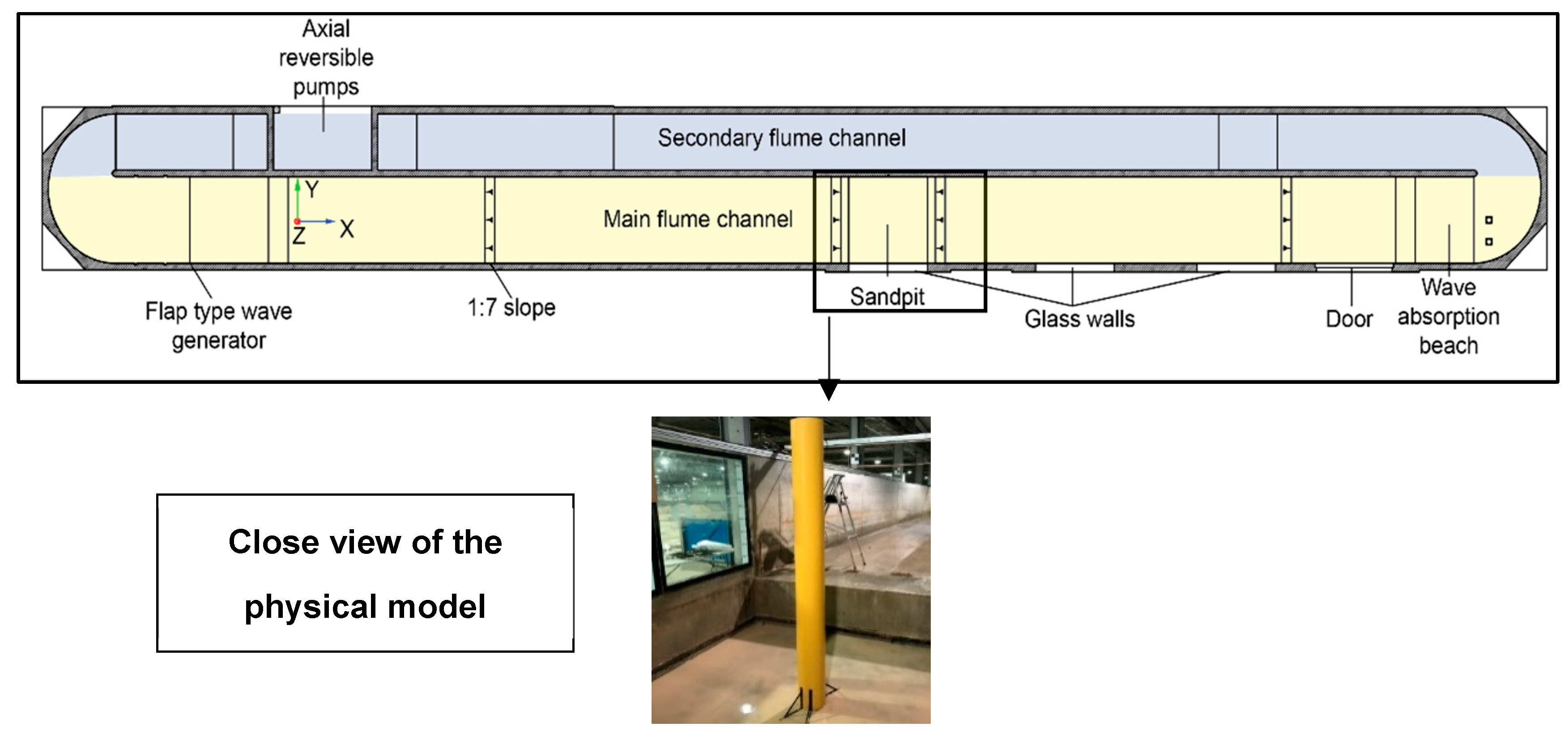
Funding

The work described in this publication was supported by the European Community’s Horizon 2020 Research and Innovation Program through the grant to HYDRALAB-PLUS, Contract no. 654110. The first author would like, in addition, to acknowledge his FWO (Research Foundation-Flanders, project number 3G052716) PhD. funding. Fazeres-Ferradosa was supported by the project POCI-01-0145-FEDER-032170 (ORACLE project), funded by the European Fund for Regional Development (FEDER), through the COMPETE2020, the Programa Operacional Competitividade e Internacionalização (POCI) and FCT/MCTES through national funds (PIDDAC).

Acknowledgments

The authors would like to thank HR Wallingford and the Ghent University technical teams for their availability and help throughout the testing campaign.

Conflicts of Interest

The authors declare no conflict of interest. This document reflects only the authors’ views and not those of the European Community. This work may rely on data from sources external to the HYDRALAB-PLUS project Consortium. Members of the Consortium do not accept liability for loss or damage suffered by any third party as a result of errors or inaccuracies in such data. The information in this document is provided “as is” and no guarantee or warranty is given that the information is fit for any particular purpose. The user thereof uses the information at its sole risk and neither the European Community nor any member of the HYDRALAB-PLUS Consortium is liable for any use that may be made of the information.

References

  1. Whitehouse, R.J.S. Scour at Marine Structures; Thomas Telford Ltd.: London, UK, 1998. [Google Scholar]
  2. Sumer, B.; Fredsøe, J. The Mechanics of Scour in the Marine Environment; Advanced series on ocean engineering; World Scientific: River Edge, NJ, USA, 2002. [Google Scholar]
  3. Chiew, Y.M. Mechanics of Riprap Failure at Bridge Piers. J. Hydraul. Eng. 1995, 121, 635–643. [Google Scholar] [CrossRef]
  4. Chiew, Y.; Lim, F. Failure behavior of riprap layer at bridge piers under live bed conditions. J. Hydraul. Eng. 2000, 126, 43–55. [Google Scholar] [CrossRef]
  5. Lauchlan, C.S.; Melville, B.W. Riprap protection at bridge piers. J. Hydraul. Eng. 2001, 127, 412–418. [Google Scholar] [CrossRef]
  6. Troch, P.; De Rouck, J.; Burcharth, H. Experimental study and numerical modeling of wave induced pore pressure attenuation inside a rubble mound breakwater. In Proceedings of the Coastal Engineering Conference, Cardiff, Wales, UK, 7–12 July 2002; pp. 1607–1619. [Google Scholar]
  7. Galay, V.J.; Yaremko, E.K.; Quazi, M.E. River Bed Scour and Construction of Stone Riprap Protection; Sediment Transport in gravel-bed rivers; Thorne, C.R., Bathurst, J.C., Hey, R.D., Eds.; John Wiley & Sons Inc.: New York, NY, USA, 1987; pp. 353–383. [Google Scholar]
  8. De Vos, L.; De Rouck, J.; Troch, P.; Frigaard, P. Empirical design of scour protections around monopile foundations. Part 2: Dynamic approach. Coast. Eng. 2012, 60, 286–298. [Google Scholar] [CrossRef]
  9. Loosveldt, N.; Vannieuwenhuyse, K. Experimental Validation of Empirical Design of a Scour Protection around Monopiles under Combined Wave and Current Loading. Master’s Thesis, Ghent University, Ghent, Belgium, 2012. [Google Scholar]
  10. Nielsen, A.W. Scour Protection of Offshore Wind Farms. Ph.D. Thesis, Technical University of Denmark, Lyngby, Denmark, 2011. [Google Scholar]
  11. Whitehouse, R.; Brown, A.; Audenaert, S.; Bolle, A.; de Schoesitter, P.; Haerens, P.; Baelus, L.; Troch, P.; das Neves, L.; Ferradosa, T.; Pinto, F. Optimising scour protection stability at offshore foundations. In Proceedings of the 7nd International Conference on Scour and Erosion (ICSE-7); CRC Press/Balkema, Leiden, The Netherlands, 2–4 December 2014; pp. 593–600. [Google Scholar]
  12. Petersen, T.U. Scour around Offshore Wind Turbine Foundations. Ph.D. Thesis, Technical University of Lyngby, Lyngby, Denmark, 2014. [Google Scholar]
  13. Schendel, A.; Goseberg, N.; Schlurmann, T. Experimental study on the performance of coarse grain materials as scour protection. Coast. Eng. Proc. 2014, 1, 58. [Google Scholar] [CrossRef]
  14. Schendel, A.; Goseberg, N.; Schlurmann, T. Erosion Stability of Wide-Graded Quarry-Stone Material under Unidirectional Current. J. Waterw. Port Coast. Ocean Eng. 2015, 142, 1–19. [Google Scholar] [CrossRef]
  15. CIRIA, CUR, CETMEF. The Rock Manual—The Use of Rock in Hydraulic Engineering, 2nd ed.; C683; CIRIA: London, UK, 2007; ISBN 978-0-86017-683-1. [Google Scholar]
  16. Petersen, T.U.; Nielsen, A.; Hansen, D.A.; Christensen, E.; Fredsoe, J. Stability of single-graded scour protection around a monopile in current. Scour and Erosion IX. In Proceedings of the 9th International Conference on Scour and Erosion (ICSE 2018), Taipei, Taiwan, 5–8 November 2018. [Google Scholar]
  17. Fazeres Ferradosa, T.; Taveira-Pinto, F.; Romão, X.; Vanem, E.; Reis, M.T.; Neves, L. Probabilistic design and reliability analysis of scour protections for offshore windfarms. Eng. Fail. Anal. 2018, 91, 291–305. [Google Scholar] [CrossRef]
  18. Sutherland, J.; Whitehouse, R.J.S. Scale Effects in the Physical Modelling of Seabed Scour; Technical Report TR 64; HR Wallingford Ltd.: Wallingford, Oxfordshire, UK, 1998. [Google Scholar]
  19. Hughes, S.A. Physical Models and Laboratory Techniques in Coastal Engineering; Advanced series on ocean engineering; World Scientific: River Edge, NJ, USA, 1993; Volume 7. [Google Scholar]
  20. Fazeres-Ferradosa, T.; Taveira-Pinto, F.; Reis, M.T.; das Neves, L. Physical modelling of dynamic scour protections: Analysis of the Damage Number. Proc. Inst. Civ. Eng. Marit. Eng. 2018, 171, 11–24. [Google Scholar] [CrossRef]
Figure 1. Sketch of the fast flow facility (FFF) flume channels including the position of the scale models.
Energies 12 01709 g001
Figure 2. Overview of the FFF main channel, and of the experimental setup including the intrumentation positions, the reference coordinate system and the scale model location.
Energies 12 01709 g002
Figure 3. (a) Monopile mounting base; (b) monopile scale model (scale 1:16) waiting to be installed; (c) monopile scale model placed on its support structure and external iron edges installed at the base.
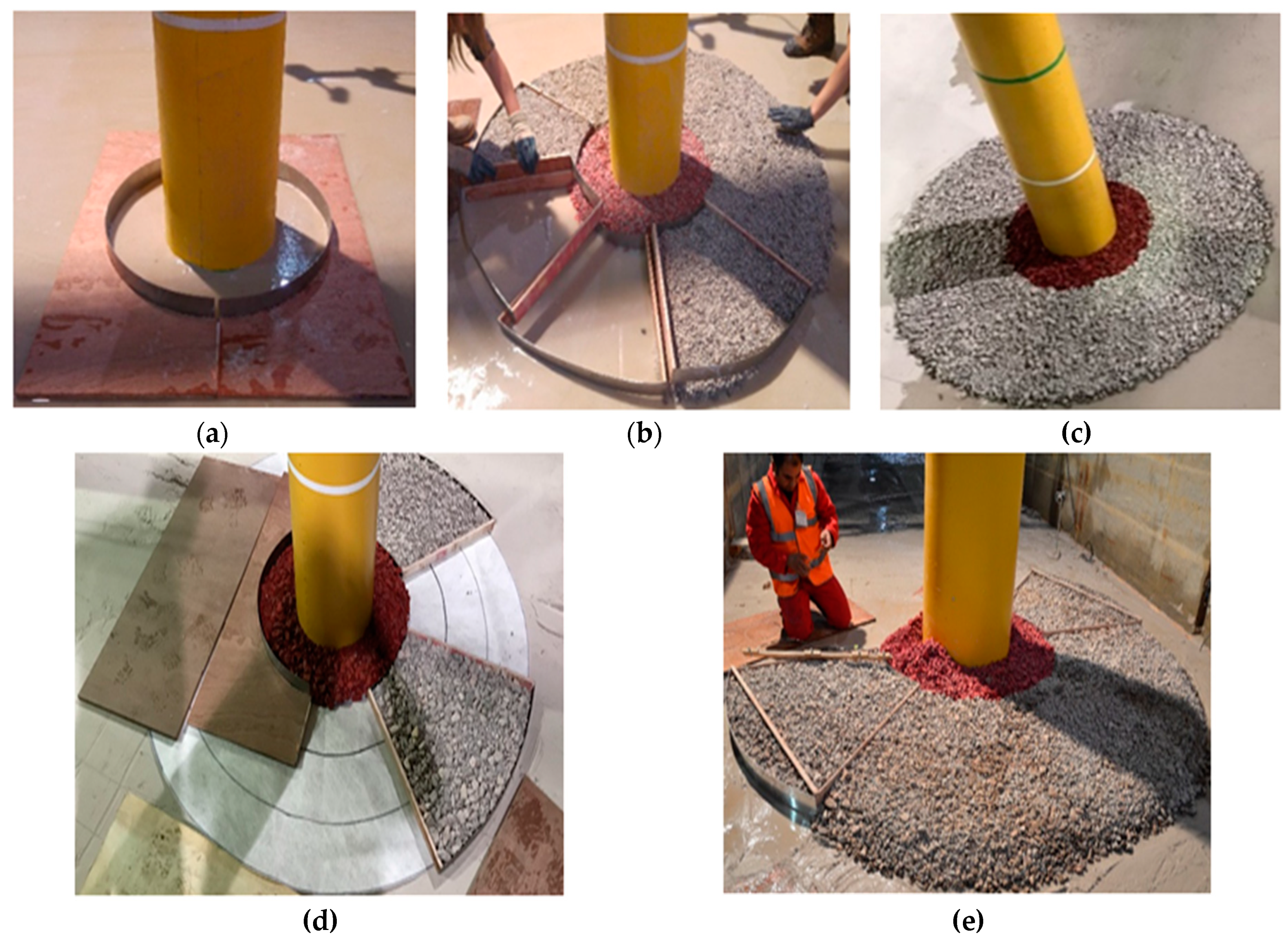
Energies 12 01709 g003
Figure 4. Installation of a scour protection scale model scale (scale 1:16.7). (a) Inner ring templates placed around the monopile; (b) outer ring placement using templates; (c) finalized scour protection model; (d) scour protection model placement over a geotextile; (e) placement of a scale model (scale 1:8.3) using larger templates.
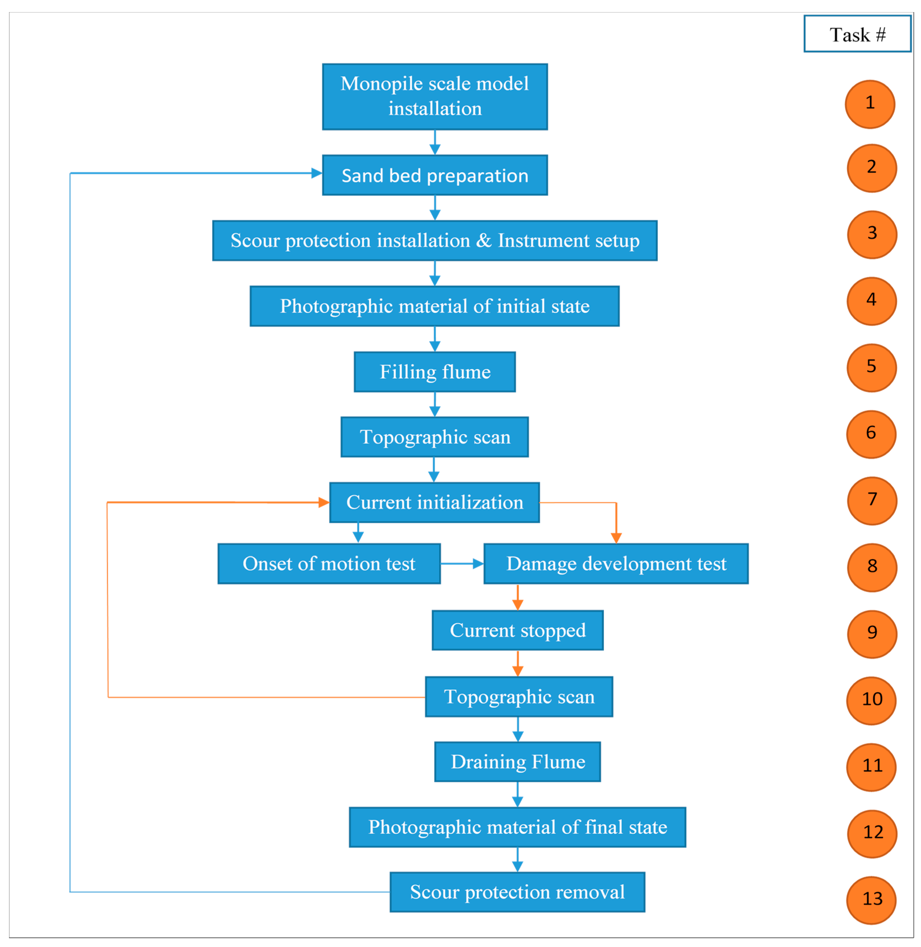
Energies 12 01709 g004
Figure 5. Flow chart of experiment execution. The loop indicated using orange arrows is performed three times for Test No. 14 and twice for the other damage development tests.
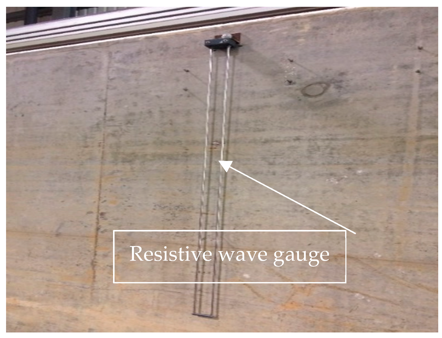
Energies 12 01709 g005
Figure 6. Example of resistive wave gauge used during the Protection of offshore wind turbine monopiles against scouring (PROTEUS) project.
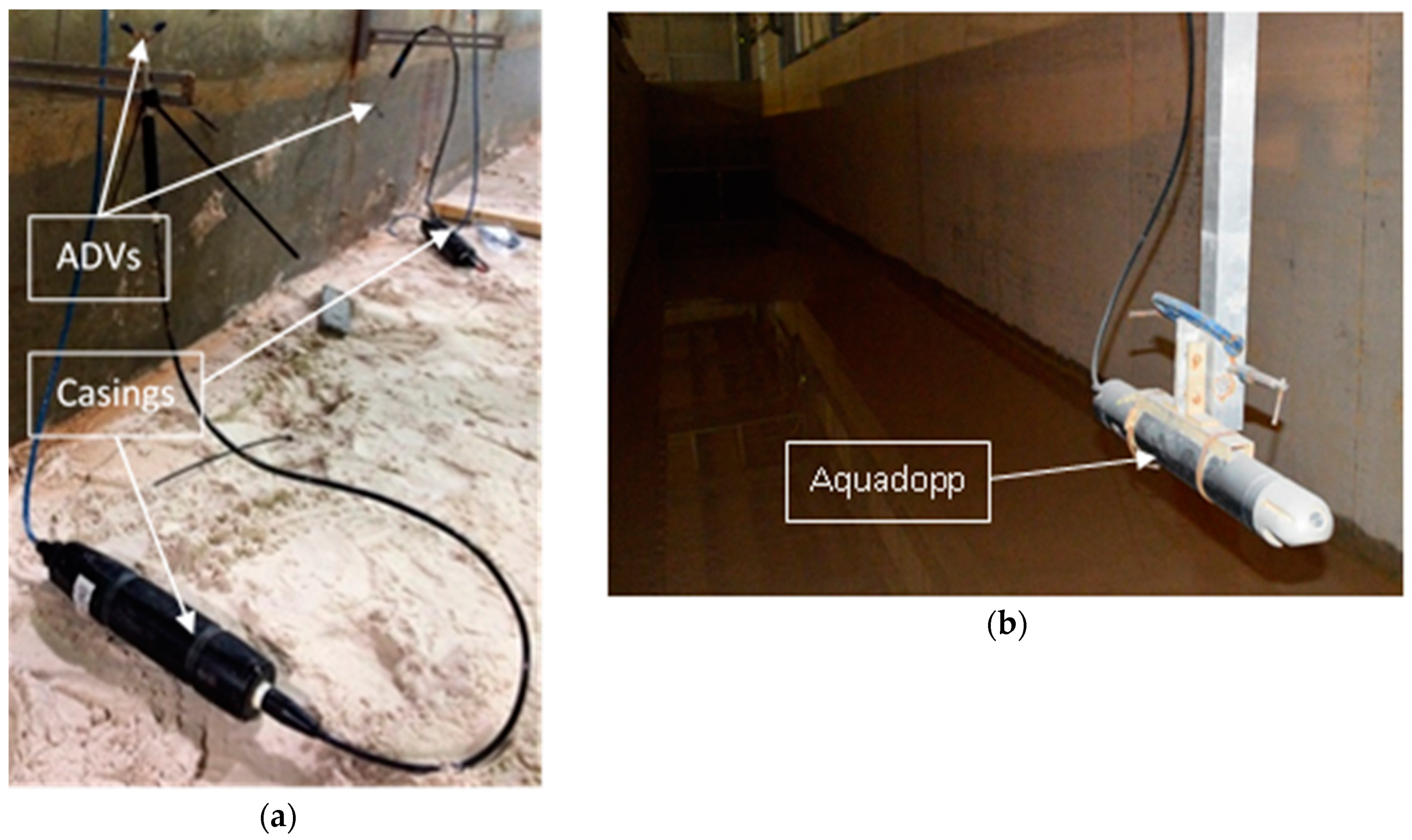
Energies 12 01709 g006
Figure 7. Instrumentation used for velocity measurements: (a) two ADVs placed above the sand pit; (b) down-facing Aquadopp profiler placed in the secondary flume channel. The Aquadopp vertical position was z = −0.83 m for water depths 0.9 m and 1.2 m and z = −0.91 m for water depths 1.5 m and 1.8 m.
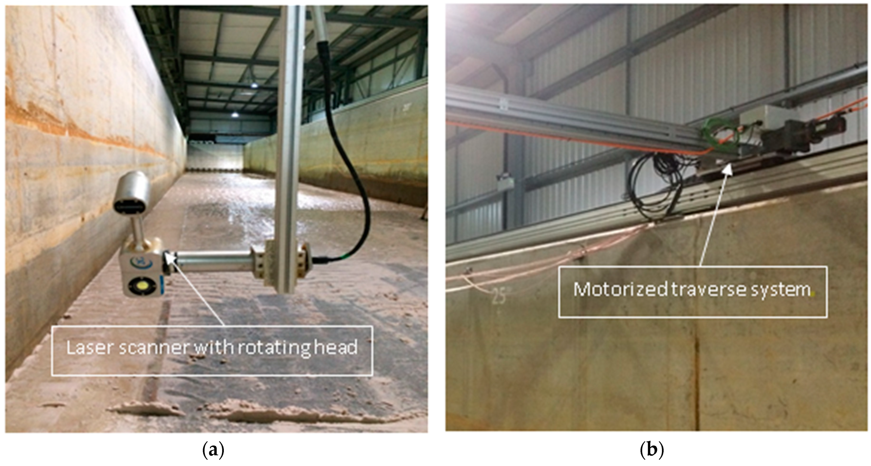
Energies 12 01709 g007
Figure 8. (a) The ULS-200 laser scanner with rotating head. (b) The motorized transverse system.
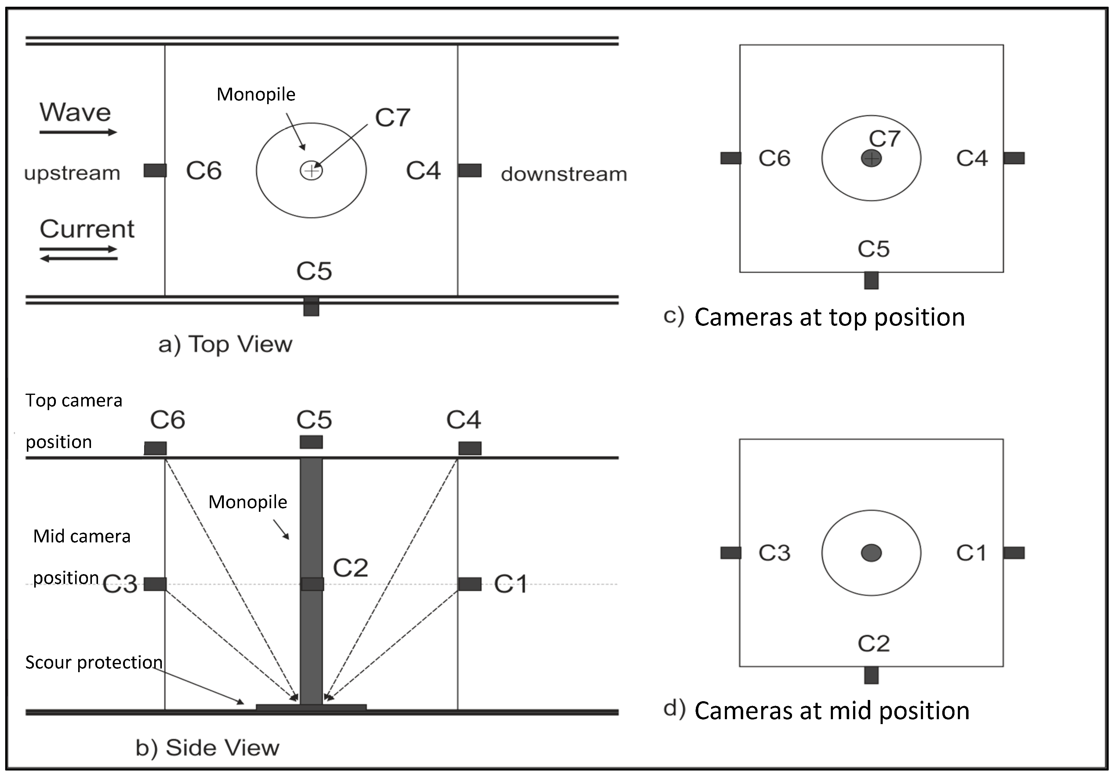
Energies 12 01709 g008
Figure 9. Camera position for photographic material recording.
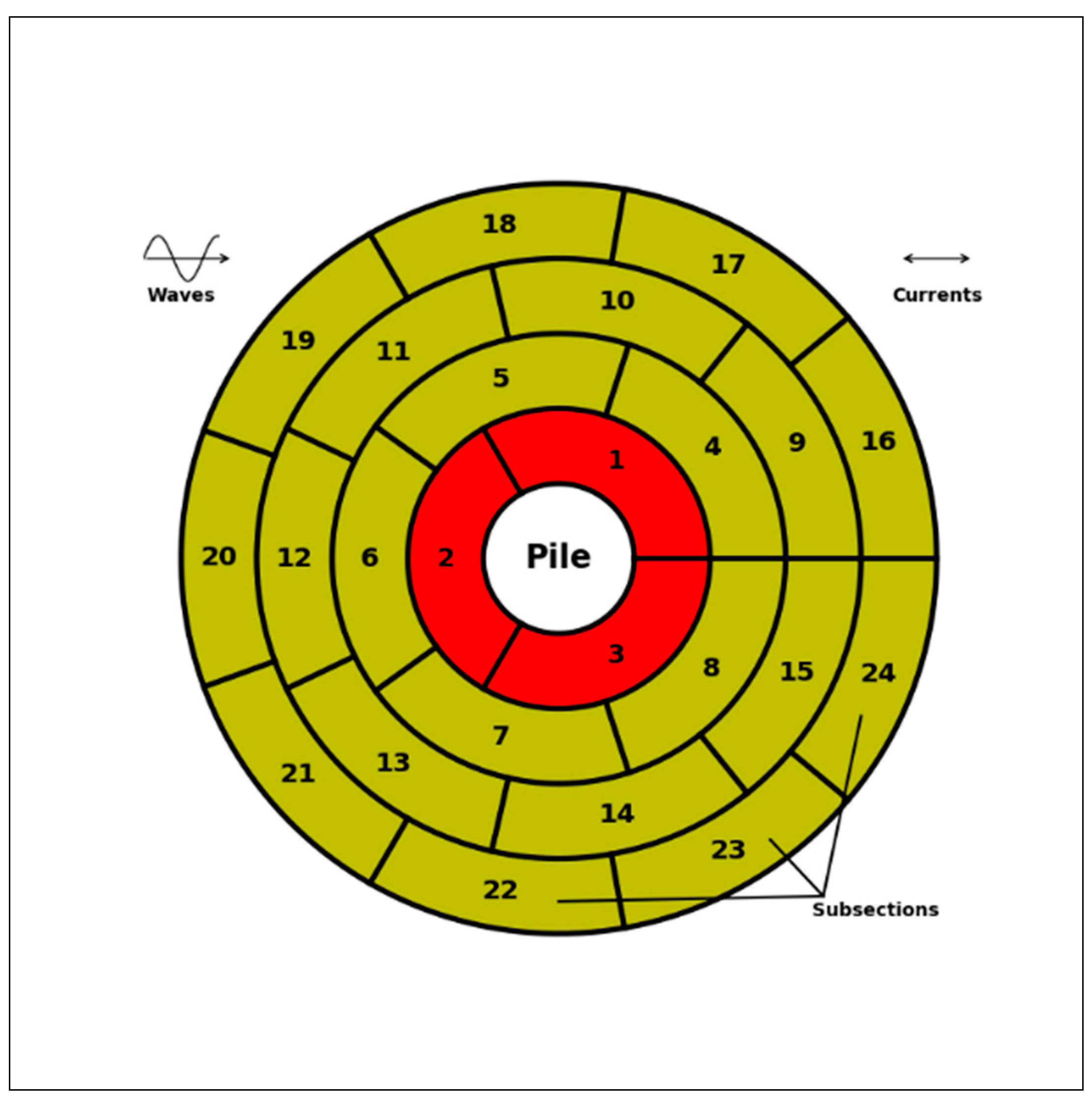
Energies 12 01709 g009
Figure 10. Sketch of the scour protection model around the monopile divided in subsections as in [8], with the inner ring in red. The waves and current propagation directions are also indicated. The decomposition in subsections is made depending on the direction of propagation of the current. The present setup is for a current propagation opposing waves, the setup should be mirrored if the current follows the waves.
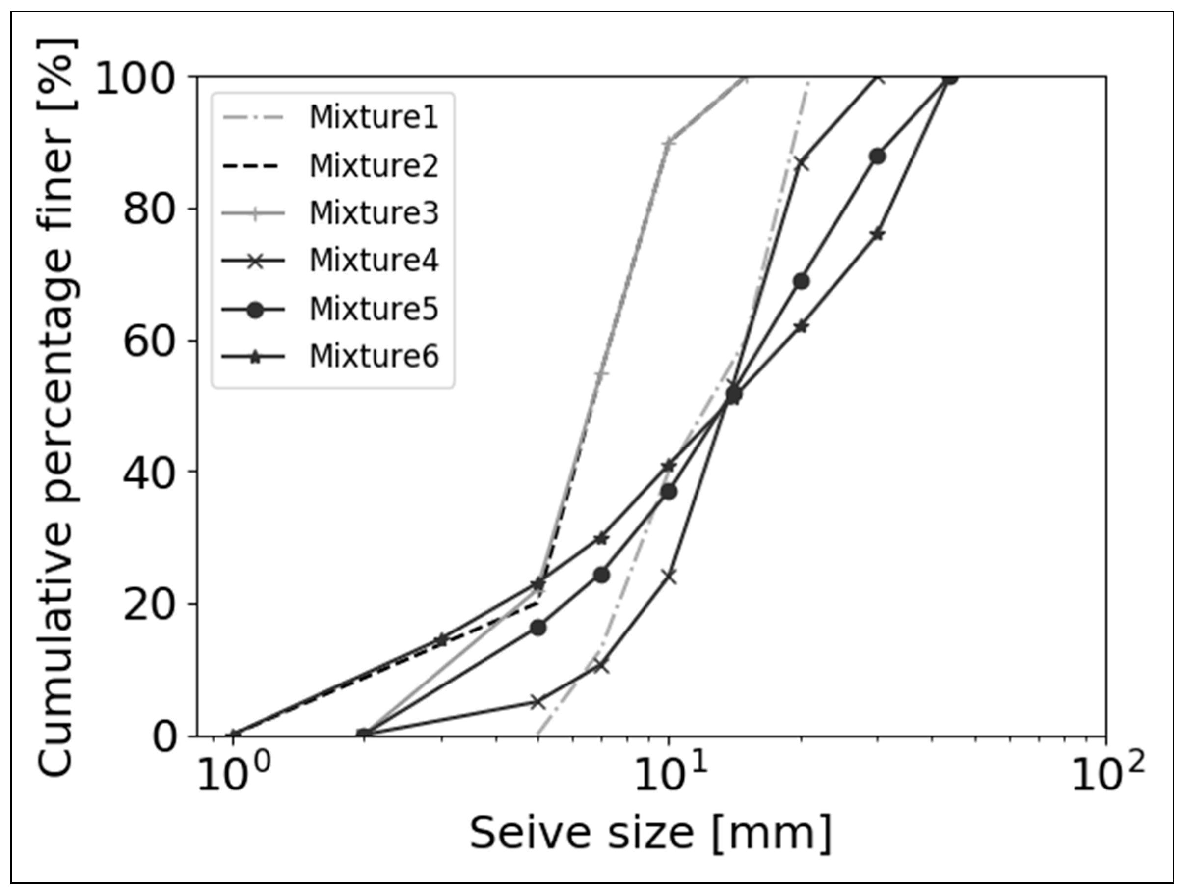
Energies 12 01709 g010
Figure 11. Percentage finer against the sieve size for the 6 tested mixtures.
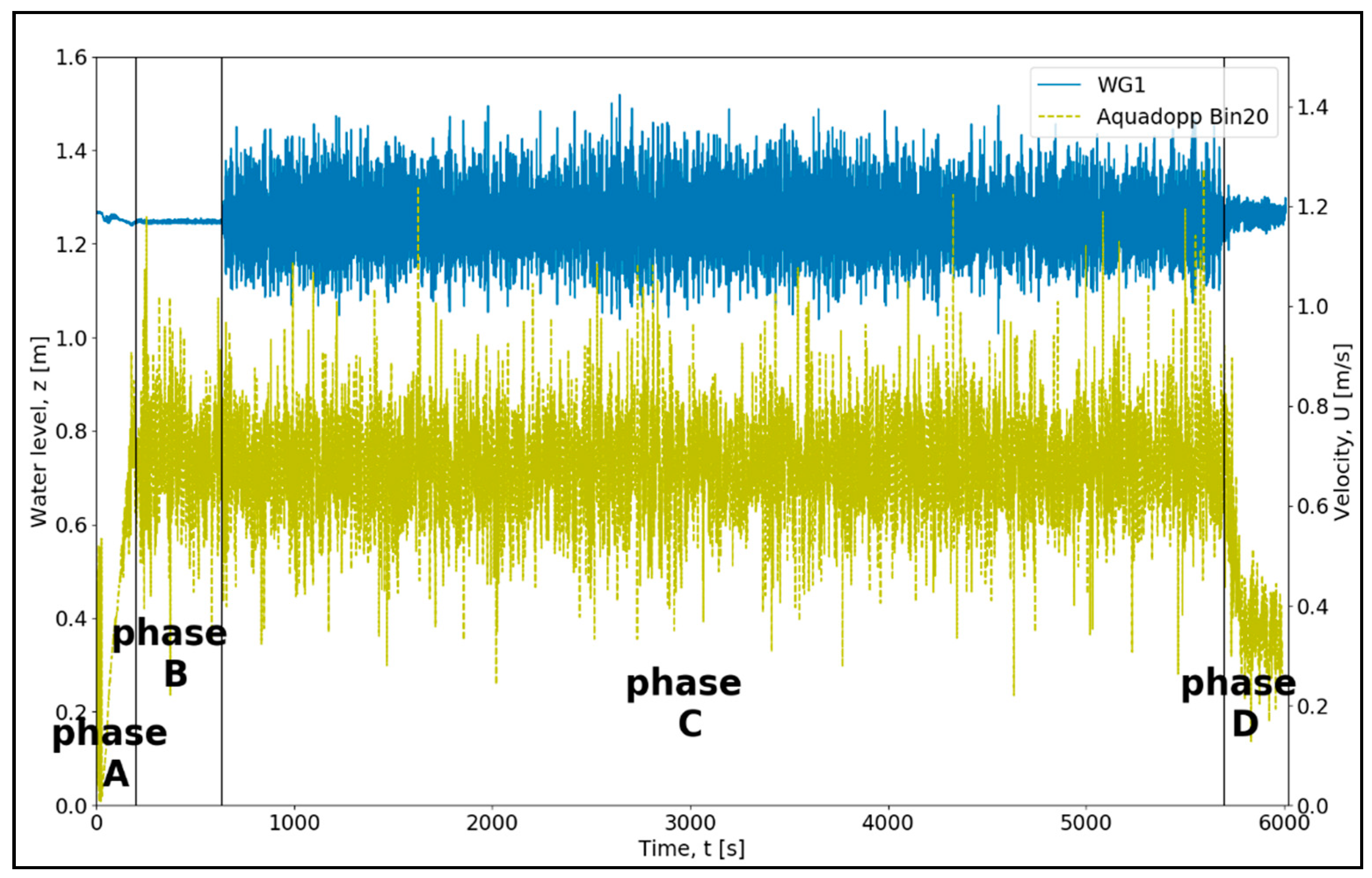
Energies 12 01709 g011
Figure 12. Test 04_B measurement of WG1 (left vertical axis) and Aquadopp at bin 20 (right vertical axis) with test phases: (“phase A”) Initialization of the test (time: 0–200 s); (“phase B”) Current stabilization (time: 200–633 s); (“phase C”) Wave Generation (time: 633–5697 s); (“phase D”) Test finalization and water level stabilization (time: 5691–6010 s).
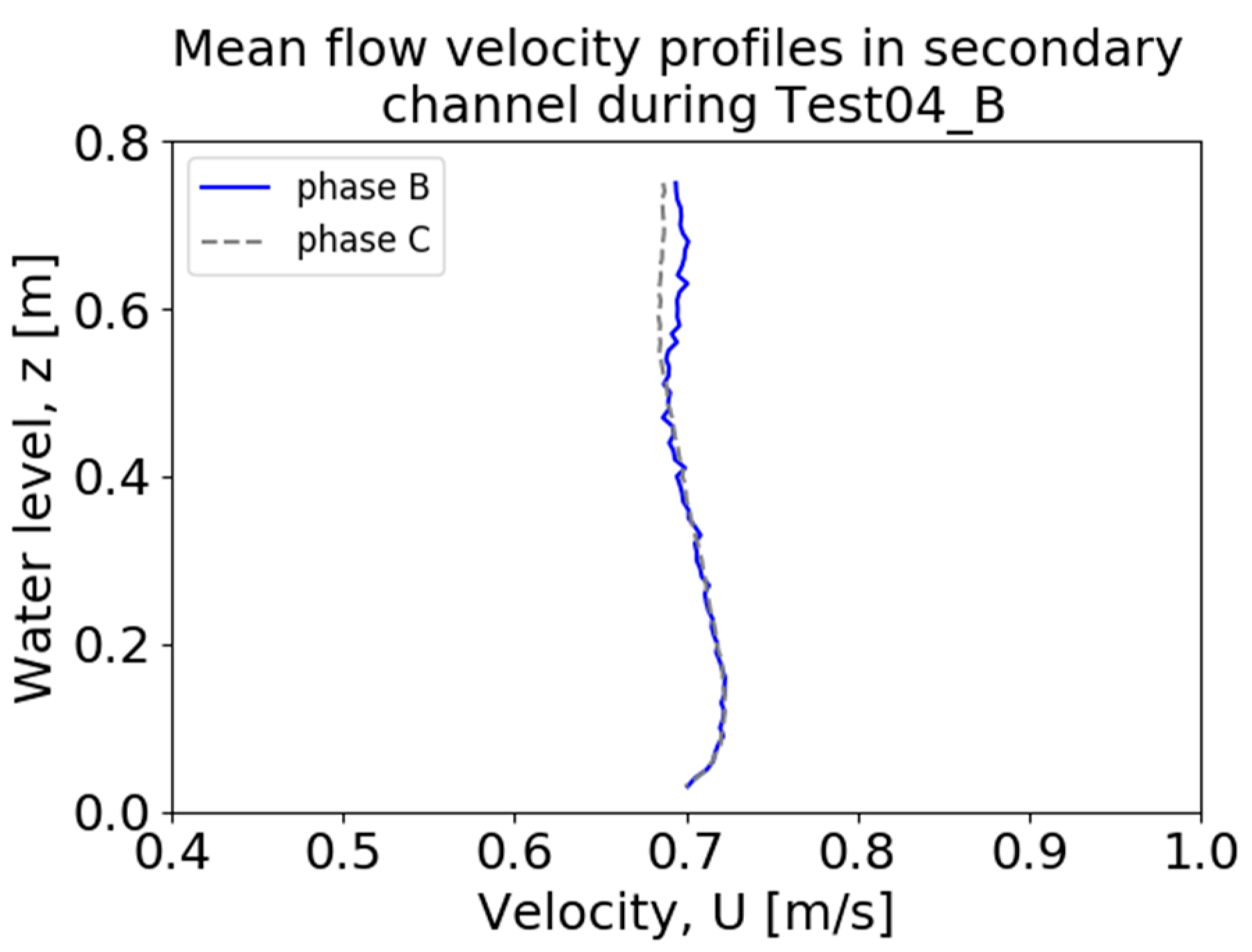
Energies 12 01709 g012
Figure 13. Mean profile velocity from Aquadopp measurements during current stabilization (phase B) and wave generation phase (phase C) of Test 04_B over the water column.
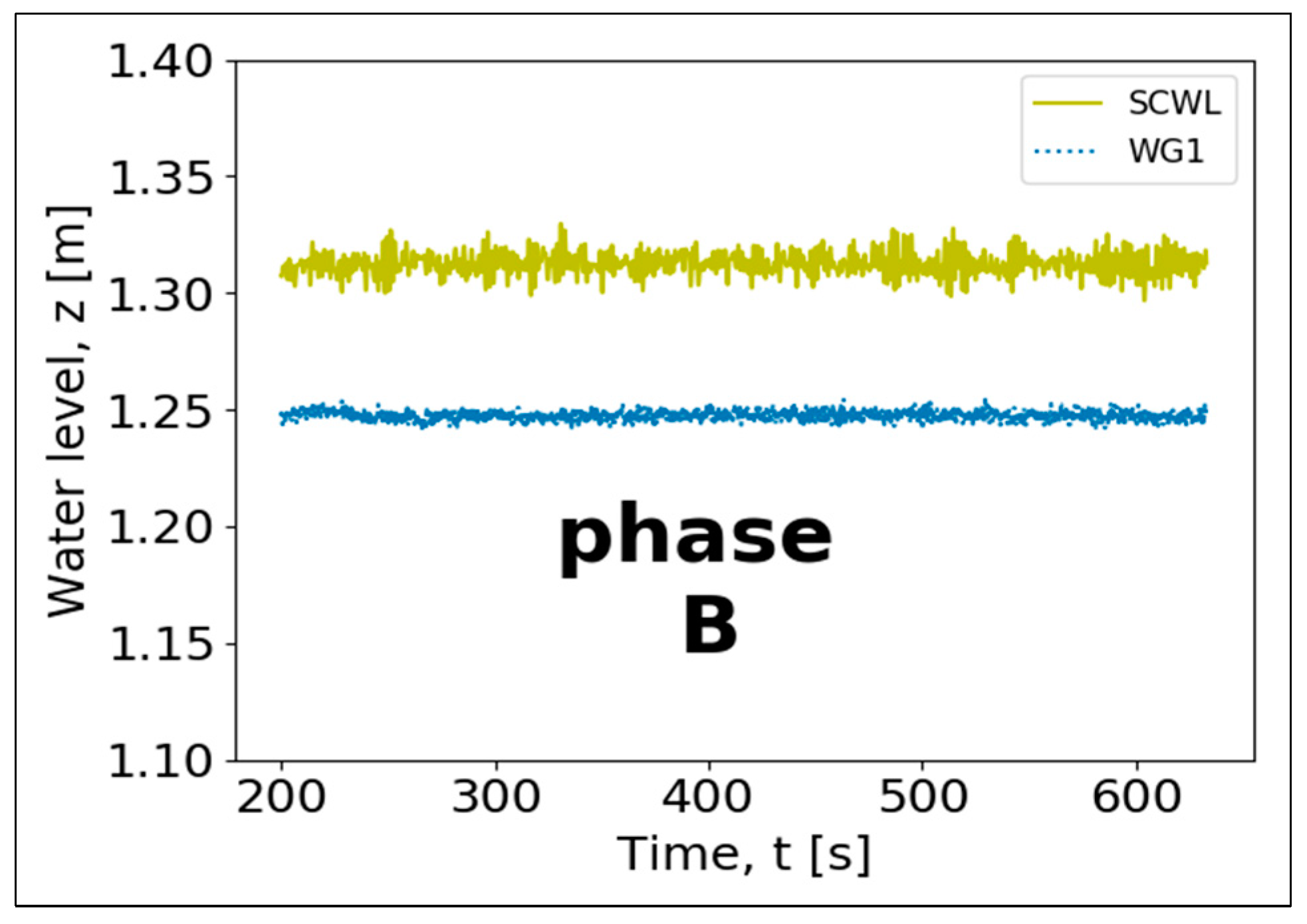
Energies 12 01709 g013
Figure 14. Secondary channel water level (SCWL) and WG1 measurements during the current stabilization phase B of Test 04_B.
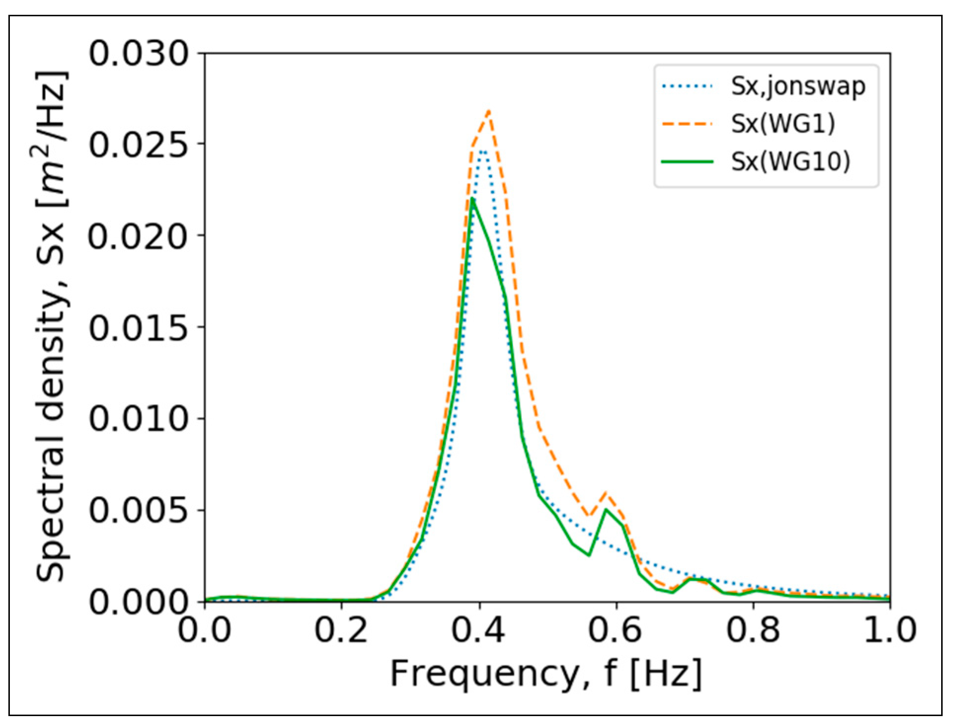
Energies 12 01709 g014
Figure 15. Spectral density of the target JONSWAP spectrum, Sx, jonswap, and free surface measurements of WG1, Sx(WG1), and WG10, Sx(WG10), for test 04_B over the frequency, f.
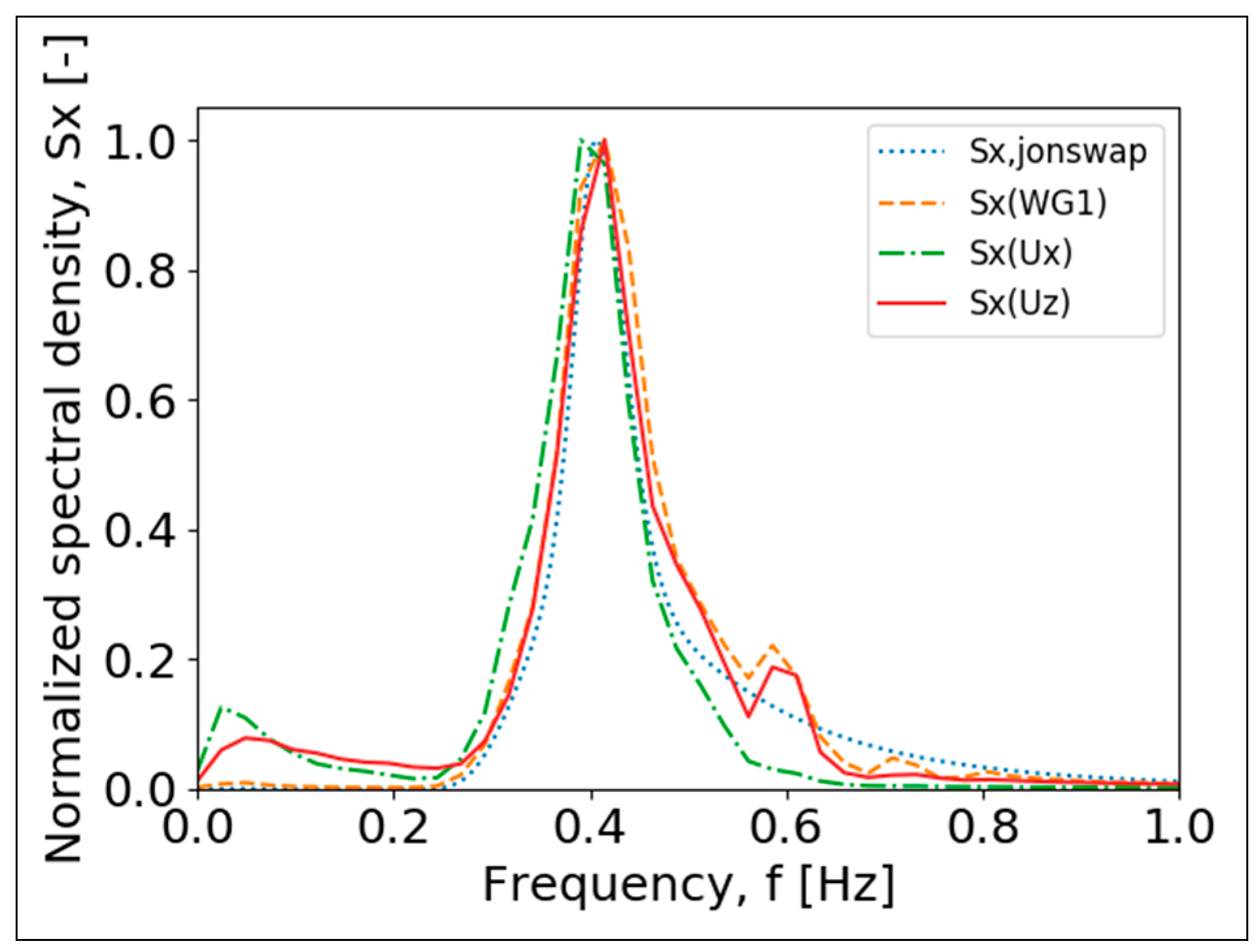
Energies 12 01709 g015
Figure 16. Normalized spectral density of target JONSWAP, Sx, jonswap, measurements of water level, Sx(WG1), and ADV velocity measurements (ADV2) x-components, Sx(Ux), and z-components, Sx(Uz), over the frequency.
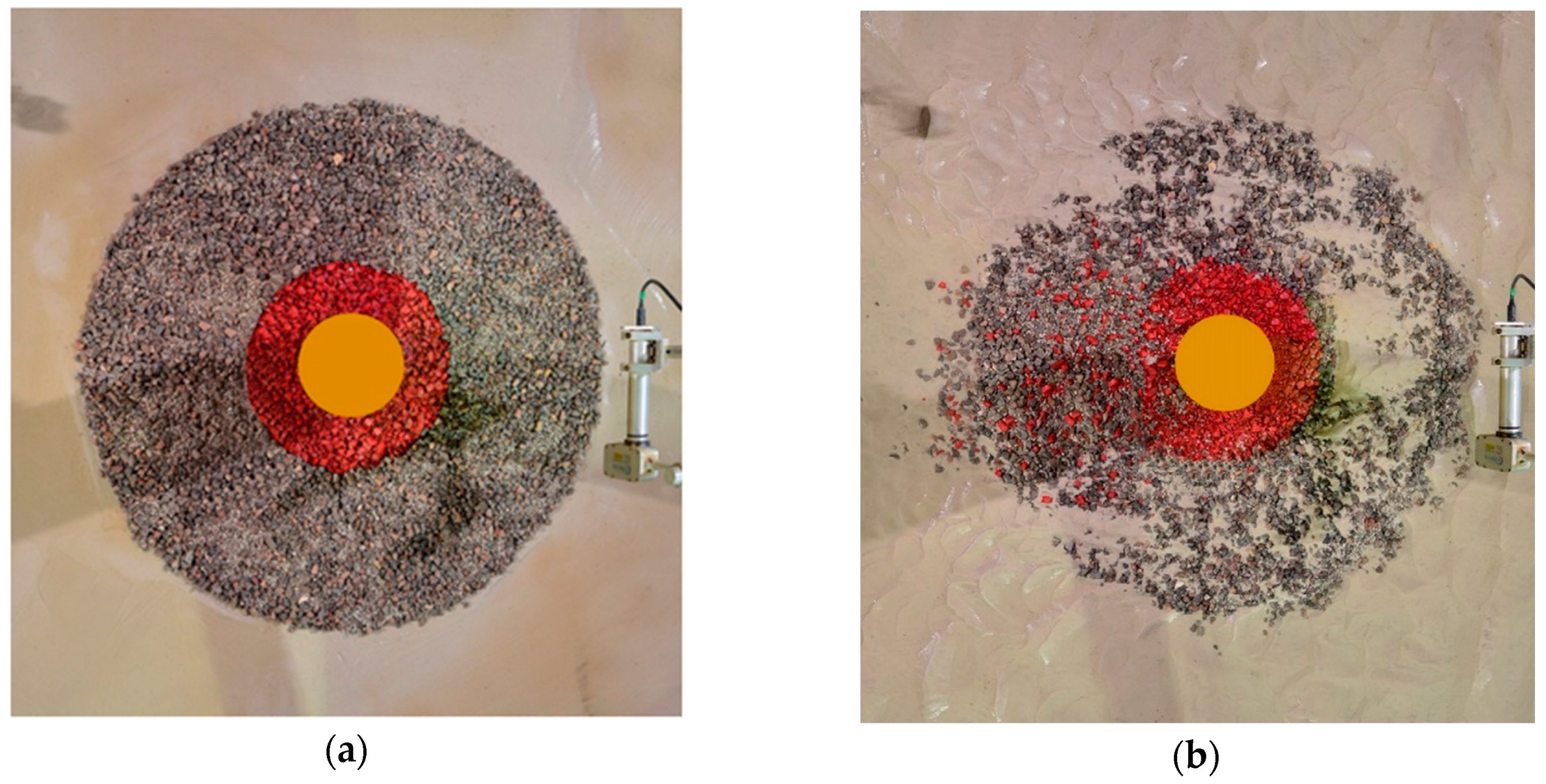
Energies 12 01709 g016
Figure 17. Merged picture of the scour protection scale model Tests 04 before (a) and after (b) the test. The current propagation in this set of figures is from right to left.
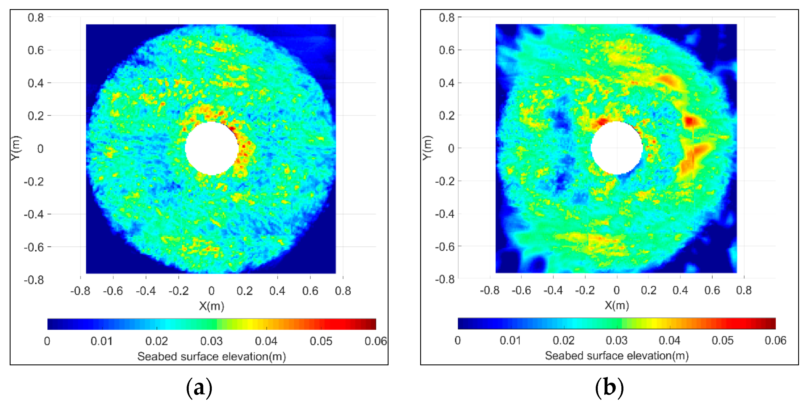
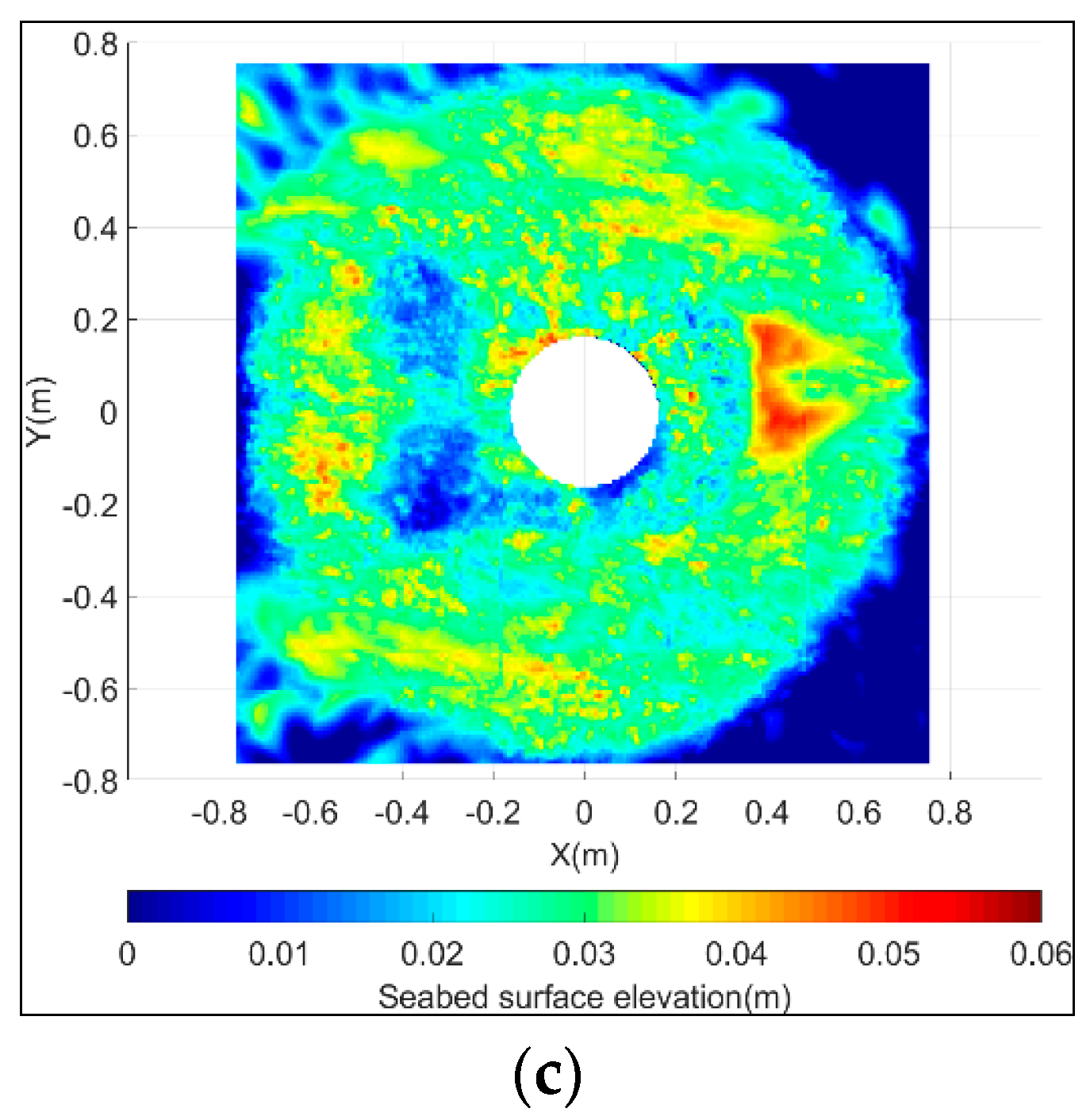
Energies 12 01709 g017
Figure 18. Topography of the scour protection material and of the sand pit measured by the laser scanner before Test 03 (a), after the first 1000 waves of Test 04_A (b) and after 3000 waves at the end of Test 04_B (c). The current propagation in this set of figures is from right to left.
Energies 12 01709 g018aEnergies 12 01709 g018b
Figure 19. Test 04 subdivision damage number: after 1000 waves Test 04_A (a) and after 3000 waves Test 04_B (b). The current propagation in this set of figures is from right to left.
Energies 12 01709 g019
Table 1. Measured parameters and instrumentation.
Measured ParameterInstrumentation
Free surface elevationResistive wave gauges (WGs)
Flow velocities3D point measurementsAcoustic doppler velocity meters (ADVs)
Profile measurements of the horizontal velocityAquadopp profiler
Scour protection model topographyULS-200 laser scanner
Photographic materialCameras
Table 2. Positions of the wave gauges following the local coordinate system indicated in Figure 1 and Figure 2.
Wave Gauge No.Position in x-Direction (m)Position in y-Direction (m)
WG122.591.97
WG223.491.97
WG324.481.97
WG426.001.97
WG530.241.97
WG630.19−1.95
WG734.601.97
WG835.501.97
WG936.531.97
WG1038.911.97
Table 3. Positions of the Aquadopp profiler and the two ADVs following the local reference system, as indicated in Figure 1 and Figure 2.
InstrumentPosition in x-Direction (m)Position in y-Direction (m)Position in z-Direction (m)
Aquadopp29.50 (middle of secondary flume)−0.86
ADV130.301.70−0.4d
ADV231.601.70−0.4d
Table 4. Onset of motion measured test conditions. The highlighted conditions are the ones where the motion of scour protection material is spotted. S/N stands for the serial number.
Test No.Water DepthMonopile DiameterCurrent VelocityTest VariantWave HeightWave Period
S/Nd (m) D p (m) U c (m/s)S/NH (m)T (s)
031.20.3−0.25A0.222.94
B0.282.94
C0.272.94
D0.332.47
E0.392.47
051.50.30.27A0.202.91
B0.222.93
C0.282.98
D0.322.94
E0.352.94
F0.322.51
G0.372.48
071.20.3−0.23A0.252.94
B0.292.94
C0.332.46
D0.312.46
090.90.3−0.23A0.202.46
B0.222.06
C0.262.08
111.80.6−0.39A0.503.50
B0.373.48
C0.423.48
D0.543.48
E0.412.84
F0.462.85
G0.502.83
H0.562.85
The onset of motion tests with clear motion of the scour protection material are highlighted.
Table 5. Damage development measured conditions.
Test No.VariantSignificant Wave HeightPeak Wave PeriodMain Channel Computed Average Flow VelocityMean Flow Velocity Secondary ChannelMean Flow Velocity ADV1Mean Flow Velocity ADV2Number of Waves
S/NS/N H s (m) T p (s) U c o m p (m/s) U S C (m/s) U A D V 1 (m/s) U A D V 2 (m/s)N (-)
04A0.252.45−0.49−0.70−0.46−0.461000
B0.242.48−0.50−0.70−0.46−0.462000
06A0.282.20−0.380.620.390.381000
B0.282.20−0.37−0.590.390.382000
08A0.192.44−0.50−0.70−0.46−0.451000
B0.192.44−0.50−0.70−0.46−0.452000
10A0.182.05−0.33−0.46−0.30−0.281000
B0.162.05−0.33−0.46−0.30−0.292000
12A0.372.81−0.50−0.75−0.51-1000
B0.382.83−0.51−0.75−0.52-2000
13A0.332.34−0.57−0.83−0.63-1000
B0.342.35−0.57−0.83−0.63-2000
14A0.392.83−0.51−0.75−0.49-1000
B0.412.83−0.51−0.75−0.49-2000
C0.412.90−0.51−0.76−0.49-2000
15A0.412.88−0.49−0.74--1000
B0.392.86--−0.49-2000
Table 6. Properties of scour protection composition and indication of usage.
Scour Protection Mixture No.Test No.Mean DiameterGradation of the Material
S/NS/N D 50 (mm) D 85 / D 15 (-)
103/0412.52.48
205/066.752.48
307/08/09/106.752.48
411/12/1313.52.48
51413.56
61513.512
7 (Geotextile)03/04/07/08--
Table 7. Average main channel water level (MCWL), secondary channel water level (SCWL) and WG water level measurements for test 04_B.
Avg. SCWL (m)WG1 (m)WG2 (m)WG3 (m)WG4 (m)WG5 (m)WG6 (m)WG7 (m)WG8 (m)WG9 (m)WG10 (m)Avg. MCWL (m)
1.3121.2471.2441.2441.2461.2471.2461.2481.2481.2461.251.247
Table 8. Average velocity of the flow in the main and secondary channel acquired by different methods and the computed velocity of the flow for Test 04_B in phase B.
Mean Flow Velocity ADV1Mean Flow Velocity ADV2Mean Flow Velocity Secondary ChannelMain Channel Computed Average Flow Velocity
U A D V 1 (m/s) U A D V 2 (m/s) U S C (m/s) U c o m p (m/s)
0.460.460.700.50
Table 9. Wave characteristics from spectral analysis of the WGs measurements and mean values for Test 04_B.
ParameterSignificant Wave HeightPeak PeriodWave Energy PeriodFirst Moment Wave PeriodMean Zero Up-Crossing Period
Symbol H m 0 T p T m 1 , 0 ( T e ) T m 0 , 1 T m 0 , 2 ( T z )
Unit(m)(s)(s)(s)(s)
Target value0.2252.46---
WG10.2552.402.492.212.04
WG20.2582.402.502.191.83
WG30.2572.562.502.181.77
WG40.2492.402.502.211.89
WG50.2262.402.532.242.08
WG60.2732.402.472.211.91
WG70.2152.562.542.252.03
WG80.2192.562.522.221.79
WG90.2222.562.512.221.79
WG100.2222.562.572.2491.98
Mean value0.2402.482.512.221.91
Table 10. Measured and predicted S3D number for Test 04_A and 4_B.
Test No.Mean Grain SizeGradationNumber of WavesPile DiameterWater DepthSignificant Wave HeightPeak PeriodHorizontal Wave Orbital VelocityMean Current VelocityPredicted Damage NumberMeasured Damage Number
D 50 (mm) D 85 / D 15 (-)N (-)Dp (m)d (m)Hs (m)Tp (m)Um (m/s)Uc (m/s)Predicted S3DMeasured S3D
Test 04_A12.52.4810000.31.20.252.450.177−0.461.8340.465
Test 04_B12.52.4820000.31.20.242.480.166−0.462.1410.675

