Low-Level Control of Hybrid Hydromechanical Transmissions for Heavy Mobile Working Machines

Abstract

Fuel efficiency has become an increasingly important property of heavy mobile working machines. As a result, Hybrid Hydromechanical Transmissions (HMTs) are often considered for the propulsion of these vehicles. The introduction of hybrid HMTs does, however, come with a number of control-related challenges. To date, a great focus in the literature has been on high-level control aspects, concerning optimal utilization of the energy storage medium. In contrast, the main topic of this article is low-level control, with the focus on dynamic response and the ability to realize requested power flows accurately. A static decoupled Multiple-Input-Multiple-Output (MIMO) control strategy, based on a linear model of a general hybrid HMT, is proposed. The strategy is compared to a baseline approach in Hardware-In-the-Loop (HWIL) simulations of a reference wheel loader for two drive cycles. It was found that an important benefit of the decoupled control approach is that the static error caused by the system’s cross-couplings is minimized without introducing integrating elements. This feature, combined with the strategy’s general nature, motivates its use for multiple-mode transmissions in which the transmission configuration changes between the modes.

1. Introduction

Environmental concerns, stricter legislation, and demands for higher productivity have increased the interest in hydraulic hybrid transmissions for heavy mobile working machines. For these vehicles, the combination of an Internal Combustion Engine (ICE) with hydraulic accumulators offers attractive improvements on several points, such as energy efficiency, productivity, and machine operability [1]. Hydraulic hybridization does, however, tend to increase the reliance on control. In this context, a commonly-addressed challenge concerns the optimal use of the added power source; continuously during vehicle operation, a proper decision is required whether the accumulator should be charged or discharged [2]. The maker of this decision is commonly referred to as a high-level control strategy and has been investigated for both on-road vehicles [3,4] and mobile working machines in the past [5,6,7].

Regardless of the performance of the high-level control, a hydraulic hybrid working machine relies on a stable, accurate, and properly-implemented low-level control. This aspect has been addressed limitedly for this application in the past and is the primary focus of this paper. An approach based on decoupled Multiple Input Multiple Output (MIMO) control, previously derived by the authors [8], is presented and compared to a baseline approach in two drive-cycles for a reference vehicle in Hardware-In-the-Loop (HWIL) simulations. For decoupling, the approach uses a linear model of a general hybrid multiple-mode Hydromechanical Transmission (HMT) suited for the characteristic features of a heavy mobile working machine, in this paper exemplified as a wheel loader.

In this paper, the low-level control refers to the concept applied in traditional control theory, for which the focus is on system response, dynamics and stability, rather than fuel efficiency. Its purpose is thus to handle the realization and dynamic coordination of the power flows demanded by the machine operator and the high-level control strategy [2].

1.1. Previous Work

A fundamental principle within low-level control of hydraulic hybrids is secondary control, which has been present in fluid power research since the 1980s; see, e.g., [9,10]. In this concept, the idea is that speed control takes place directly at the load. In the rotating domain, this idea is enabled by subjecting a variable displacement pump/motor (unit) to a constant pressure. This way, the unit’s shaft torque is proportional to its displacement setting, which in turn, may be used for closed loop control of the shaft speed. Consequently, the stability and response of secondary controlled systems rely on fast and accurate displacement controllers [11,12].

Secondary control is central in the control of hydraulic hybrids as it enables energy recuperation; when braking a load, the unit may work as a pump to charge an accumulator. Some aspects, however, distinguish the low-level control of hydraulic hybrid vehicles from pure secondary control. First, the secondary control loop in a vehicle is the operator who varies the output torque to control the vehicle speed, a concept commonly referred to as torque control [13]. Second, the system pressure is not constant, but impressed [11], due to the accumulator’s high capacitance. This means that the system pressure does vary, but slowly, with the accumulator’s state-of-charge. The state-of-charge is controlled by the high-level strategy, and pressure control is consequently required of the low-level controllers. Third, a hybrid vehicle contains an ICE, which requires active speed control to ensure maximum efficiency operation. The propriety of how these aspects are handled depends, in turn, on the considered hybrid configuration and what is feasible in the specific application. Various solutions are therefore found in the literature.

For on-road vehicles, an early example is the Cumulo series hydraulic hybrid system for city buses [14]. In these systems, output torque control was handled by the secondary unit, while engine speed was controlled by the primary unit. The engine control was limited to an internal droop governor, which was used for pressure control based on a vehicle speed-dependent high-level strategy. In more recent research, power-split hybrids are often considered for high efficiency, and usually, the engine control loop is considered more flexible and available for detailed control design. One aspect that arises with power-split hybrids is that different configurations facilitate torque control to different degrees [13]. The Output-Coupled-Power-Split (OCPS) hydraulic hybrid configuration has been studied by Kumar et al. [15], in which one hydraulic unit was used for torque control and the other for pressure control. For the ICE, sliding mode control with rejection of torque disturbances from the transmission was proposed. In [3,16], a hierarchical control strategy for power-split hybrids was proposed. In this case, both hydraulic units handle the torque control, while one unit indirectly manages the pressure control by loading the engine with an optimal torque demanded by a mid-level strategy. A PI-controller with feedforward of the transmission torques for disturbance rejection was used for engine speed control.

In contrast to the research presented above, this paper focuses on heavy mobile working machines. These are different from on-road applications on several points, which has an effect on the low-level control. Here, the wheel loader is used as an example, but the reasoning is valid for many other working machines as well.

1.2. Wheel Loaders

Wheel loaders are very versatile working machines. Compared to on-road vehicles, they typically operate in short, repetitive cycles with high power transients. In addition to the driveline, wheel loaders also have work functions, thereby resulting in multiple substantial power consumers. These aspects have a strong influence on both the design [7] and high-level control [5] of hybrid wheel loaders and should consequently also be taken into account in the low-level control. In addition, the unique conditions and complex nature of wheel loaders make the operator play a key role in maximizing their performance [17]. In this sense, torque control of the transmission is usually desired and expected by the operator [18].

Compared to on-road vehicles, large wheel loaders require wider speed/torque conversion ranges of the transmission. As a result, power-split non-hybrid HMTs are often seen as viable alternatives to the hydrodynamic (torque-converter) transmission [19]. These systems combine a Hydrostatic Transmission (HST) with planetary gear trains, thereby enabling high efficiency and optimal engine operation [20]. Usually, multiple-mode HMTs with clutches are required for sufficient conversion range, efficiency, and power density [21]. Each mode then consists of one of the commonly-mentioned single-mode configurations; Input-Coupled Power-Split (ICPS), Output-Coupled-Power-Split (OCPS), and compound [22].

A hybrid HMT is, in this paper, referred to as an HMT with a hydraulic accumulator in the HST circuit, and the term thereby covers both series and power-split hybrid configurations. The commonly-mentioned parallel hybrid is out of scope of this paper. See [1] for an attempt to map all hybrid configurations possible for both driveline and work functions of a wheel loader.

1.3. Summary: Demands on the Low-Level Control for Mobile Working Machines

In light of the topics discussed in the previous sections, the low-level control strategy for the transmission of a heavy hydraulic hybrid mobile working machine may be expected to:

• be easy to connect to a high-level control strategy,
• take displacement controller dynamics into account,
• handle pressure control,
• handle ICE speed control,
• ensure that torque control for the operator is achieved,
• take disturbances from external loads and additional power consumers into account,
• be easy to apply to a multiple-mode power-split transmission configuration.

In this paper, decoupled MIMO control is considered as a suitable candidate for this strategy.

1.4. Decoupled Control

The basic idea of decoupled control is that a MIMO system is converted into a number of Single-Input-Single-Output (SISO) loops that are treated as individual systems. This is done by first implementing a suitable decoupling strategy, usually based on a model of the system in question [23]. Hybrid HMTs contain system cross-couplings [8], and decoupled control may handle these with simple implementation and tuning [24]. Another aspect that motivates decoupled control of hybrid HMTs is that one of the controllers is the driver who controls the output speed. This loop is, therefore, out of reach for the control design and should then be as decoupled as possible. In addition, the decoupled strategy may be used to translate the system to one that is independent of the transmission configuration. This feature is highly attractive in a multiple-mode concept, since the configuration changes in between each mode, and the mode shift should be as smooth as possible [25].

1.5. Objective and Delimitations

The main objective of this paper is to present experimental results showing the principal-of-operation of a proposed decoupled control strategy. This is carried out in HWIL simulations of a reference vehicle for two cases. The first is a simplified load-and-carry drive cycle, and the second is a series of step responses. The proposed strategy is compared to a baseline approach, which ignores the system’s cross-couplings. The purpose of this comparison is to evaluate the couplings’ effect on control performance and how this effect is handled by the decoupled strategy.

The analysis is limited to the control within a single mode, i.e., mode shifts are not considered, and the reference transmission is of the single-mode type. Furthermore, the primary focus is on the transmission, and work functions are considered as disturbance torques or flows.

2. Linear Model

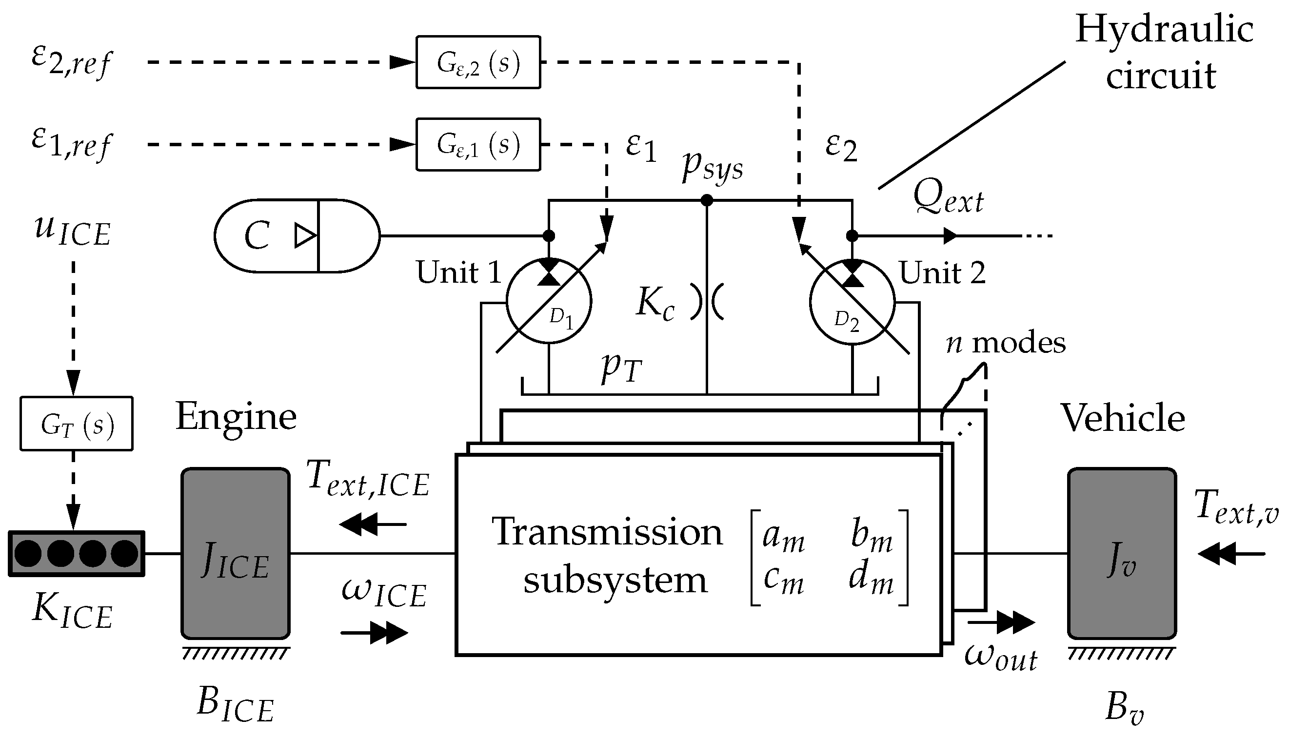
This section presents a linear lumped-parameter model used for the derivation of the decoupling strategy. The model is expressed in the frequency domain in accordance to Merritt [26] and was derived by the authors in [8]. Figure 1 shows the model with defined states ($p_{sys},{\omega }_{out},{\omega }_{ICE}$), control signals (${\epsilon }_{1,ref},{\epsilon }_{2,ref},u_{ICE}$), and disturbances ($Q_{ext},T_{ext,ICE},T_{ext,v}$). As previously mentioned, it describes the transmission within a mode m, and no clutches are therefore shown in the figure. The following major assumptions are made:

• The tank pressure, $p_T\approx 0$, is constant.
• Both hydraulic units may realize four-quadrant operation, i.e., ${\epsilon }_{1/2}\in [-1,1]$.
• The hydraulic circuit capacitance is dominated by that of the accumulator, C, and is high.
• The accumulator operates within minimum and maximum pressure levels (i.e., it is never empty).
• The fluid’s inertia and the effects of fluid line dynamics are negligible at the frequencies of interest.
• All mechanical inertia is concentrated at the engine ($J_{ICE}$) and the vehicle ($J_v$).
• The engine operates at idling speed or above at all times.
• The transmission subsystem is lossless, and each mode, m, is constituted by one of the basic single-mode configurations previously described.

As a result of the last assumption, the kinematic relationship between the transmission shafts may be be modeled using the following matrix description [27,28]:

$$\left[\begin{array}{c}{\omega }_1\\ {\omega }_2\end{array}\right]=\left[\begin{array}{cc}{a}_m& b_m\\ c_m& d_m\end{array}\right]\left[\begin{array}{c}{\omega }_{ICE}\\ {\omega }_{out}\end{array}\right],\left[\begin{array}{c}{T}_{ICE}\\ T_{out}\end{array}\right]=-{\left[\begin{array}{cc}{a}_m& b_m\\ c_m& d_m\end{array}\right]}^t\left[\begin{array}{c}{T}_1\\ T_2\end{array}\right]=\left[\begin{array}{cc}-a_m& -c_m\\ -b_m& -d_m\end{array}\right]\left[\begin{array}{c}{T}_1\\ T_2\end{array}\right]$$

(1)

An equivalent description has previously been used for the optimization and control of power-split hybrid HMTs for passenger vehicles [3,13]. The values of $a_m,b_m,c_m$ and $d_m$ are consequences of the gear ratios and planetary gear constants active in mode m. Furthermore, as a result of the last assumption above, $a_m\ne 0$ and $d_m\ne 0$. The model in Equation (1) may then be used to conveniently describe the ICPS ($b_m=0,c_m\ne 0$), OCPS ($b_m\ne 0,c_m=0$), and compound architectures ($b_m\ne 0,c_m\ne 0$). A series hybrid configuration is described with $b_m=c_m=0$.

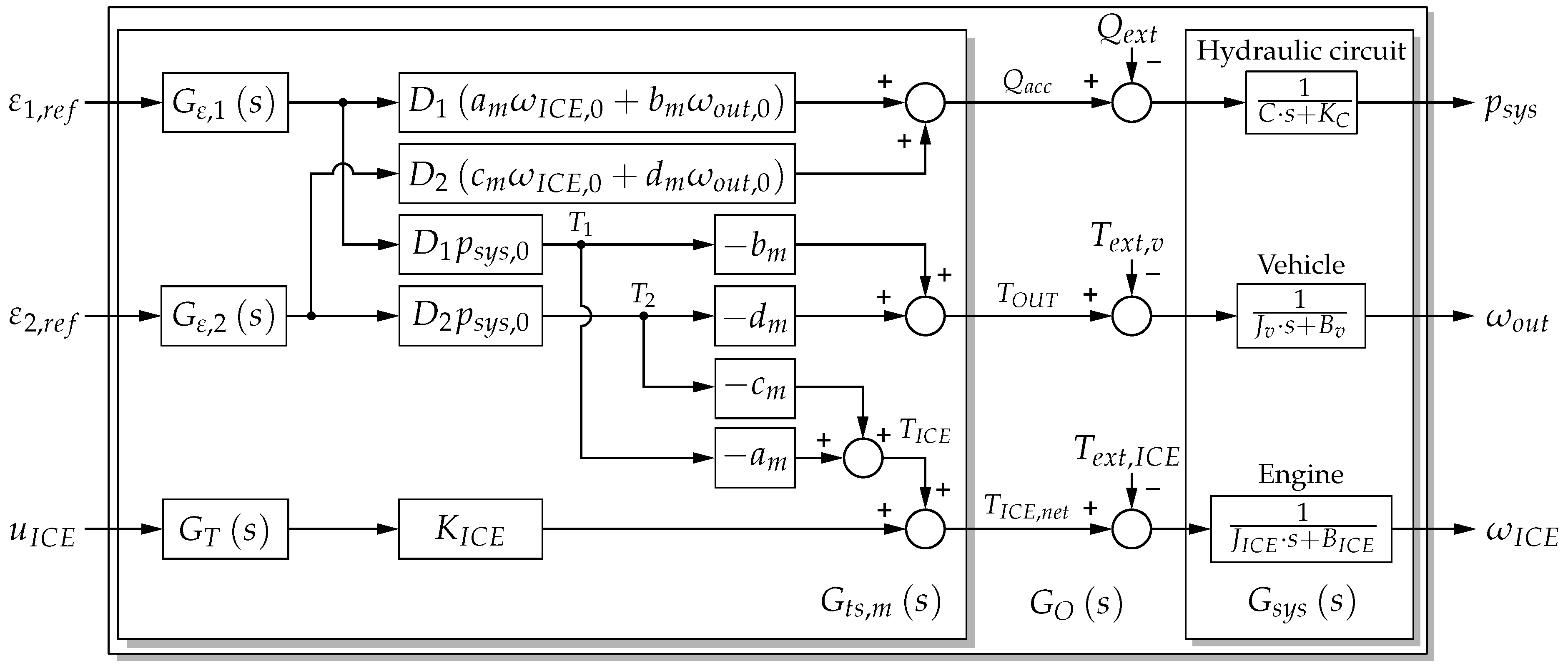
The causal effects of the input signals and the disturbances on the states in the model in Figure 1 are illustrated by the block diagram in Figure 2. It may be observed that the transmission subsystem ($a_m,b_m,c_m,d_m$) introduces cross-couplings between $p_{sys}$ and ${\omega }_{out}$, which are affected by changes in both ${\epsilon }_{1,ref}$ and ${\epsilon }_{2,ref}$. ${\omega }_{ICE}$ is affected by all control signals. However, since there is no path from $u_{ICE}$ to $p_{sys}$ and ${\omega }_{out}$, the engine is not subject to cross-couplings, but rather interferences from ${\epsilon }_{1,ref}$ and ${\epsilon }_{2,ref}$. In terms of instability, cross-couplings introduce hidden feedback loops that may cause problems in MIMO systems [24].

In the frequency domain, the model is described as:

$$\left[\begin{array}{c}{p}_{sys}\\ {\omega }_{out}\\ {\omega }_{ICE}\end{array}\right]=G_O\left(s\right)\left[\begin{array}{c}{\epsilon }_{ref,1}\\ {\epsilon }_{ref,2}\\ u_{ICE}\end{array}\right]-\left[\begin{array}{ccc}\frac{1}{Cs+K_C}& 0& 0\\ 0& \frac{1}{J_{v}s+B_v}& 0\\ 0& 0& \frac{1}{J_{ICE}s+B_{ICE}}\end{array}\right]\left[\begin{array}{c}{Q}_{ext}\\ T_{ext,v}\\ T_{ext,ICE}\end{array}\right]$$

(2)

where $G_O\left(s\right)$ is the open loop transfer function matrix:

$$G_O\left(s\right)=\left[\begin{array}{ccc}\frac{D_1\left(a_m{\omega }_{ICE,0}+b_m{\omega }_{out,0}\right)G_{\epsilon ,1}\left(s\right)}{Cs+K_C}& \frac{D_2\left(c_m{\omega }_{ICE,0}+d_m{\omega }_{out,0}\right)G_{\epsilon ,2}\left(s\right)}{Cs+K_C}& 0\\ -\frac{b_m{D}_1{p}_{sys,0}{G}_{\epsilon ,1}\left(s\right)}{J_{v}s+B_v}& -\frac{d_m{D}_2{p}_{sys,0}{G}_{\epsilon ,2}\left(s\right)}{J_{v}s+B_v}& 0\\ -\frac{a_m{D}_1{p}_{sys,0}{G}_{\epsilon ,1}\left(s\right)}{J_{ICE}s+B_{ICE}}& -\frac{c_m{D}_2{p}_{sys,0}{G}_{\epsilon ,2}\left(s\right)}{J_{ICE}s+B_{ICE}}& \frac{K_{ICE}{G}_T\left(s\right)}{J_{ICE}s+B_{ICE}}\end{array}\right]$$

(3)

For the decoupling strategy, it is convenient to factorize $G_O\left(s\right)$ according to:

$$G_O\left(s\right)=G_{sys}\left(s\right)G_{ts,m}\left(s\right)$$

(4)

where $G_{sys}\left(s\right)$ is a diagonal matrix that contains the governing dynamics of each state:

$$G_{sys}\left(s\right)=\left[\begin{array}{ccc}\frac{1}{Cs+K_C}& 0& 0\\ 0& \frac{1}{J_{v}s+B_v}& 0\\ 0& 0& \frac{1}{J_{ICE}s+B_{ICE}}\end{array}\right]$$

(5)

and $G_{ts,m}\left(s\right)$ contains the cross-couplings:

$$G_{ts,m}\left(s\right)=\left[\begin{array}{ccc}{D}_1\left(a_m{\omega }_{ICE,0}+b_m{\omega }_{out,0}\right)G_{\epsilon ,1}\left(s\right)& D_2\left(c_m{\omega }_{ICE,0}+d_m{\omega }_{out,0}\right)G_{\epsilon ,2}\left(s\right)& 0\\ -b_m{D}_1{p}_{sys,0}{G}_{\epsilon ,1}\left(s\right)& -d_m{D}_2{p}_{sys,0}{G}_{\epsilon ,2}\left(s\right)& 0\\ -a_m{D}_1{p}_{sys,0}{G}_{\epsilon ,1}\left(s\right)& -c_m{D}_2{p}_{sys,0}{G}_{\epsilon ,2}\left(s\right)& K_{ICE}{G}_T\left(s\right)\end{array}\right]$$

(6)

In previous work by the authors [29], it was found that the displacement controllers may be represented by second order transfer functions:

$$\left\{\begin{array}{c}\frac{{\epsilon }_1}{{\epsilon }_{1,ref}}=G_{\epsilon ,1}\left(s\right)=\frac{1}{\frac{s^2}{{\omega }_{a,1}^2}+2\frac{{\delta }_{a,1}}{{\omega }_{a,1}}s+1}\hfill \\ \frac{{\epsilon }_2}{{\epsilon }_{2,ref}}=G_{\epsilon ,2}\left(s\right)=\frac{1}{\frac{s^2}{{\omega }_{a,2}^2}+2\frac{{\delta }_{a,2}}{{\omega }_{a,2}}s+1}\hfill \end{array}\right.$$

(7)

The turbo dynamics are modeled according to [30]:

$$G_T\left(s\right)=\frac{{\tau }_{T}s+1}{\frac{{\tau }_T}{K_{\tau }}s+1}$$

(8)

3. Control

Before the decoupling strategy is derived, it is important to note that its implementation relies on a number of assumptions in addition to those previously listed:

• Although dynamic decoupling is possible [24], static decoupling is considered enough here.
• The configuration and, consequently, the constants ($a_m,b_m,c_m,d_m$) are known for all modes.
• The system pressure, $p_{sys}$, and engine speed ${\omega }_{ICE}$ are kept within allowed limits by the high-level controller.
• The displacement controllers are equally fast. This condition may be fulfilled with pre-filtering of the control signals or using the displacement control strategy in [29].

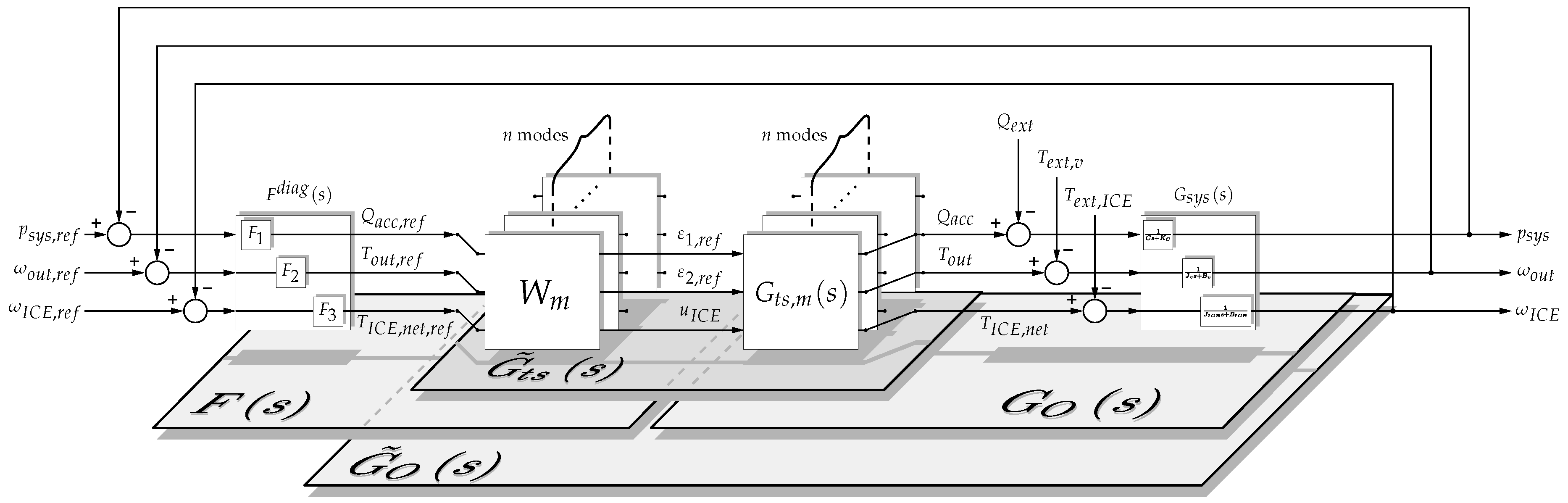
3.1. Decoupled MIMO-Control

Figure 3 illustrates the decoupled control strategy proposed in this paper. The full controller, $F\left(s\right)$, is divided into a diagonal part, $F^{diag}\left(s\right)$, and a decoupling matrix, $W_m$. For a transmission with n modes, n matrices, $W_m$, have to be defined, one for each mode m:

$$F\left(s\right)=W_m{F}^{diag}\left(s\right)$$

(9)

$$F^{diag}\left(s\right)=\left[\begin{array}{ccc}{F}_1\left(s\right)& 0& 0\\ 0& F_2\left(s\right)& 0\\ 0& 0& F_3\left(s\right)\end{array}\right]$$

(10)

$W_m$ may be found by putting requirements on the resulting transfer function matrix ${\tilde{G}}_{ts}\left(s\right)$:

$${\tilde{G}}_{ts}\left(s\right)=G_{ts,m}\left(s\right)W_m$$

(11)

As illustrated in Figure 2 and Figure 3, the output from $G_{ts,m}$ is the net accumulator flow $Q_{acc}$, the net output torque $T_{out}$, and the net engine torque $T_{ICE,net}$. The decoupling may then by realized by choosing a set of “fictive” control signals corresponding to these outputs. This is equivalent to requiring ${\tilde{G}}_{ts}\left(s\right)$ equal to identity:

$${\tilde{G}}_{ts}\left(s\right)=I$$

(12)

Considering Assumption 1, $W_m$ is chosen to fulfil the requirement in Equation (12) in the steady-state:

$$W_m=G_{ts,m}^{-1}\left(0\right)=\left[\begin{array}{ccc}\frac{d_m}{\left(a_m{d}_m-b_m{c}_m\right)D_1{\omega }_{ICE,0}}& \frac{c_m{\omega }_{ICE,0}+d_m{\omega }_{out,0}}{\left(a_m{d}_m-b_m{c}_m\right)D_1{p}_{sys,0}{\omega }_{ICE,0}}& 0\\ \frac{b_m}{\left(b_m{c}_m-a_m{d}_m\right)D_2{\omega }_{ICE,0}}& \frac{a_m{\omega }_{ICE,0}+b_m{\omega }_{out,0}}{\left(b_m{c}_m-a_m{d}_m\right)D_2{p}_{sys,0}{\omega }_{ICE,0}}& 0\\ \frac{p_{sys,0}}{K_{ICE}{\omega }_{ICE,0}}& \frac{{\omega }_{out,0}}{K_{ICE}{\omega }_{ICE,0}}& \frac{1}{K_{ICE}}\end{array}\right]$$

(13)

Assumption 4 yields:

$$G_{\epsilon ,1}\left(s\right)=G_{\epsilon ,2}\left(s\right)=G_{\epsilon }\left(s\right)=\frac{1}{\frac{s^2}{{\omega }_a^2}+2\frac{{\delta }_a}{{\omega }_a}s+1}$$

(14)

This results in the following decoupled open loop transfer function, ${\tilde{G}}_O\left(s\right)$:

$${\tilde{G}}_O\left(s\right)=G_O\left(s\right)W_m=\left[\begin{array}{ccc}\frac{G_{\epsilon }\left(s\right)}{Cs+K_C}& 0& 0\\ 0& \frac{G_{\epsilon }\left(s\right)}{J_{v}s+B_v}& 0\\ \frac{p_{Ssys,0}\left(G_T\left(s\right)-G_{\epsilon }\left(s\right)\right)}{{\omega }_{ICE,0}\left(J_{ICE}s+B_{ICE}\right)}& \frac{w_{out,0}\left(G_T\left(s\right)-G_{\epsilon }\left(s\right)\right)}{{\omega }_{ICE,0}\left(J_{ICE}s+B_{ICE}\right)}& \frac{G_T\left(s\right)}{J_{ICE}s+B_{ICE}}\end{array}\right]$$

(15)

The following should be noted concerning $W_m$ and ${\tilde{G}}_O\left(s\right)$:

• $W_m$ contains linearization points of pressure and shaft speeds. Consequently, gain scheduling is required to ensure that ${\tilde{G}}_O\left(s\right)$ according to Equation (15) is achieved.
• ${\tilde{G}}_O\left(s\right)$ is independent of mode m.
• Since $W_m$ is static, the difference between the displacement controller dynamics and turbo dynamics causes dynamic disturbances in the engine control loop.

The Diagonal Controller

$F^{diag}\left(s\right)$ is chosen based on the diagonal elements of ${\tilde{G}}_O\left(s\right)$. Here, simple proportional controllers are considered to illustrate the distinguishing features of the decoupled control strategy:

$$F^{diag}\left(s\right)=F^{diag}=\left[\begin{array}{ccc}{K}_1& 0& 0\\ 0& K_2& 0\\ 0& 0& K_3\end{array}\right]$$

(16)

As explained in [8], stability in the resulting SISO loops may occur in the pressure and output speed loop, but not in the engine speed loop, leading to the following upper limits on $K_1$ and $K_2$:

$$\left\{\begin{array}{c}{K}_1<2C{\delta }_a{\omega }_a\hfill \\ K_2<2J_v{\delta }_a{\omega }_a\hfill \end{array}\right.$$

(17)

Depending on its exact implementation, the pressure controller may be interpreted as part of the high-level controller, which sets the accumulator flow to achieve a desired pressure [3]. Similarly, the controller for the output speed loop may be interpreted as the operator who controls the output speed by adjusting the output torque [18].

The optimal choice of $K_{1/2/3}$ is not within the scope of this paper, and for the reference vehicle, the values were chosen to achieve acceptable response with sufficient margins in relation to Equation (17), while still being reproducible by the HWIL simulation setup. An attempt to choose the gains based on pole-placement was made in [8].

3.2. Baseline

The baseline approach is to apply a diagonal controller based solely on the diagonal elements of $G_O\left(s\right)$, thereby ignoring the cross-couplings. To make the responses of the two controllers comparable, this diagonal controller is chosen as the diagonal elements of $F\left(s\right)$ for the decoupled controller:

$$F_{BL}=\left[\begin{array}{ccc}{K}_1\frac{d_m}{\left(a_m{d}_m-b_m{c}_m\right)D_1{\omega }_{ICE,0}}& 0& 0\\ 0& K_2\frac{a_m{\omega }_{ICE,0}+b_m{\omega }_{out,0}}{\left(b_m{c}_m-a_m{d}_m\right)D_2{p}_{sys,0}{\omega }_{ICE,0}}& 0\\ 0& 0& K_3\frac{1}{K_{ICE}}\end{array}\right]$$

(18)

where the same controller gains $K_{1/2/3}$ and gain-scheduling of pressure and shaft speeds as in the decoupled strategy are used.

4. Reference Vehicle

The primary target for this control approach is larger wheel loaders with multiple-mode transmissions. However, the focus in this paper is on the control within a mode, and therefore, a compact wheel loader and a single-mode transmission were chosen and dimensioned to match the test rig and its power limitations. The vehicle parameters are given in

Table 1. Parameters for the reference vehicle.

Parameter	Value
Vehicle mass	5500 kg
Maximum speed	30 km/h
Maximum tractive force	50 kN
Max engine power	52.7 kW

.

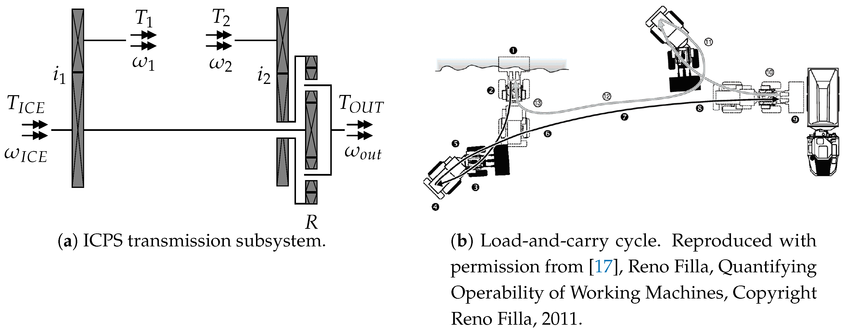
The reference transmission, shown in Figure 4a, was of the ICPS type. For this configuration, the transmission subsystem constants may be identified according to:

$$\left[\begin{array}{cc}{a}_m& b_m\\ c_m& d_m\end{array}\right]=\left[\begin{array}{cc}{i}_1& 0\\ \frac{1}{i_{2}R}& \frac{R-1}{i_{2}R}\end{array}\right]$$

(19)

The reference vehicle was simulated for two drive cycles. The first one was a simplified version of the load-and-carry cycle [17], shown in Figure 4b. In the load-and-carry cycle, the wheel loader enters a gravel pile to fill the bucket in low velocity, reverses, and then travels with higher velocity to a load receiver to empty the bucket. The aim with the simulation of this cycle was to study the principal operation of the decoupled control for a realistic case with relatively slow dynamics.

The second cycle was a series of steps in reference and disturbance signals. This case was not as realistic as the simplified load-and-carry cycle, but here, the aim was to study the dynamic couplings in the system and the effect of disturbances from additional power consumers, such as work functions.

5. Hardware-in-the-Loop Simulations

This section briefly presents the HWIL simulation setup and the model used to test the two control strategies applied on the reference vehicle for the two cycles. See [31] for a more detailed discussion on the aspects considered in the implementation of the simulation setup. The simulation model was explained in more detail in [8].

5.1. Test Rig

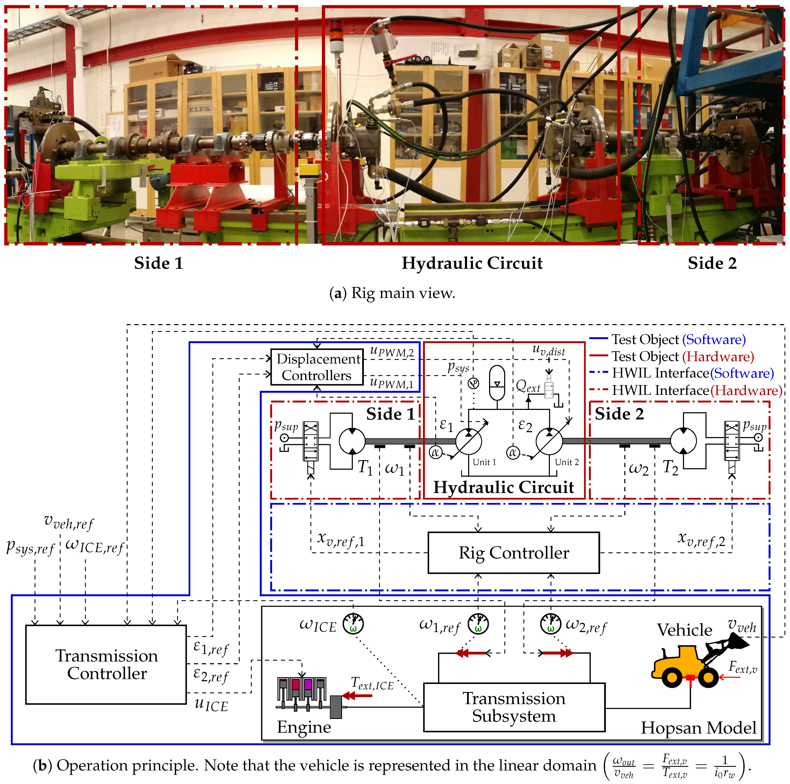
Figure 5 shows an overview of the test rig used in the HWIL simulations. Its principal-of-operation is shown in Figure 5b. In accordance with the HWIL simulation principle, the hydraulic circuit of the vehicle was replaced by hardware, while its surroundings were simulated by a model executed in real time. This was enabled by an HWIL interface connected between the model and the hydrostatic units in the hydraulic circuit. The interface contained a substantial power amplification, thereby classifying the test setup as power-HWIL [32]. Through this interface, the shaft torques were measured and sent to the model, which in turn, calculated the corresponding shaft speeds. These values were sent as reference values to the rig controller, which controlled the actual shaft speeds in closed loop. This control was enabled by a servo valve-controlled hydraulic motor connected to each hydraulic circuit unit. The rig control strategy was based on PI-control and feed-forward of the reference speed. In addition, a disturbance rejection strategy was used to compensate for the disturbances caused by the change in displacement of the hydrostatic units [31].

5.1.1. Hydraulic Circuit

The hydraulic circuit contained two Bosch Rexroth A11VO axial piston units of the in-line design with maximum displacement of 110 cm${}^3$/revolution. These units were connected in an open circuit with a common tank on the low-pressure side and two 20-L Hydac piston accumulators pre-charged at 90 bar at the high-pressure side. A Moog D769 servo valve was connected at the high-pressure side to simulate the effect of a flow disturbance.

The displacement of each unit was varied by an internal hydromechanical actuator fed from the circuit’s high pressure side. A Pulse-Width-Modulated (PWM) voltage signal actuated a proportional control valve that varied the flow to pistons acting on the unit’s swash plate. The swash plate angle was measured with a Hall-effect sensor and was then used for external closed-loop control of the displacement setting. A model of the displacement actuator was derived in [33], and a control strategy using a lead-compensator and pole-placement was proposed and tested in [29]. The same strategy was used in this paper, with additional gain-scheduling to compensate for the pressure-dependent change in static loop gain.

5.1.2. Data Acquisition System

In the test rig, the real-time calculations were carried out with a PXI-8110-RT real-time computer from National Instruments (NI) that ran LabVIEW${}^{\mathrm{TM}}$ as a server in real-time at a frequency of 1 kHz. The real-time computer measured/sent the signals from/to the rig sensors/actuators through an NI PXI-7813R FPGA board connected to a set of NI module measurement cards. Amplification of PWM signals and voltage output signals and signal conditioning were carried out with a set of Prevas Gobi FISC (Fault Injection Signal Conditioning) boards. Controllers and models were implemented as compiled Simulink and Hopsan models that were uploaded to the server offline.

5.2. Hopsan Model

The model used to describe the surroundings of the hydraulic circuit was implemented in Hopsan, a system simulation tool developed at Linköping University [34]. This software is based on the Transmission Line element Method (TLM), which considers the constant time delays present in physical elements [35].

The engine was modeled according to the Mean-Value-Engine-Modeling (MVEM) principle [36] and contained, in addition to the flywheel and turbo dynamics previously described, a second-order polynomial friction model and a maximum torque-curve from a conventional wheel-loader engine [37]. Both the friction model and the maximum torque curve were scaled to fit the reference vehicle using Mean Effective Pressure (MEP) scaling laws [8].

The vehicle was modeled as a one-dimensional moving mass subjected to constant rolling resistance, speed-dependent shaft losses, and constant final gear efficiency [8,38].

The transmission subsystem was modeled using shaft and gear components in Hopsan. The gears were modeled as static components with constant efficiencies. The shafts were modeled as TLM elements in the rotational domain (i.e., springs) with additional numerical damping. TLM spring elements are, in addition to the spring stiffness, subject to parasitic inductance [35]. Here, this property represented the rotational inertias of the shaft/gear combinations.

For the load-and-carry cycle, a simple model was used to simulate the force acting on the wheel loader when it entered the gravel pile. The model was based on empirical data and assumed an exponential increase of resistive force depending on the distance traveled into the pile [39].

6. Results

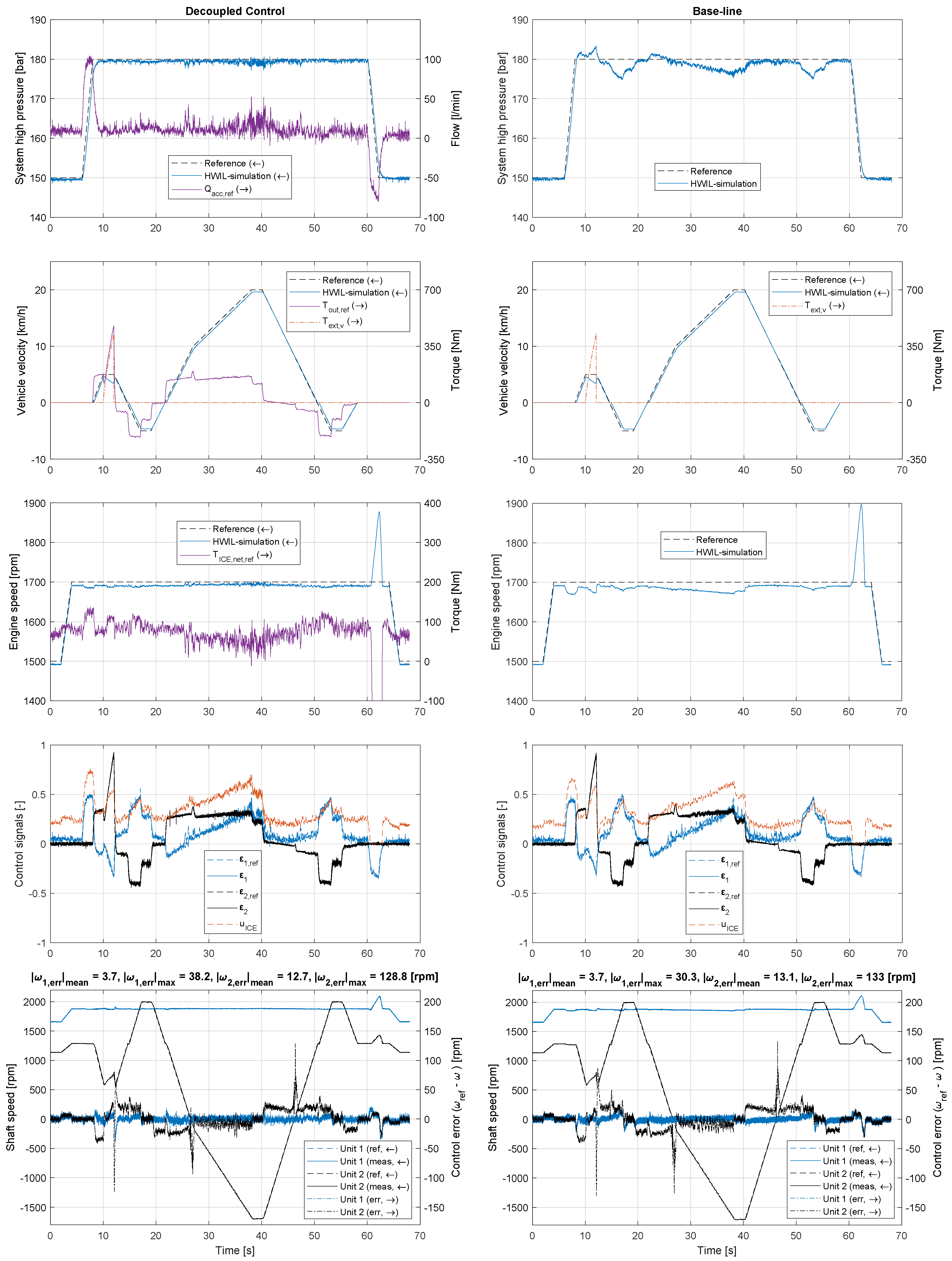
Model parameter values and other settings used during the experiments are given in Appendix A. The reference and disturbance signals for the drive cycles were first defined offline in time-dependent vectors and then sent as input to the controllers during the tests. Figure 6 shows the HWIL-simulation of the load-and-carry cycle, while the step-series cycle is shown in Figure 7.

6.1. Load-and-Carry Cycle

The basic idea of the decoupled control strategy is that each state is controlled by a decoupled control signal. For instance, in the measurements the system pressure was controlled by the desired net accumulator flow, $Q_{acc,ref}$, which primarily reacted to a change in reference pressure (at 6–8 s and 60–62 s). Similarly, the desired output torque, $T_{out,ref}$, was altered to follow the speed reference. The gravel pile may be observed as a peak in torque and a drop in vehicle speed at 10–12 s. At the lowest level, however, all control signals (${\epsilon }_{1,ref},{\epsilon }_{2,ref},u_{ICE}$) changed simultaneously to handle the cross-couplings. For instance, Unit 2 determined the transmission output torque through variations in ${\epsilon }_2$, which also results in a flow that must be received by Unit 1 for a maintained zero accumulator flow. As previously discussed, the engine was subject to dynamic disturbances from the other loops (see Equation (15)), which may be observed as drops in engine speed when the accumulator is filled and when the gravel pile is entered. When the accumulator was emptied (at 60–62 s), a peak in engine speed may be observed, which was caused by the accumulator energy being burnt as engine friction.

In contrast to the decoupled strategy, the baseline approach was limited to handling the cross-couplings using its state feedbacks and gain-scheduling. Consequently, steady-state errors were present in the engine and pressure loops. The vehicle speed reference tracking performance was very similar for the two strategies. This was because the output torque of an ICPS transmission was determined by the torque of Unit 2 alone ($b_m=0$), thereby making the vehicle speed loop naturally decoupled.

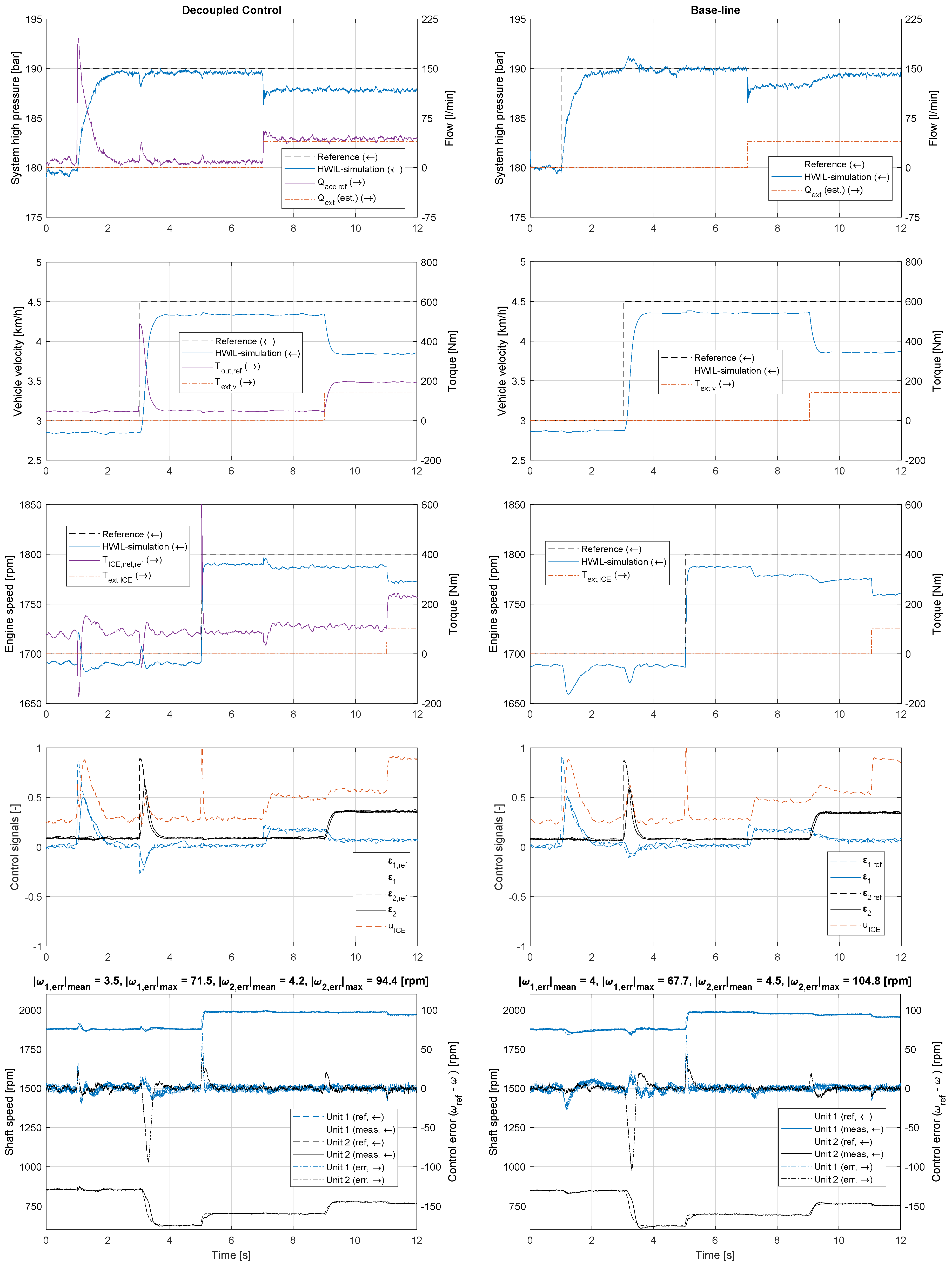
6.2. Step-Series Cycle

This cycle was a series of steps in each state and disturbance signal. For the decoupled strategy, the presence of dynamic disturbances in the engine speed loop may be observed at one and three seconds as steps were made in pressure and vehicle speed. In the pressure loop, a similar disturbance occurred at three seconds, when a step was made in vehicle velocity. This behavior was not predicted by the linear model (see Equation (15)) and is explained by the displacement actuators not being equally fast in reality [8], primarily due to saturation in the flow of the actuators for larger step magnitudes [29].

The external disturbances caused steady-state errors in all loops, since these were not known by the decoupling strategy. In the engine speed loop, a small disturbance may also be observed at seven seconds as the pressure loop compensated for its flow disturbance.

The differences between the baseline and decoupled strategies were confirmed further in this cycle. The engine was subject to more severe disturbances caused by the other states and also suffered from additional static error as the disturbances were introduced in the other states. One phenomenon that may be observed in the pressure loop was that the steady-state error was lowered as the torque disturbance was introduced in the vehicle speed loop. This was because the increased displacement of Unit 2 caused an extra flow into the circuit, which compensated for the external disturbance flow.

7. Discussion

Compared to the decoupled control strategy, the baseline approach suffers from steady-state errors since it cannot predict the disturbances caused by the system’s internal cross-couplings. Naturally, this problem could be handled by integrating elements in the controller. This would, however, introduce phase lag and thus have a negative impact on stability. More importantly, the integrators would have a negative effect on the functionality in the case of multiple-mode transmissions. In these systems, the transmission kinematics change in between the modes, which means that integrator wind-up needs to be handled to ensure smooth mode shifts [25]. In the decoupled approach, however, the decoupling matrix takes care of this issue in a feed-forward manner. Furthermore, the decoupled strategy automatically manages the driver’s torque control, which depends strongly on the transmission configuration [13]. The decoupled strategy also automatically handles the rejection of the disturbances that act on the ICE, which otherwise usually is carried out in an individual engine control loop [3,15]. It should be noted that the control strategy in itself does not guarantee energy-efficient performance of the machine. For instance, it is not rational to empty the accumulator when the vehicle is standing still, thereby causing the engine to speed up. In a final implementation, a high-level strategy is needed to ensure the accumulator is utilized in a fuel-efficient manner [3]. Furthermore, the desired output torque needs to be blended with the friction brakes during vehicle braking [2].

Some extensions are natural to make for the proposed control strategy to consider the complete machine. For instance, the external disturbances, $Q_{ext}$ and $T_{ext,ICE}$, should be extended to consider the work functions with their operator input signals, actuators, and states. These could be implemented as a working hydraulics system on the engine ($T_{ext,ICE}$), as is the case in a conventional wheel loader [17] or as a secondary controlled system connected to the hydraulic circuit ($Q_{ext}$) [6]. An additional aspect for wheel loaders is that the load (i.e., gravel pile) connects the transmission and the work functions during bucket-filling [17]. A cross-coupling between $T_{ext,v}$ and the work functions is therefore to be expected in this phase. Another extension is to enhance the considered ICE properties. Typically, this enhancement would be to include intake manifold pressure as a state and thereby enable more exact modeling of the turbo dynamics’ and “smoke-limiter’s” effects on the engine response and fuel consumption [40]. Furthermore, the friction losses in the hydraulic units and the transmission subsystem could have an influence on the control in some configurations and may then need to be considered in the control strategy [41].

In addition to these effects, other non-linearities that change the dynamics are present in the real system. Primarily, these are saturation in control signals, such as limited engine torque, limited displacement, and displacement actuator velocity [8]. The limitation in displacement actuator velocity, due to limited actuator flow [33], causes the displacement controllers of Units 1 and 2 to be unequally fast for different step magnitudes, which was observed as dynamic cross-couplings in the experiments carried out in this paper. Another non-linear effect is that the hydraulic capacitance decreases for increased pressures. This effect was found to be larger in simulations [8] than in the experiments carried out here. The capacitance is, however, directly related to the stability of the pressure loop (see Equation (17)), and this effect should therefore be taken into account when designing the pressure controller.

The decoupled control strategy proved to be beneficial for the reference single-mode ICPS hybrid HMT. A logical next step would, however, be to consider other HMT configurations and multiple-mode concepts. For instance, the OCPS configuration ($c_m=0,b_m\ne 0$) contains cross-couplings between the vehicle speed and system pressure loops, which would probably affect the torque control [13]. When it comes to multiple-mode concepts, the mode shifting event introduces an additional control problem to handle. This concerns both the combination of clutch timing and displacement controller response [25], as well as the effect of pump/motor losses on the change of power flow direction in the hydraulic circuit [38].

In MIMO systems, the presence of cross-couplings may lead to instability in some cases [24]. For the reference vehicle studied in this paper, such tendencies have not been observed, and the stable nature of the baseline strategy confirms this further. For other transmission configurations, and extended versions of the strategy according to the above, a study of the severity of the cross-couplings could be motivated; see for instance [42]. Since static decoupling was considered, dynamic disturbances occurred in the measurements. For the application considered in this paper, these disturbances were considered acceptable. If required, however, dynamic decoupling could be considered, which would require accurate models of the displacement controller and turbo dynamics. Concerning the diagonal controller, proportional elements were used in the experiments. Depending on the requirements on the closed loops, however, more sophisticated controllers could be considered. For example, the steady-state error caused by friction, leakage, and external disturbances could be handled with integrating elements.

8. Conclusions

In contrast to the baseline approach, the proposed decoupled control strategy canceled out the cross-couplings present in a complex hybrid hydromechanical transmission. The steady-state errors caused by these cross-couplings were thus eliminated in a feed-forward manner rather than using integrating elements. This feature, combined with being based on a general model of a complex transmission subsystem, motivates a future application of the strategy on multiple-mode transmissions. Furthermore, torque control was achieved in a convenient way, which typically is required from an operator’s perspective.

The strategy may be extended to consider additional machine power consumers, such as work functions, and is intended as an enabler and facilitator for the implementation of high-level control strategies in fuel-efficient heavy mobile working machines.

References

- Filla, R. Hybrid Power Systems for Construction Machinery: Aspects of System Design and Operability of Wheel Loaders. In Proceedings of the ASME 2009 International Mechanical Engineering Congress and Exposition Volume 13: New Developments in Simulation Methods and Software for Engineering, Lake Buena Vista, FL, USA, 13–19 November 2009. [Google Scholar] [CrossRef]
- Guzella, L.; Sciaretta, A. Vehicle Propulsion Systems; Springer: Berlin/Heidelberg, Germany, 2013. [Google Scholar] [CrossRef]
- Cheong, K.L.; Du, Z.; Li, P.Y.; Chase, T.R. Hierarchical control strategy for a hybrid hydromechanical transmission (HMT) power-train. In Proceedings of the American Control Conference, Portland, OR, USA, 4–6 June 2014. [Google Scholar] [CrossRef]
- Karbaschian, M.A.; Söffker, D. Review and Comparison of Power Management Approaches for Hybrid Vehicles with Focus on Hydraulic Drives. Energies 2014, 7, 3512–3536. [Google Scholar] [CrossRef]
- Wang, F.; Mohd Zulkefli, M.A.; Sun, Z.; Stelson, K.A. Energy management strategy for a power-split hydraulic hybrid wheel loader. Proc. Inst. Mech. Eng. Part D J. Automob. Eng. 2015. [Google Scholar] [CrossRef]
- Pettersson, K.; Heybroek, K.; Mattsson, P.; Krus, P. A novel hydromechanical hybrid motion system for construction machines. Int. J. Fluid Power 2016. [Google Scholar] [CrossRef]
- Uebel, K.; Raduenz, H.; Krus, P.; de Negri, V. Design Optimisation Strategies for a Hydraulic Hybrid Wheel Loader. In Proceedings of the BATH/ASME 2018 Symposium on Fluid Power and Motion Control, Bath, UK, 12–14 September 2018. [Google Scholar] [CrossRef]
- Larsson, L.V.; Krus, P. A General Approach to Low-Level Control of Heavy Complex Hybrid Hydromechanical Transmissions. In Proceedings of the BATH/ASME 2018 Symposium on Fluid Power and Motion Control, Bath, UK, 12–14 September 2018. [Google Scholar] [CrossRef]
- Nikolaus, H. Hydrostatische Fahr- und Windenantriebe mit Energierückgewinnung. Ölhydraul. Pneumat. 1981, 25, 193–194. [Google Scholar]
- Palmgren, G. On Secondary Controlled Hydraulic Systems. Lic. Thesis, Linköping University, Linköping, Sweden, 1988. [Google Scholar]
- Kordak, R. Hydrostatic Drives with Secondary Control; Mannesmann Rexroth GmbH: Lohr am Main, Gwemany, 1996. [Google Scholar]
- Berg, H.; Ivantysynova, M. Design and testing of a robust linear controller for secondary controlled hydraulic drive. Proc. Inst. Mech. Eng. Part I J. Syst. Control Eng. 1999, 213, 375–386. [Google Scholar] [CrossRef]
- Cheong, K.L.; Li, P.Y.; Sedler, S.; Chase, T.R. Comparison between Input Coupled and Output Coupled Power-split Configurations in Hybrid Vehicles. In Proceedings of the 52nd National Conference on Fluid Power, Milwaukee, WI, USA, 23–25 March 2011; pp. 243–252. [Google Scholar]
- Hugosson, C. Cumulo Hydrostatic Drive—A Vehicle Drive with Secondary Control. In Proceedings of the Third Scandinavian International Conference on Fluid Power, Linköping, Sweden, 3–5 June 1993; pp. 475–494. [Google Scholar]
- Kumar, R.; Ivantysynova, M. An Optimal Power Management Strategy for Hydraulic Hybrid Output Coupled Power-Split Transmission. In Proceedings of the ASME 2009 Dynamic Systems and Control Conference, Hollywood, CA, USA, 12–14 October 2009. [Google Scholar] [CrossRef]
- Li, P.Y.; Mensing, F. Optimization and Control of a Hydro-Mechanical Transmission based Hybrid Hydraulic Passenger Vehicle. In Proceedings of the 7th International Fluid Power Conference, Aachen, Germany, 22–24 March 2009. [Google Scholar]
- Filla, R. Quantifying Operability of Working Machines. Ph.D. Thesis, Linköping University, Linköping, Sweden, 2011. [Google Scholar] [CrossRef]
- Mutschler, S.; Brix, N.; Xiang, Y. Torque Control for Mobile Machines. In Proceedings of the 11th International Fluid Power Conference, Aachen, Germany, 19–21 March 2018; pp. 186–195. [Google Scholar] [CrossRef]
- Anderl, T.; Winkelhake, J.; Scherer, M. Power-split Transmissions For Construction Machinery. In Proceedings of the 8th International Fluid Power Conference (IFK2012), Dresden, Germany, 22–24 March 2012; pp. 189–201. [Google Scholar]
- Carl, B.; Ivantysynova, M.; Williams, K. Comparison of Operational Characteristics in Power Split Continuously Variable Transmissions; SAE Technical Paper; SAE International: New York, NY, USA, 2006; pp. 776–790. [Google Scholar]
- Uebel, K. Conceptual Design of Complex Hydromechanical Transmissions. Ph.D. Thesis, Linköping University, Linköping, Sweden, 2017. [Google Scholar] [CrossRef]
- Kress, J.H. Hydrostatic Power-Splitting Transmissions for Wheeled Vehicles—Classification and Theory of Operation; SAE Technical Paper 680549; SAE International: New York, NY, USA, 1968. [Google Scholar]
- Glad, T.; Ljung, L. Reglerteknik: Flervariabla och Olinjära Metoder, 2nd ed.; Studentlitteratur AB: Lund, Sweden, 2003. [Google Scholar]
- Albertos, P.; Sala, A. Multivariable Control Systems; Springer: Berlin/Heidelberg, Germany, 2004. [Google Scholar]
- Larsson, L.V.; Pettersson, K.; Krus, P. Mode Shifting in Hybrid Hydromechanical Transmissions. In Proceedings of the ASME/BATH 2015 Symposium on Fluid Power and Motion Control (FPMC2015), Chicago, IL, USA, 12–14 October 2015. [Google Scholar] [CrossRef]
- Merritt, H.E. Hydraulic Control Systems; John Wiley & Sons, Inc.: Hoboken, NJ, USA, 1967. [Google Scholar]
- Mattsson, P. Continuously Variable Split-Power Transmissions with Several Modes. Ph.D. Thesis, Chalmers University of Technology, Göteborg, Sweden, 1996. [Google Scholar]
- Sanger, D. Matrix methods in the analysis and synthesis of coupled differentials and differential mechanisms. In Proceedings of the Fourth World Congress on the Theory of Machines and Mechanisms, Newcastle, UK, 8–12 September 1975; pp. 27–31. [Google Scholar]
- Larsson, L.V.; Krus, P. Displacement Control Strategies of an In-Line Axial-Piston Unit. In Proceedings of the 15th Scandinavian International Conference on Fluid Power, Linköping, Sweden, 7–9 June 2017; pp. 244–253. [Google Scholar]
- Lennevi, J.; Palmberg, J.O. The Significance for Control Design of the Engine and Power Transmission Coupling in Hydrostatic Drivetrains. In Proceedings of the 8th Bath International Fluid Power Workshop on Design and Performance, Bath, UK, 20–22 September 1995. [Google Scholar]
- Larsson, L.V.; Krus, P. Hardware-in-the-loop Simulation of Complex Hybrid Hydromechanical Transmissions. In Proceedings of the WIEFP2018-4th Workshop on Innovative Engineering for Fluid Power, Sao Paulo, Brazil, 28–30 November 2018. [Google Scholar] [CrossRef]
- Steurer, M.; Edrington, C.S.; Sloderbeck, M.; Ren, W.; Langston, J. A Megawatt-Scale Power Hardware-in-the-Loop Simulation Setup for Motor Drives. IEEE Trans. Ind. Electron. 2010, 57, 1254–1260. [Google Scholar] [CrossRef]
- Larsson, L.V.; Krus, P. Modelling of the Swash Plate Control Actuator in an Axial Piston Pump for a Hardware-in-the-Loop Simulation Test Rig. In Proceedings of the 9th FPNI Ph.D. Symposium on Fluid Power, Florianópolis, Brazil, 26–28 October 2016. [Google Scholar] [CrossRef]
- Linköping University, Division of Fluid and Mechatronic Systems. Hopsan. Available online: https://liu.se/en/research/hopsan/ (accessed on 26 April 2019).
- Braun, R. Distributed System Simulation Methods For Model-Based Product Development. Ph.D. Thesis, Linköping University, Linköping, Sweden, 2015. [Google Scholar] [CrossRef]
- Eriksson, L.; Nielsen, L. Modeling and Control of Engines and Drivelines; John Wiley & Sons Ltd.: Hoboken, NJ, USA, 2014. [Google Scholar] [CrossRef]
- Volvo Construction Equipment. Volvo L90H Wheel Loader, Product Brochure. Available online: https://www.volvoce.com/-/media/volvoce/global/products/wheel-loaders/compact-wheel-loader/brochures/brochure_l60h_l70h_l90h_t4f_sv_12_20045607_b.pdf?v=29AvPw (accessed on 26 April 2019).
- Larsson, L.V.; Larsson, K.V. Simulation and Testing of Energy Efficient Hydromechanical Drivelines for Construction Machinery. Master’s Thesis, Linköping University, Linköping, Sweden, 2014. [Google Scholar]
- Pettersson, K.; Larsson, L.V.; Larsson, K.V.; Krus, P. Simulation Aided Design and Testing of Hydromechanical Transmissions. In Proceedings of the 9th JFPS International Symposium on Fluid Power (JFPS14), Matsue, Japan, 28–31 October 2014. [Google Scholar]
- Nezhadali, V.; Sivertsson, M.; Eriksson, L. Turbocharger Dynamics Influence on Optimal Control of Diesel Engine Powered Systems. SAE Int. J. Engines 2014, 7, 6–13. [Google Scholar] [CrossRef]
- Hedman, A. Continuously Variable Split-Power Transmissions at Near-Zero Output Speeds. In Proceedings of the Eight World Congress on the Theory of Machines and Mechanisms, Prague, Czechoslovakia, 26–31 August 1991. [Google Scholar]
- Rosenbrock, H.H. Computer-Aided Control System Design; Academic Press Inc. Ltd.: London, UK, 1974. [Google Scholar]
Figure 1.
Linear lumped-parameter model of a general complex multi-mode hydraulic hybrid transmission with n modes, in mode m. and are disturbances caused by, for instance, work functions, while is a disturbance from a load, e.g., a gravel pile.
Figure 2.
Block diagram of the linear model in Figure 1 at mode m, linearized at .
Figure 3.
Schematic overview of a decoupled MIMO control approach for a complex hydraulic hybrid transmission with n modes.
Figure 4.
Reference vehicle transmission and drive cycle.
Figure 5.
Overview of the HWIL test rig used in the study.
Figure 6.
HWIL-simulation results of the load-and-carry cycle for decoupled (left column) and baseline (right column) control. and are zero for this cycle and are therefore not included in the graphs. Note that the bottom row shows the performance of the HWIL simulation controller and not the transmission control strategy. The output shaft speed has been scaled to vehicle velocity via the wheel radius and final gear ratio .
Figure 7.
HWIL-simulation results of the step series cycle for decoupled (left column) and baseline (right column) control. Note that the bottom row shows the performance of the HWIL simulation controller and not the transmission control strategy. The output shaft speed has been scaled to vehicle velocity via the wheel radius and final gear ratio . was estimated according to , where a step of 2.15 V was made in .