Evaluation of the Energy Supply Options of a Manufacturing Plant by the Application of the P-Graph Framework


1
Department of Computer Science and Systems Technology, University of Pannonia, 8200 Veszprém, Egyetem utca 10., Hungary
2
Institute for Process Systems Engineering and Sustainability, Pázmány Péter Catholic University, 1088 Budapest, Szentkirályi utca 28., Hungary
*
Author to whom correspondence should be addressed.
Energies 2019, 12(8), 1484; https://doi.org/10.3390/en12081484
Submission received: 4 February 2019
/
Revised: 11 April 2019
/
Accepted: 13 April 2019
/
Published: 18 April 2019
(This article belongs to the Special Issue Selected Papers from PRES 2018: The 21st Conference on Process Integration, Modelling and Optimisation for Energy Saving and Pollution Reduction)
Abstract
:Industrial applications nowadays are facing the complexity of the problem of finding an optimal energy supply composition. Heating and electricity needs vary throughout a year and need to be addressed. There is usually power available from the market, but a company has other investment options to consider, such as solar power, or utilization of local biomass. Fixed and proportional investment and operational costs must be compared to long-term cost-efficiency. The P-Graph framework is an effective tool in the design and synthesis of process networks, and is capable of showing optimal decisions. In the present work, a new P-Graph model was implemented to address the synthesis of the energy supply options of a manufacturing plant in Hungary. Compared to the original approach, a multi-periodic scheme was applied for heating and electricity demands. Also, the pelletizer and biogas plant investments are modeled in the P-Graph with a new technique that better reflects equipment capacities and flexible input ratios. The best solutions in this case study in terms of total costs are listed. It can be concluded that a long-term investment horizon is needed for the incorporation of sustainable energy sources into the system to be cost-efficient.
1. Introduction
1.1. Overview of the Present Work
Energy supply is one of the most important problems for modern industrial facilities. Usually, when a plant is built, it is connected to the grid allowing it to purchase electricity for its operation. The same holds for heating, water, or other requirements where public services are available. However, environmental regulations play an increasing role, and small to medium scale power plants are becoming popular. Such power sources have the ability to supply the needs of individual residential homes or firms. These can have significant investment costs, but operation in the long-term may make them cost-efficient solutions. There is no absolute winner technology in terms of costs.
The power supply decision can be a complex problem. Several different energy sources have to be taken into account. Renewable energy sources like biomass can have a limited availability and are usually neither economical nor environmentally friendly if they need to be transported over long distances. Different technologies and energy supply methods may coexist, but each having different investment and operational costs, for which capacity is also limited. Energy demands can also vary, not only from one year to the other, but even from month to month, according to the seasons. This is especially true for heating requirements.
The P-Graph framework is a modeling tool with which one can define Process Network Synthesis (PNS) problems. In a PNS, a system of complex possible flow of materials is given, and a cost-optimal selection of possible operating units must be found. The P-Graph framework consists of the mathematical model of P-Graphs, the corresponding theorems and algorithms, and also software in which we can solve PNS problems.
This work presents a case study made for a manufacturing plant, for which decision makers needed to consider alternative energy sources like solar power and local biomass availabilities, instead of purchasing all the electricity and heating need required. Naturally, the method of modeling we present here can be adopted for any plant if the available technology options, energy sources and demands are specified.
The optimization problem for finding the minimal operating cost of the firm during the course of the investments’ considered horizon is modeled as a PNS problem, and then solved utilizing the P-Graph framework. The model uses the multi-periodic modeling technique to address fluctuating demands in two different seasons. The pelletizer and biogas plant equipment units are modeled with a new technique allowing mass-based capacities and flexible inputs simultaneously. Several different investment horizons are investigated, and the best solutions for each scenario are presented. In the end, we can conclude that all energy options can be an economical replacement of direct energy purchase, but a long horizon must be assumed to be so.
1.2. Importance of Sustainability
Sustainability is at its core about finding practically possible ways to maintain conditions on Earth suitable for civilized human life. This is considered to be quite a challenge for several reasons:
- The human population is large and it is still increasing [1].
- Simultaneously to increasing population, the consumption of resources shows an increasing trend. A fourfold increase in private consumption expenditures from 1960 to 2000 could be observed [2].
- The human population is using approximately 38% of the world terrestrial net primary consumption [3], leaving a much smaller portion than before to support the planetary ecosystem. Net primary production is the solar energy captured by the ecosystem and made into biologically accessible energy.
Note that manufacturing consumes an enormous amount of energy, for example, 2.2 EJ in 2010 [4]. Energy generation at present still heavily relies on fossil fuels [5], and this has a wide range of environmental impacts. The most widely known is the emission of carbon dioxide which contributes significantly to climate change. Therefore, a possibly effective way in decreasing the human footprint is to target manufacturing. This can be done by the provision of alternative energy supply options for operating plants, especially when shifting to more efficient energy use and to the use of renewable and low environmental impact forms of energy generation. The importance of this is established by the fact that increasing population and consumption will likely result in the increase in manufacturing needs, hence energy consumption. It is a common idea that instead of purely relying on a highly centralized network for electricity or heating, each firm resolves its own energy demands locally. Of course, this implies additional investment costs compared to the ordinary scheme. Particular examples for locally feasible energy supplies are the usage of biomass or solar cells. Nevertheless, decreasing demands by alternative production technologies or more efficient energy usage can also be promising options.
Synthesis of supply chains of renewable energy sources, for example solar, wind, hydropower, and biomass utilization, possibly simultaneously to other sources, until the potential demands of energy or water, is a challenging task in general, and has drawn much attention [6,7]. The complexity of the systems to be designed optimally yields for adequate modeling and optimization tools, regardless of the scope being a single plant or a whole region. Novel, general methods are published [8], using mathematical programming solutions which are a conventional way of modeling. But due to their limitation in solving larger or too special problems, specific case studies may require other model developing techniques.
2. Theory
2.1. Process Network Synthesis and the P-Graph Framework
Process Network Synthesis is the act of designing and making decisions about a complex system of processes consisting of several steps and dependencies. The process under examination is generally the production or achievement of a dedicated material, state, or a set of such. Steps of the process to be modeled must be identified, but the emphasis is on the whole system itself. Usually there is a range of options leading from the available sources, like raw or freely available materials, or conditions, to the desired final products. Most importantly, selection of the actually utilized options must be made, so that other details, like actual material flows can be selected.
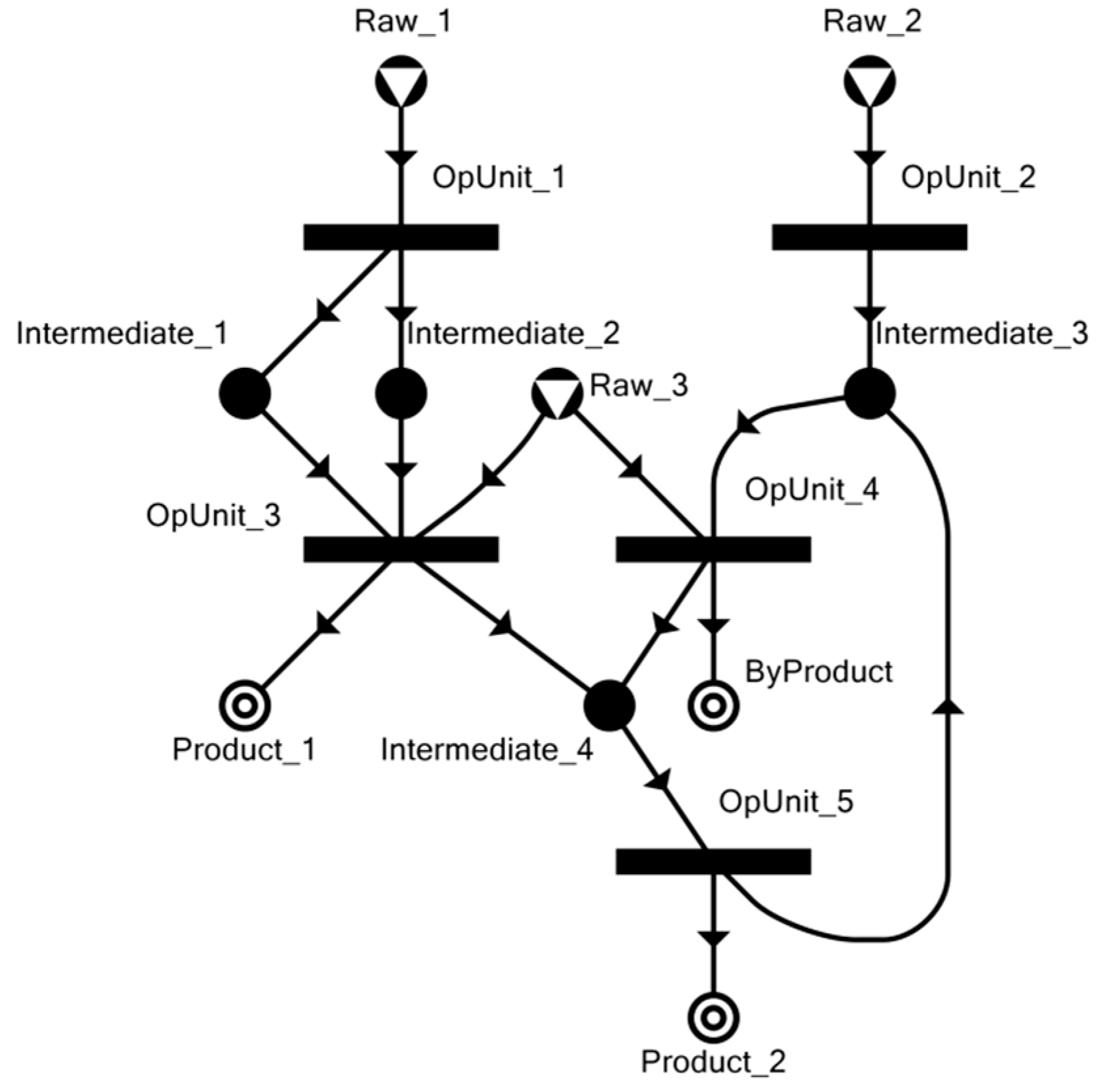
The P-Graph is a graph-theoretic model first introduced by Friedler et al. [9]. It is capable of modeling PNS problems unambiguously and gives options to effectively find optimal solutions. The model consists of a directed bipartite graph of a material node set and an operating unit node set. The material nodes resemble the states in the model. A state is usually representing the presence of some material or other physical or virtual property. The operating unit nodes represent transitions of a set of states into another. This is generally some kind of production step, transportation of goods, purchase, but may simply mean some logical consequence of the existence of a state based on others. Arcs from material nodes to operating unit nodes represent consumption. Arcs between operating units to materials represent production. That means the inputs and outputs of an operating unit are the materials for which there exist arcs going towards, and starting from the operating unit. In both cases, arcs are directed towards material flow. Materials can be both inputs and outputs at the same time. In this way, the P-Graph represents the structure of the process, see Figure 1. There are three types of materials in a P-Graph:
- Raw materials are the ones available from external sources, and cannot be produced.
- Final products are those we want to obtain.
- Intermediate material nodes are other materials involved in the system, typically in between the production chain from raw materials to final products. Intermediates can be produced by some operating units and can be consumed by others.
The goal of the PNS problem is to find a structure and operation for the system which is optimal in some manner. A structure of the system involves appropriate selection of available technologies and other activities, and the corresponding material flows. Optimality may refer to different objectives, typically it is cost minimization. A structure of the process network is to be found for which all products are obtained. This is called a solution structure, and it is, in general, a subset of the original P-Graph. Along with the rigorous mathematical definition of P-Graphs, five axioms are described that must hold for a P-Graph in order to be considered as a solution structure [9]:
- All of the final products of the PNS problem are represented in the resulting P-Graph.
- Any material has no input if and only if it is a raw material.
- Every operating unit in the P-graph is also defined in the PNS problem.
- Every operating unit is part of a path leading to a final product.
- Every material in the P-Graph must be the input to or an output from at least one operating unit in the graph.
The P-Graph framework also includes algorithms that can be used to solve PNS problems:
- The Maximal Structure Generation (MSG) is a polynomial-time algorithm which finds the so-called maximal structure of a PNS problem [10]. This structure is the union of all solution structures, and it is itself a solution structure as well, as a consequence of the axioms. The point in finding the maximal structure is that unnecessary parts of the PNS problem can be excluded a priori from optimization.
- The Solution Structure Generation (SSG) is an algorithm for systematically generating all solution structures of the PNS problem [11]. This is useful, because once the structure is fixed, other decisions like exact material flows are easier to determine. For large problems, the number of solution structures may explode.
- The Advanced Branch and Bound (ABB) method is an algorithm which finds the optimal solution of a PNS problem modeled as a P-Graph, driven by underlying MILP model constructed and decisions based on the combinatorial nature of the problem [12]. Note that MSG and SSG only operate on the graph itself, without other problem data like material flow ratios, costs, or capacities, see Figure 2.
These data also correspond to a PNS problem and the ABB is capable of presenting detailed solutions only when these are also available. PNS Studio is a software toll with which PNS problems can be designed as P-Graphs. These can also be solved using the SSG or ABB methods to find cost-optimal solutions for a process network. The software is freely available online [13], and was also used in the case study of this work.
2.2. Extensions of the P-Graph Framework
The P-Graph framework originally targeted chemical engineering problems, but the tool is useful for other areas as well. The framework itself was also extended by additional functionalities, either in implementation or application.
Time-Constrained PNS (TCPNS) is a problem where timing constraints on the flows can be added [14]. This gives the possibility to make scheduling decisions by P-Graphs. Note that this was already possible with the framework with certain circumstances. Certain vehicle routing problems where deliveries are fixed in time were also solved by P-Graphs before TCPNS was introduced [15]. Purely scheduling problems of process networks, where there is a fixed set of tasks and orders must be found with various storage policies, can also be addressed [16]. These methods most importantly show that operating units in P-Graphs do not necessarily resemble actual equipment, but possibly logical relationship, like conversion, or precedence relationships.
Separation Network Synthesis (SNS) is a production environment that can separate chemicals into their pure components in multiple possible ways that can be optimized. This is not a utility, but a production optimization problem, which can be transformed to a PNS problem and solved by the ABB algorithm [17].
In a PNS problem, the input and output ratios for operating units are fixed. This is not the case in some real world circumstances, when equipment units can have several different inputs with arbitrary ratios. Pelletizers and furnaces are an example for this. The model complicates if ratios are arbitrary, but also subject to constraints, like minimum or maximum ratios. The P-Graph framework was extended to address such case of input scenarios [18], as the underlying MILP model of the system was extended with linear constraints to obtain an appropriate model. Note that the P-Graph framework may be itself capable of modeling such operating units with several material nodes and operating unit nodes.
The P-Graph methodology can be extended to meet multi-periodic demands and supplies. Multi-periodic means different rates of production of final products or consumption of raw materials and products at various time periods, and optimization of the whole duration in a single model [19]. Periods are an important issue, because assuming average load during a period may lead to underestimating capacity needs during the year. This is especially true if operation should run at an extremely high rate in short periods, while at low rate in general, resulting in an average that is way under the capacity required to be operational at all times. However, the equipment units may have minimal required flow to be working, which complicates the operating unit model of the P-Graph, so the multi-periodic modeling scheme can possible be extended to model such technologies [20]. Although multi-periodic modeling is a logical extension of the P-Graph framework, which means it does not require additional tools to be implemented, the PNS Studio software already has support for making multi-periodic models easier [21]. Note that this usually requires manual addition of a vast amount of data, as each period is usually modeled by its own P-Graph, which is replicated. The PNS problem can get very difficult to understand if the number of periods is high.
2.3. Applications
The P-Graph framework can be applied to a wide range of process network optimization problems, including those for which production, utility, or transport systems are in question. The methodology is a useful alternative to implementation of Mixed-Integer Linear Programming models or other solution methods. For example, pinch analysis [22] is a widely used tool for system design, one possible application of which is energy sector planning with carbon emission constraints [23], but the same problem can also be solved by the utilization of P-Graphs [24]. Note that the ABB algorithm itself relies on linear programming. However, the P-Graph framework has some advantages, for example providing the series of the best solutions, in order, instead of finding just a single optimal solution [25].
A thorough collection of P-Graph applications can be found in [26], showing that the framework is useful in various case studies, including transportation, supply chain system design and plant management. There is a particular review that focuses on P-Graph applications on sustainability projects, like optimization from processing facilities to supply chains [27]. Another review is made by [28], which also notices possible future developments of the framework. Particularly, the theory allows more complex operating unit models than the current implementations can handle.
Polygeneration plant modeling can also be done by the P-Graph framework [29]. The recent study involves satisfying multiple uncertain demands like heating, electricity, cooling, and treated water. Not only the optimal, but the near-optimal solutions can be found. However, risks and possible reactions in case of equipment failure must be taken into account, which can also be handled by the same framework, as an alternative to linear programming models [30]. Uncertainty in supply and demand in general and risks for inoperability generally affects the usability of supply chains. The P-Graph framework was also used in such a scenario to analyze risks in the supply network of bioenergy parks [31]. A more simple case, in the modeling point of view, is when risks can be derived as parameters of the available technological options. This can be the case when probability of losses is attributed to each activity and these can be penalized in the objective [32]. The authors in the example seek to minimize fatalities in the whole bioenergy supply chain.
The framework was used to address a biomass supply chain enhancement [33], where P-Graphs and conventional mathematical programming tools were used simultaneously to obtain a decomposition of the main problem. The authors remark that the results must be regularly revised to reflect real circumstances. Several biomass types were considered in connection with the palm oil industry. Another set of biomass resources were inspected in a work of wood processing residues [34]. One drawback is observed in this case study, particularly, that minor changes to problem data may result in significant changes in the solution structures. This makes the option of finding near-optimal solutions valuable.
Addressing heat and electricity needs simultaneously is a common scenario for plant design. Available biomass is often considered in parallel or as a replacement with purchasing natural gas and electricity directly [35]. The case study, after optimization with the P-Graph framework, pointed out a potential 17% decrease in operating costs if biomass is integrated into the energy supply, while other objectives like ecological footprint can also be taken into account [36].
Spatial distribution of the biomass types and demands points can be simultaneously taken into account to address the optimization of a full renewable energy supply chain [37]. In their work, authors first determine clusters to minimize transportation needs by mathematical programming, and then apply a PNS model to optimize material flow in and between these clusters.
The methodology is also useful in determining bottlenecks in the complete supply chains for biomass utilization [38]. The proposed method also relied on the suboptimal solutions the P-Graph framework was able to find. The method was used to improve sustainability indices in three different, novel scenarios [39].
Synthesis of carbon management networks (CMN) is an important issue in the sustainability point of view, and lead to complex optimization problems. The P-Graph framework was used for the synthesis of biochar-based CMN [40]. The model uses a set of sources of biochar and a set of sinks, that are soils that can contain it, and operating units resemble transportation between sources and sinks. Note that in this case, the number of operating units is the product of the number of sources and sinks, and other limits, for example the contamination of the soils can also be taken into account. Another example for carbon management network optimization used P-Graphs in conjunction with Monte Carlo method [41]. The Monte Carlo simulation was used to test near-optimal solutions reported by the PNS solver, and estimate their robustness.
The multi-periodic modeling technique itself was first applied to a real world case study where corn production was investigated, for which the supplies and demands both change throughout the year [42]. In another model formulation, the method was used to optimize annual electricity production for various demands and sources. Afterwards, a polygeneration case study was performed that also addresses steam, chilled and treated water demands [43]. It can be seen that the multi-periodic scheme can be independently applied to the raw materials, or the final demands of a supply network, based on which of them are fluctuating.
3. Materials and Methods
In this section the P-Graph model to be solved in the case study is described in detail. Our previous work included the case study utilizing a single period model [44], and input data we use is also presented here. The present work has two major improvements. First, electricity and heating demands were modeled as a multi-periodic P-Graph model. Second, the modeling of some equipment units—namely, the pelletizer and the biogas plant—involves a technique that allows mass-based equipment capacities and flexible input of different kinds of biomass.
In the optimization problem, the energy supply needs of the manufacturing plant must be satisfied. This means that some investments are considered against the business as usual solution of purchasing all the electricity and heating power from the public service providers.
The optimization problem is modeled as a PNS problem. This requires that raw material, intermediate, and final product nodes, operating units and connecting arcs are defined. Moreover, problem data like raw material costs, available amounts, operating unit investment and operating costs and capacities, and energy conversion rules must also be explicitly defined. After determining the demands, the underlying single stage model is described. Afterwards, the way this model is extended into a multi-periodic one, is presented.
For the sake of simplicity of the model, all energy quantities are expressed in kWh, regardless of being heat or electricity at a particular point in the process network. Monetary quantities are expressed in HUF. The value of this currency had been fluctuating, one EUR was between 300–330 HUF in the recent years where data into the case study were collected from. In the scenario for the manufacturing plant, expenses were in HUF uniformly. It shall be noted that interpreting results with an exchange rate to another currency only involves a linear factor for all monetary values, including the minimized total costs, but the obtained solution structures and their order would remain the same.
3.1. Electricity and Heating Requirements
The plant has two needs that are subject to the scenario: electricity and heating. These are the demands in the process system, and are modeled as product nodes in the resulting P-Graph. The business as usual solution is that electricity is bought from the grid in the amount needed. Heating is provided by the plant’s own furnace, in which natural gas is fed, bought from the public service provider.
Detailed consumption data about the plant’s natural gas consumption was provided in Table 1. The plant requires indoors heating. The heating requirements are therefore modeled as the total heating value of gas or other materials and energy consumed, with possible conversion ratios depending on source. A single yearly heat consumption value is assumed to describe the requirement. We can see there are significant fluctuations from year to year, with a clear tendency of decreasing, which is probably due to the company optimizing its operation constantly. Also, the heating requirements are a magnitude larger at winter than at other times of the year. This is the key fact that motivated the multi-periodic modeling scheme to be applied in this case study.
Electricity consumption data was also provided in a similar manner (see Table 2).
Electricity consumption also shows a decreasing tendency, but the consumption rates do not seem to clearly depend on the month. They more likely depend on production load of the plant, or other causes for which are unavailable in this case study. It can also be seen that the decreasing tendency is not necessarily rigorous: in the last year with known data, 2014, electricity consumption actually increased. For these reasons, the following decisions were made about the modeling method of the demands:
- Future demands that are used in the model are estimated based on a recursive formula of the data shown.
- Two periods are introduced to be handled differently: winter (from December to February, inclusive), and the other part of the year (from March to November, inclusive). From now on, we call these winter and mid-year periods.
The formula we used in the case study for demands were the following. This is applied to both the natural gas and the electricity consumption:
The first three years are omitted, since the significantly larger consumption in those is due to past changes in the plant operation. For the last three years, we apply a weighted average, with weights of 0.8, 0.9 and 1.0 for 2012, 2013 and 2014, respectively (note that 0.8 + 0.9 + 1.0 = 2.7). It is multiplied by a factor of 1.15 for more security of the energy supply, and to accommodate a slight potential increase.
This single value, obtained for both the electricity and heat demands, are used assuming them to be the constant yearly demands in all consecutive years. Nevertheless, it shall be noted that this is a rough estimation. Actual data could severely affect the results provided by our model. However, the P-Graph model we present can easily be resolved with different data.
To be able to model a multi-periodic scenario, the demands must be estimated for each period individually. Note that even though electricity consumption is somewhat independent of the periods, we have to calculate periodical demands since heat and electricity production can both be done from the same energy sources. The electricity and heating demands we suppose in the case study are summarized in Table 3. Note that it is obtained as a direct application of Equation (1) on data from Table 1 and Table 2.
In the P-Graph model, the four periodical demands represent the final product nodes. They must be satisfied with a combination of the available technologies, which are able to produce heat, electricity, or both.
3.2. Energy Sources and Their Availability
In the previous section, the final products of the process network were defined. Now, the raw materials are introduced. In the present case study, there are different kinds of energy sources considered. In general, there are more options, but due to the properties and environment of the plant, the following resources were included:
- Public service providers, from which unlimited amount of electricity and natural gas can be purchased.
- Solar power, which is also unlimited, as long as there is solar power plant capacity.
- Several different kinds of biomass of limited availability from the same region.
For purchased electricity and natural gas, and the different kinds of biomass, we assume a unit cost for each resource. Purchased electricity and natural gas are unlimited sources. This means that practically any amount can be purchased as long as the company is willing to spend the money needed. Solar power is freely available. Of course, it does not mean that solar power is a free energy source. Rather, regardless of the amount of solar power plant capacity we want to invest into, there is always a supply of solar radiation. The different kinds of available biomass are purchased locally. Note that these have a limited availability, as these are mostly byproducts from agriculture. Biomass has a drawback of having low energy content. Transportation of biomass over longer distances is not economical, and does not have a sense in the sustainability point of view either. We assume that the biomass types each have an own fixed unit cost, and an upper limit for purchase.
The energy sources are represented in raw material nodes in the P-Graph. Table 4 contains data for these raw materials. We must note that these are estimations we assume in this case study. We also assume that there is no concurrent demand for these materials from other parties. Each of the enlisted raw materials corresponds to a raw material node in the resulting P-Graph.
Note that there are costs associated with the processing of these resources. These are embedded into the operating costs of the operating units instead. For example, maintenance costs of the solar power plants are costs of the power plant, not the solar energy itself. The reason behind this scheme of modeling is that raw material nodes can have a straightforward implementation in the P-Graph based on the unit prices and available amounts.
3.3. Operating Units
In a P-Graph, all transformations of materials to others are done by operating units. This means that an operating unit may resemble an actual technological step, or market operations like purchase or selling, or only be a modeling tool. In this case study, operating units are introduced to fit into the following roles:
- Direct supply by purchase of electricity or natural gas.
- Solar power plants.
- Biomass processing chain.
Note that these roles are in a one-to-one correspondence with energy source types. Those operating units that correspond to actual equipment units that require investment and operating costs are shown in Table 5, with the following meanings:
- Fixed investment costs are to be paid once, at investment, if the technology is used.
- Proportional investment costs are to be paid once, at investment. The amount is proportional to the yearly capacity of the operating unit, which cannot be changed later.
- Fixed operating costs are paid yearly, for using the operating unit, regardless of rate of utilization.
- Proportional operating costs are paid yearly, for using the operating unit, and are proportional to the actual utilization of the operating unit.
This means we assume that each possible investment has linear costs in terms of capacity, with a starting fixed investment cost. This assumption is required in order for the network to be modeled with the P-Graph framework. More complex cost functions can be estimated, or alternatively, different operating units can be introduced in the model if necessary. Investment costs appear as costs evenly distributed in the investment horizon. That means if a longer horizon is considered, then investment costs are decreasing in the modeling point of view, as the current model seeks to minimize yearly operating costs.
Note that the P-Graph methodology would allow the modeling of any operating units which can operate in parallel to each other from the modeling point of view, as long as they can be properly represented by linear fixed and proportional investment and operating costs and capacities. In this case study, some technologies like heat pumps were initially excluded by the management due to the plant’s properties, electricity needs, initial investment costs, and lack of subsidized project possibilities.
Other operating units in the process network are either already present or only represent some activities that are not physical production steps. This means that other operating units have neither investment nor operating costs, nor maximal yearly capacities. We assume that all operating requirements can be expressed in the aforementioned costs, including energy requirements. Note that, for safety reasons, the plant would anyways be connected to the grid. This makes any particular solution easily adjustable if demands unexpectedly increase. It also means that the possibility of self-sustaining energy supply is neglected in this case study.
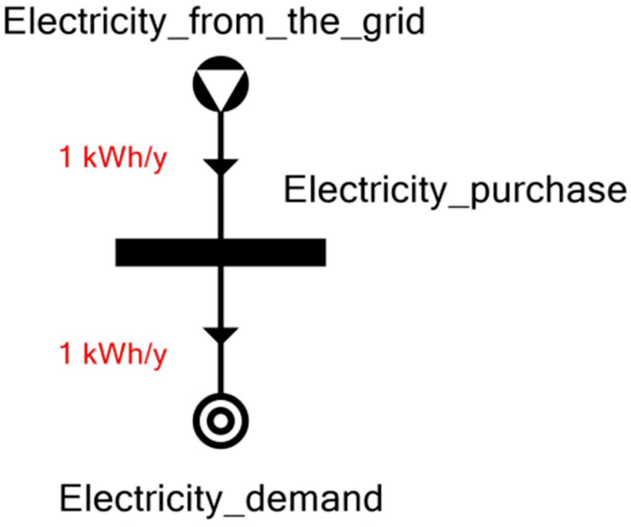
3.4. Direct Purchase
The electricity consumption is the simplest operation in the process network. An operating unit representing electricity purchase from the grid is introduced. Its single input is the electricity from the grid, and its single output is the electricity demand as depicted in Figure 3.
The natural gas purchase is done by a single operating unit. This unit has a single input and output: natural gas from the provider, and purchased amount. In contrast to electricity, natural gas purchase is not directly supplying heat. For this reason, the manufacturing plant has a furnace which consumes the natural gas purchased, and produces the heat demand. Transfer ratios represent the heating value of natural gas, which is 34 MJ per m3, converted to kWh as shown in Figure 4.
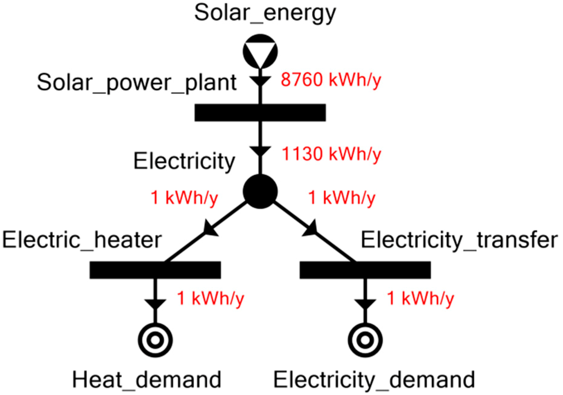
Solar power is considered as an alternative energy source to be exploited solely by solar cells. This means that a solar power plant is introduced which transforms solar power into electricity. By estimation, we assume that 8760 kWh solar energy can be converted into 1130 kWh of electricity, or any amounts with this same ratio. Note that although the efficiency of solar cells is important in reality, only the output of 1130 kWh is of interest in this model. The reason for this is that solar energy is free and unlimited anyways, and solar power plant investment and operating costs are given in terms of throughput, see later.
The reason for using the number 1130 kWh is that the proportional investment and operating costs were originally available as 400,000 HUF and 25,000 HUF per 1130 kWh/y throughput (see Table 5).
The electricity produced by the solar power plant can be directly fed into the electricity demand. Alternatively, an electric heater can be utilized, which contributes to the heat demand, see Figure 5.
3.5. Biomass Utilization
The biomass supply is a bit more complicated. First, some kinds of the biomass are needed to be pelletized first. Table 6 summarizes the data for these materials, which are sawdust, wood chips, sunflower stems and vine stems. Note that different pellets have slightly different energy contents. This fact is a key observation for correctly modeling the pelletizer.
Pellets and the rest of the biomass, see Table 7, are considered as feeds into a biogas plant. Note that the heating value of each input type determines the amount of heating power the resulting biogas has.
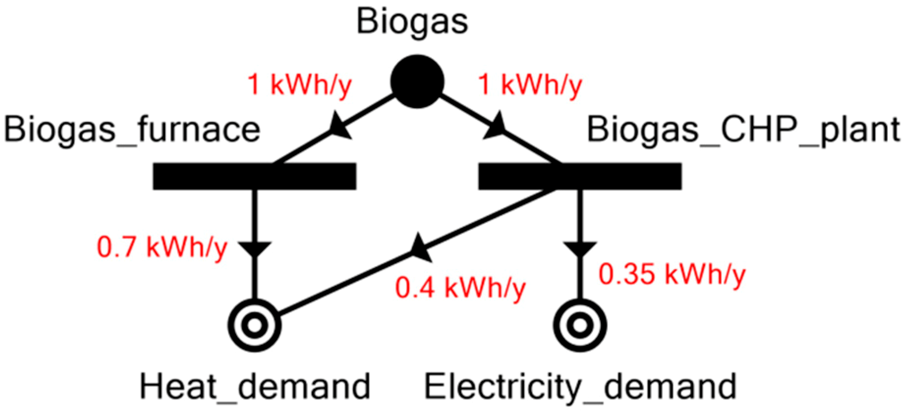
The biogas can be fed into either a biogas furnace, or a biogas-based “Combined Heat and Power” (CHP) plant. The former generates heating only, while the latter also produces electricity. We model these operating units in the following way, see Figure 6:
- The input of each operating unit is the total energy content of the biogas available. This is a single material node.
- The biogas furnace consumes 1 unit of biogas, and produces 0.7 kWh heating power, or different amounts with the same conversion rate.
- The biogas CHP plant consumes 1 unit of biogas, and produces 0.4 kWh heating power and simultaneously 0.35 kWh electricity, or different amounts with the same conversion rate.
- Productions are directly fed into the demands of the process network.
Attention is required to correctly model the part of the network from the biomass inputs to the biogas heating power. The key observation is that different inputs yield different energy contents. One way this can be modeled, used in [44], is the following procedure:
- Define a common input material node for both the pelletizer and the biogas plant.
- For all actual inputs, introduce a logical operating unit in the model which transforms the input to its heating power, which is a linear transformation. These are fed into the inputs of the equipment.
- From now on, the operating unit of the pelletizer and the biogas plant consumes the material introduced for the heating power of its inputs, and not their mass.
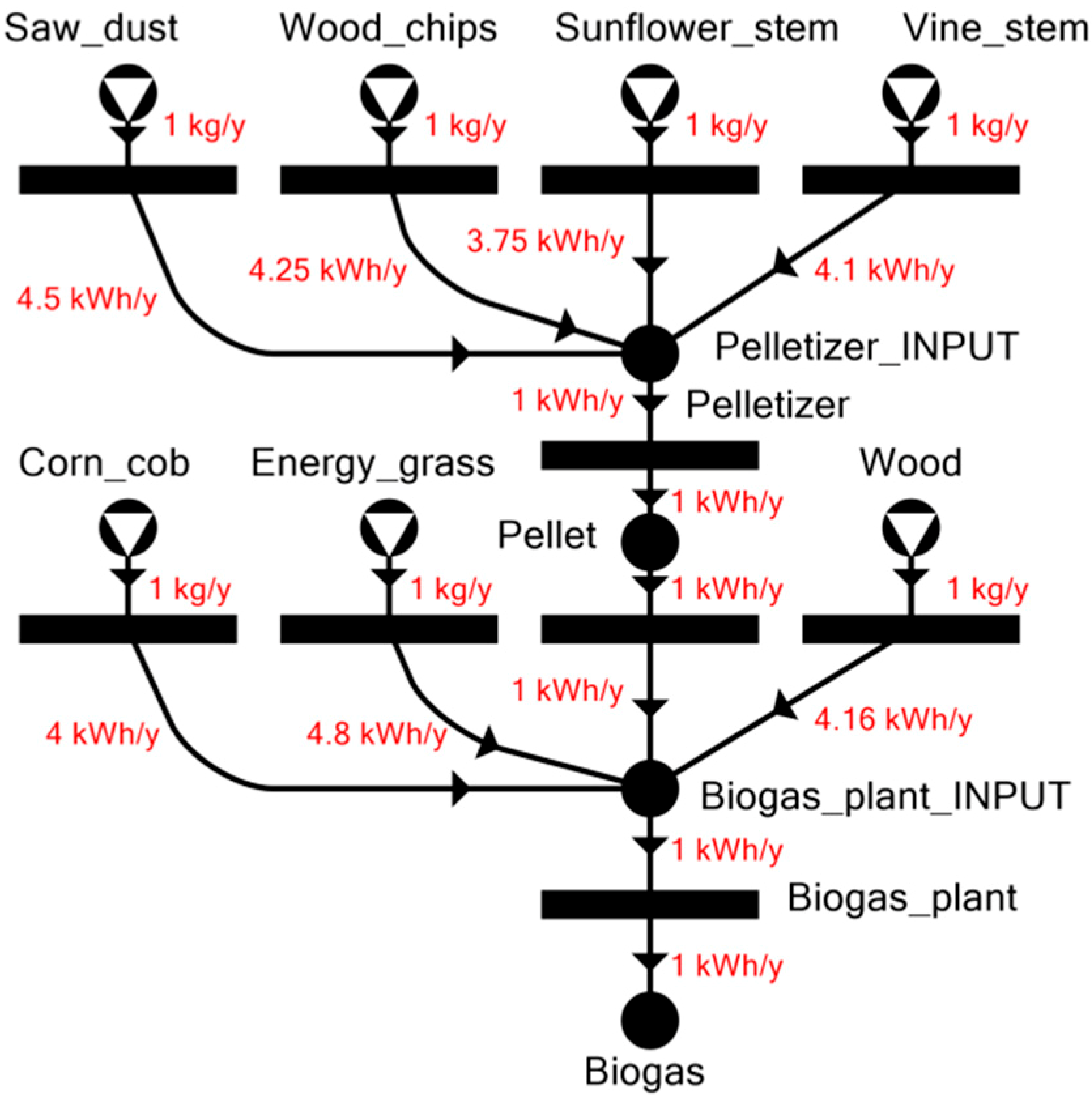
In this way, the heating content of each individual biomass type is respected and properly transferred until the heating power of the resulting biogas. The P-Graph resulting from this approach is depicted in Figure 7. Note that the appropriate point for modeling energy losses is the conversion factors in this design, so it is not happening at the pelletizer and biogas plant operating units in the model.
3.6. Modeling of Capacity Restrictions and Flexible Input Ratios
The problem with this approach is that the pelletizer and the biogas plant have capacity restrictions based on the mass of their inputs, not their heating power. It is natural, as a pelletizer does not “know” anything about the heating power of its product, only the mass. We must note that the original approach is therefore a modeling simplification which does not introduce a large error on the network, for two reasons. One is that operating costs for the pelletizer and the biogas plant are negligible compared to other terms like material costs and power plant investments. The second reason is that the conversion ratios for all kinds of biomass are similar in magnitude. To correctly model these operating units, a different approach is used in the present case study, summarized as follows:
- An individual logical operating unit is introduced for both the pelletizer and the biogas plant, which represent the investment, have no inputs, and produce a “production capacity” material. This is a logical material that can be distributed among the possible inputs arbitrarily.
- For each input, its pelletizing and biogas production operation is modeled by an individual operating unit each. These consume the production capacity from the corresponding investment.
- The four pelletizing processes produce different materials, for the different pellet types, in a ratio of 1:1 compared to input.
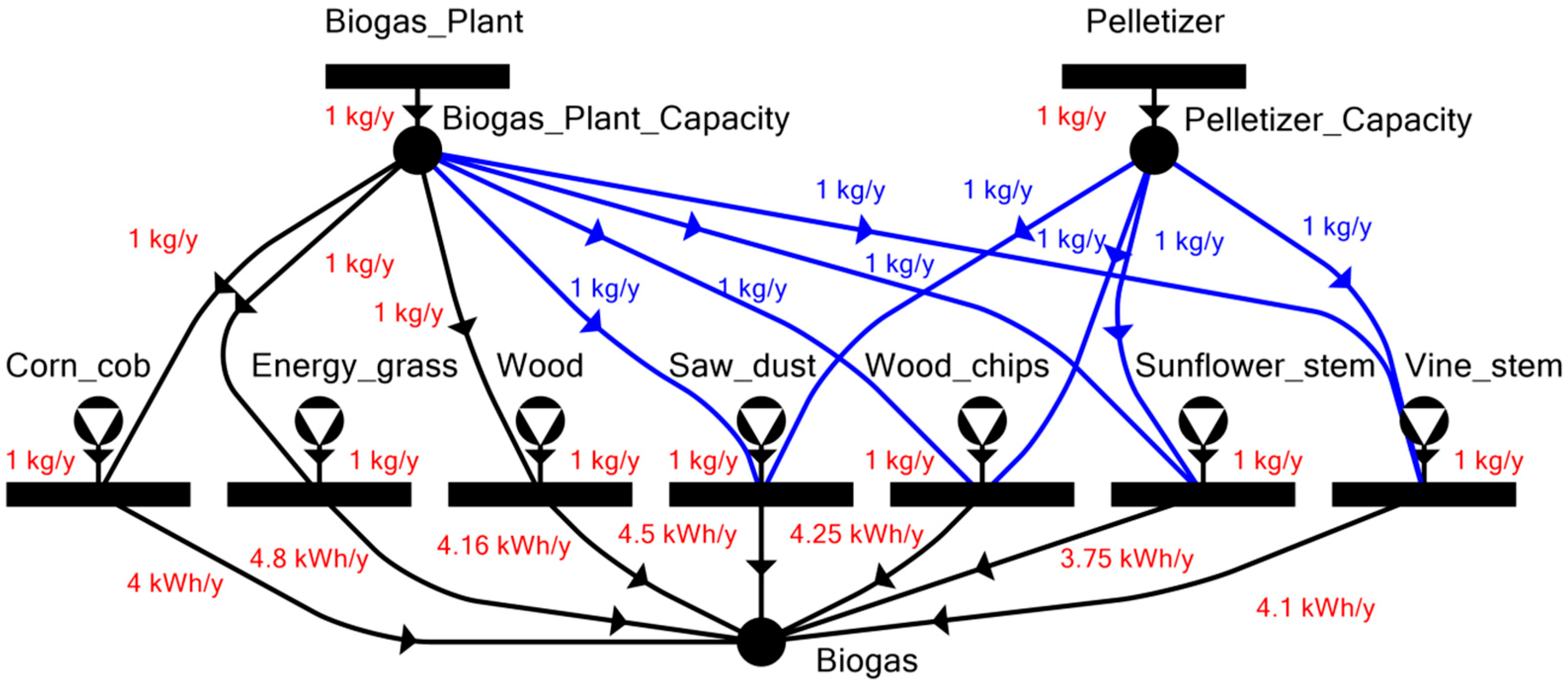
In this way, the heating values of the different biomass types are respected in the model, and the pelletizer and biogas plant is constrained by their actual total utilization rates, expressed in total mass of inputs. This approach can be summarized in Figure 8.
Note that simplifications can be made in this design. Observe that pellets have no other usage in the process network than being fed into the biogas plant. This way, the logical operating units of the pelletizer and corresponding ones of the biogas plant can be merged. This means that the pelletizer and the biogas plant together have seven logical operating units that produce the biogas. Each logical operating unit is corresponding to a biomass input type. The final form of the biomass supply part of the P-Graph model is depicted in Figure 9. Energy conversion ratios do not only reflect the heating values of the raw materials, but also the possible losses until the final conversion to heating power.
3.7. Multi-Periodic Model
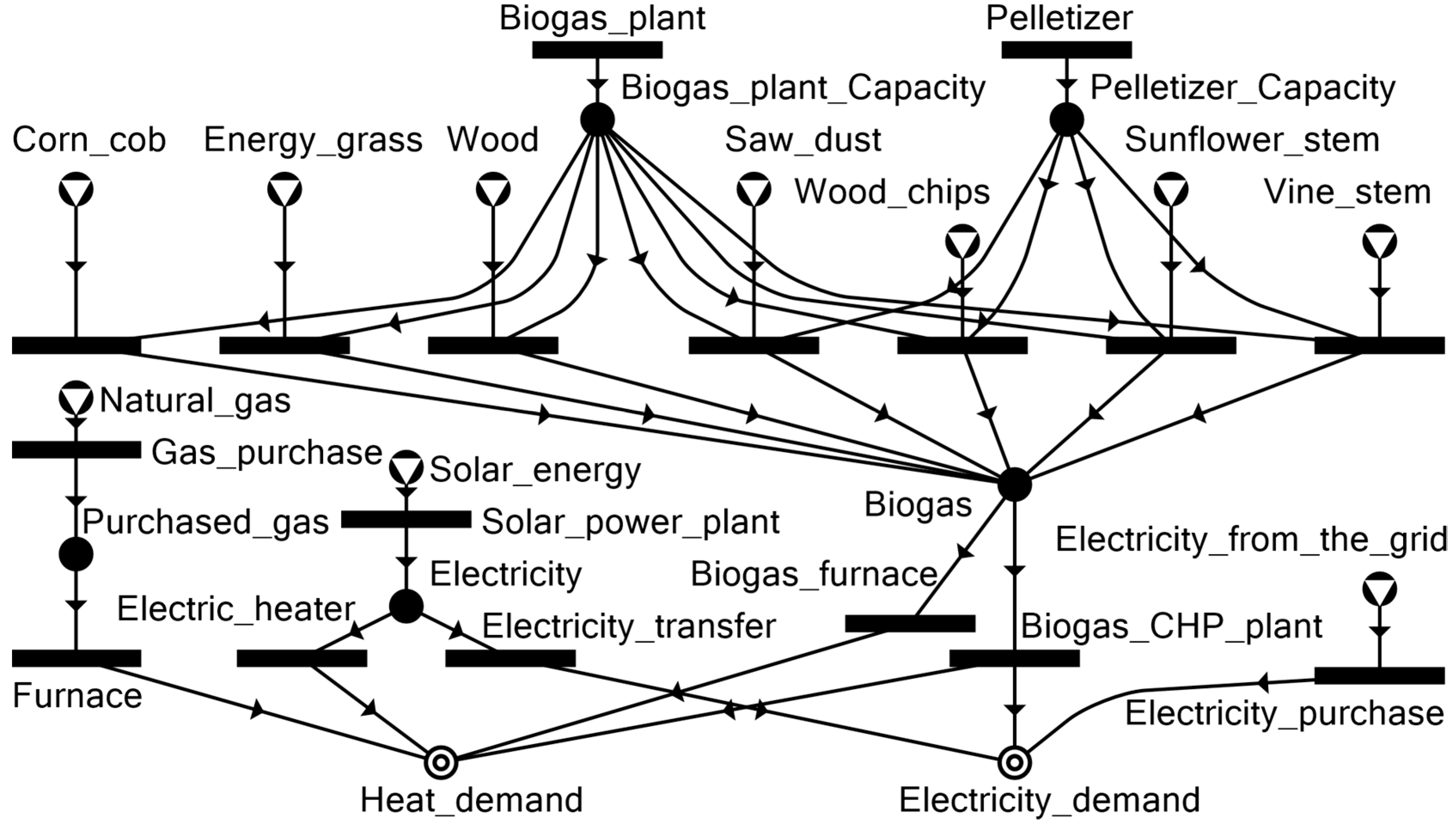
So far, the constructed P-Graph of a process network only considers a single period of operation. In a single period model, all data are given on a yearly basis—that means yearly total demands, and yearly total production rates. It is generally assumed in this case that timing of the production can be arranged to fit the demands arising throughout the period. This can be a valid assumption in some cases. One case is when there are little fluctuations in the supply and the demand, so a constant rate of production and demand satisfaction can be assumed in the whole period. Another case is when there is storage available for the production, and that is used up on demand. The single period P-Graph model is depicted in Figure 10.
Into this model, we introduced two different periods instead of the single period of one year. The nine months long mid-year and the three months long winter period are used. Each period has its own demand that must be satisfied. For example, heating demands are considerably higher during winter than at mid-year (see Table 3).
We assume that demands are fixed to the periods, but supplies are not. The required heat must be produced or purchased in the period where it is demanded, and no energy transfer is possible between periods. On the other hand, the same yearly supply of each limited raw material (biomass) is available throughout the year, and can be used up in the periods in any ratios and combinations. This implies that storage from one period to the next is assumed to be available, and its requirements are neglected. Note that the multi-periodic modeling technique would allow binding the supplies to the periods, and also properly modeling significant storage costs and capacities.
Solar energy works a bit differently than raw biomass, because throughput is generally much lower at winter than at mid-year. This is a significant factor that is addressed in the model. Concluding the multi-periodic scheme, demands are calculated for each of the two periods, while supplies are freely distributed between periods—the only exception being the solar radiation.
The data we use about solar power plants is that a production of each yearly 1 kWh of electricity requires 353.98 HUF proportional investment and 22.12 HUF proportional operating costs. These are distributed across a 3 months long winter and a 9 months long mid-year period. If an investment is made, we assume that the solar power plant is utilized throughout the year. For this reason, there is no point in dividing the costs of the plant between the periods. What actually makes sense, is dividing the throughput between the periods. We assume that, on average, solar power plants are times more efficient in mid-year, than in winter. Provided that a total yearly production of electricity is given, we can calculate the amounts and from the following formulas:
This means that, in the multi-periodic model we assume that a production of kWh electricity at winter and kWh production at mid-year requires an investment cost of 353.98 HUF and a yearly operating cost of 22.12 HUF. These are both proportional costs.
The way we transform the single period P-Graph model into a multi-periodic one with the aforementioned two periods, is the following:
- The P-Graph is duplicated, each having the same set of raw materials, intermediates, final products, and operating units. One clone is for each period.
- The raw materials are merged between periods, as they are available for consumption at any time.
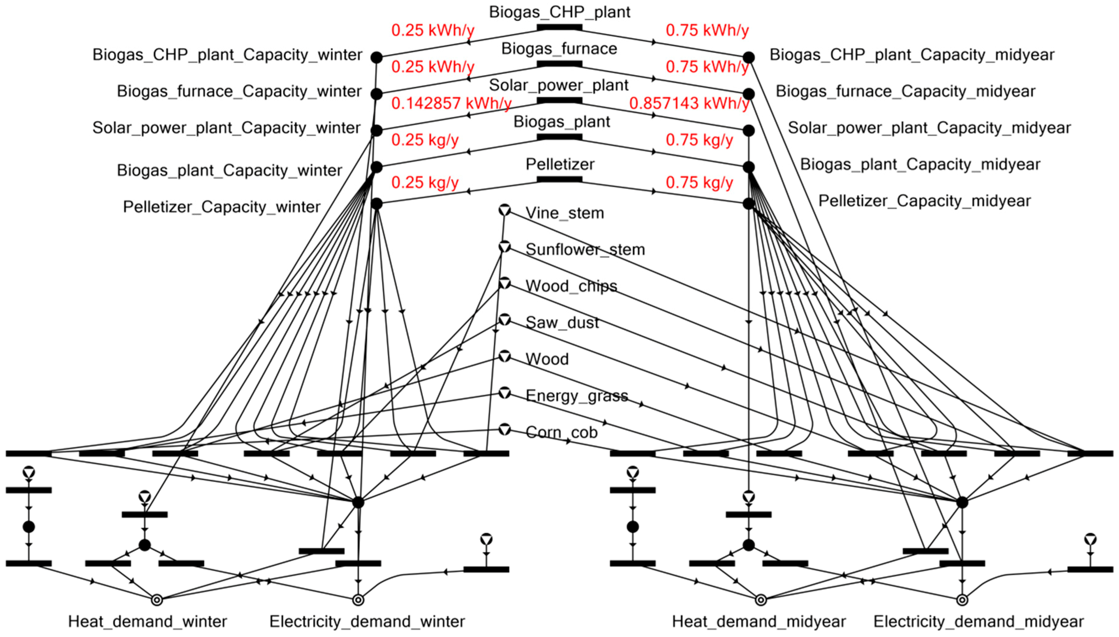
- The operating units for the biogas plant and the pelletizer, which hold the cost data of these two equipment units, are merged for each, while keeping both of their capacity outputs. The new operating units produce the logical “production capacity” materials in a ratio of for winter, and for mid-year, because of the respective lengths of the periods. These capacities can be freely used in each period, by each of the available logical operating units representing pelletizing and biogas production from a particular input.
- For the biogas furnace, biogas CHP plant and the solar power plant, we replicate the scheme applied to the biogas plant and the pelletizer. A single operating unit is introduced holding the cost data, which produces two logical “production capacity” materials—one used in winter, one used in mid-year. The ratio of capacity generation is for winter and for mid-year, with the exception of the solar power plant, which produces for winter and for mid-year. The production capacity materials are consumed by the only logical operating unit in the period, representing actual production.
- For the rest of the operating units, like the electricity transfer, electric heaters, natural gas furnace, the duplicates remain, as there are no costs or other constraints associated with these operations that would require to be treated globally for the two periods.
The resulting final multi-periodic P-Graph model is shown in Figure 11. We can observe that the same scheme is applied to the five operating units with costs. This scheme had been already done halfway for the pelletizer and the biogas plant, not because of the multi-periodic model, but for the sake of modeling the capacities correctly.
4. Results and Discussion
The single period and multi-periodic models were solved by the PNS Studio program, version 5.2.3.1, on a Lenovo Y50-70 laptop computer equipped with an i7-4710 HQ processor and 8 GB RAM. Note that the problem sizes are relatively small, which means that solution should be fast on any modern computer. First, both models were solved with an assumed investment horizon of 20 years. Then, lower horizons were set. We could observe that the MSG algorithm reports the P-Graphs themselves as maximal structures. The reason behind this is that these P-Graph models do not contain any redundancy. All parts are candidates for an optimal solution. The ABB algorithm was launched, and the first few best solution structures were manually investigated. The algorithm succeeded in 1 s for the single period case, and 2 s for the multi-periodic case. The P-Graph model files for PNS Studio and solutions discussed here are available in the supplementary materials.
4.1. Single Period Model
The optimal solution is 220.709 M HUF/y operating cost for the single period case. The 10 best solution structures (including the first, optimal) are summarized in Table 8. Note that the usage of the Pelletizer and the Biogas plant are a direct consequence of the existence of their respective raw materials in the model. We can see that the first few solution structures differ only slightly in terms of the yearly cost. The difference between the #1 and #10 solutions is 2.72%. Still, a unique set of energy sources is used each time. This means that all of these solutions can be sensible choices, as little change to the data, or other factors considered may justify the selection of an alternative of the optimal solution.
The biogas CHP plant is used in all cases, making it a very useful candidate for sustainable energy supply. Contrary, the biogas furnace is not present in the first few solutions, even though it is cheaper. This means that the greatest advantage of the biogas CHP plant is that it can generate electricity. Note that also all seven types of biomass appear in different combinations. Decisions on which is the better and worse are determined by their available amounts, costs and heating values, and whether they must be pelletized or not.
We shall also note that even though solar power plants appear in solution structure #9, it is only used for electricity production. Purchase of natural gas or electricity from the grid is still present in many solutions. Actually, #9 is the only one where purchasing electricity is completely eliminated. There are structures where both additional heating and electricity is required from the providers.
It may be an important question whether the resulting solution structures actually represent good practical choices. One security concern is that if the manufacturing plant is only relying on its own energy supplies, then unforeseen shortages could lead to vast losses. This is not a high risk in our model. In the worst case, electricity and natural gas can still be purchased, even when the scenario is set to completely omit these sources. These options are valid because no investment or operational costs are required for purchase, and the manufacturing plant already has a furnace. If we assume this infrastructure is maintained, losses can be kept minimal.
4.2. Multi-Periodic Model
The optimal solution for the multi-periodic model is 228.942 M HUF/y, see Figure 12. The used options for the 10 best solution structures again are listed in Table 9. The optimal solution for the problem utilizes the biogas plant and a biogas CHP plant for producing part of the requirements at mid-year and at winter. Note that energy grass and corn cobs are utilized at full capacity of the purchased equipment units. Energy grass is the dominant biomass supply, but direct purchase of energy is also needed. It is also worth noting that each period can have an individual supply. In this example, natural gas purchase is not needed at all mid-year, but is utilized at winter. Resource utilization of this solution is detailed in Table 10, and plant capacities in Table 11.
Several interesting facts can be deduced from the solutions. First, the objective for the multi-periodic model is slightly worse than the objective for the single period case, by 3.73% at the best structures. This is natural, because the multi-periodic is a more accurate model with additional requirements. This means that not only the total demands must be satisfied, but the demands for each period individually, which is a more restrictive condition.
We can also see that solution structures show little variation, either in structure, or in objective values. Solution #1 and #10 have a difference of just 0.2%. The reason behind this might be that multi-periodic models have much more solution structures in general than their single period counterparts. We suspect that the technologies and options observed in the single period case would turn up if more solution structures of the multi-periodic model were investigated.
The general structure of the first few solutions is that the biogas CHP plant is used as the only investment. It is sufficient to serve the heating requirements in the mid-year period, but natural gas purchase is always required in the winter period. In both periods, the electricity requirements are still not satisfied, so electricity must be purchased. The solar power plant does not appear in the first few solutions. This might be due to the fact that it is especially weak in the winter period. Saw dust and wood chips do not appear in the first 10 solutions, while energy grass is used in all cases, in both periods. There are very small differences between some structures. For example, #1, #2 and #3 only differs on the fact that whether corn cobs are used in winter, mid-year, or both.
Overall, we can observe how the multi-periodic models behave compared to their single period counterparts. The case is more restricted, but there is also more flexibility. The energy supply scenario can be different for the winter period and the mid-year period, even though exactly the same investments are available in both.
4.3. Shorter Investment Horizons
The costs of units in the model have two components, operational cost and investment cost. The investment horizon is used to annualize the investment cost. The horizon in this model means the length in years for which the annually most profitable solution is to be found. Consequently, the investment costs are divided evenly in the investment horizon. Note that this is different from the payback time of a single operating unit, as the investment horizon is a single parameter for the optimization of the whole system. The purchased equipment units are assumed to be in their useful life throughout the horizon, but management often considers only those solution scenarios which are profitable in a much shorter term. As yearly investment costs are vast and are depending on the horizon length, this modeling parameter should be investigated.
The former investigation was done assuming a 20 y horizon, now additional results for shorter ones, 10 y and 5 y are presented. The first two solution structures for each model and in each considered horizon length are shown in Table 12.
What can be seen is that even for 10 y, the business as usual solution is the optimal. This means that all heating and electricity demands are purchased as natural gas and electricity from the grid, rather than being produced, and no additional investments are made. This exact solution is actually the optimum for both the single and multi-periodic cases, for both 10 y and 5 y of investment horizons. It may happen that the two different models, the single and multi-periodic ones, have a common solution, as in this case.
Note that the best solution for 20 y horizon in the multi-periodic model is the same as the second best for the 10 y horizon case. The second best solutions for 10 y horizon in both models are technically the same. Corn cobs and energy grass are used in a biogas CHP plant. These solutions have a considerable difference from the optimal business as usual solutions, 6.15% at the single period model, and 4.71% at the multi-periodic model. These are larger differences than can be observed in the first 10 solutions of the 20 y horizon cases.
For the 5 y horizon, the situation is much worse; there is a whopping difference of 35.7% for the single period case, and 28.27% for the multi-periodic case. Note that the second best solutions for both models are technically similar. This time, the so far ignored biogas furnace is the option, supported by energy grass consumption. The reason behind this is that probably the biogas furnace is the cheapest working investment, if we want to invest into something and leave the business as usual solution at all costs.
One interesting thing is that the seemingly more restrictive multi-periodic model has a better second best solution than its single period counterpart in the 10 y and 5 y investment horizon cases. The reason for this is that in the multi-periodic solution, gas purchase helps, but only in winter. This is not a possible option in the single period case.
These results have shown that the biomass and solar power availability are not so promising in this particular case study, because these investments would require a long time to become economical. Companies usually plan for much shorter time horizons. However, the situation is constantly changing, better technologies may appear, or more endorsement for sustainable energy supplies. The P-Graph model can be easily adjusted if a scenario with different data and other technologies are introduced, provided that similar assumptions can be made as in this work.
5. Conclusions
A P-Graph model was developed, and the energy supply options of a manufacturing plant in Hungary were investigated. The general PNS was defined, and the P-Graph framework was introduced. Step by step, the P-Graph model of the problem was constructed. Estimates on future demands were made to serve as a basis for our optimization model. We defined the raw materials, the demands, the intermediates, and the operating units. Parameters were gathered to materials and the operating units but the structure of the model has the main focus. Modeling techniques were presented for the P-Graph framework to handle situations like mass-based capacity limitations, multiple potential inputs with arbitrary ratios or activities like purchasing. A multi-periodic P-Graph is implemented which differentiates winter and mid-year consumption. It is capable of modeling operating unit capacities when demands are fluctuating, and also takes into account solar energy supplies.
The PNS Studio software was used to solve the single and multi-periodic models with the ABB algorithm. The multi-periodic scenarios establish that energy supply methods can vary between winter and other parts of the years. It can be observed from the results that significant improvement can be obtained compared to the business as usual solution, where all electricity and heat is purchased from the market. However, this requires that the investments of local energy supply options, biomass and solar energy utilization have a long investment horizon. This means that although there are considerable options for sustainable energy supplies, as they are beneficial in the long-term, the economical environment significantly impacts their efficiency.
The P-Graph model was shown to be capable of determining the best solutions for an energy supply optimization problem. Note that other aspects can be included in the future. Upgrades like insulation, better heating system, energy saving light bulbs, and other investments can be incorporated to yield a more precise model for the demands, as well as other power plant types and resources. Storage and exact availability of raw materials can still be modeled in a multi-periodic manner. Other demands, like the water system of the plant can be governed by a single unified PNS problem. Nevertheless, the current model is capable of handling similar supply and investment options with different data, with minor modifications.
Supplementary Materials
The following are available online at https://www.mdpi.com/1996-1073/12/8/1484/s1. The P-Graph model files for the case study presented, in PGSX format, with a few solution structures. These can be viewed, edited or resolved by the P-Graph Studio software. Images of the solution structures from the mentioned cases are also provided.
Author Contributions
Introduction, I.H. and H.C.; Materials and Methods, A.É. and I.H. Results, A.É. and H.C.; Discussions, A.É.; Conclusions, I.H. and L.H. Review and editing, H.C. and I.H. Solver programming, L.H.
Funding
We acknowledge the financial support of Széchenyi 2020 under the EFOP-3.6.1-16-2016-00015.
Acknowledgments
We gratefully thank Adrián Szlama for his work on the P-Graph model and data collection and evaluation.
Conflicts of Interest
The authors declare no conflict of interest.
References
- US Census Bureau. US and World Population Clock. Available online: www.census.gov/popclock (accessed on 16 March 2018).
- Worldwatch Institute. The State of Consumption Today. Available online: www.worldwatch.org/node/810 (accessed on 16 March 2018).
- Running, S.W. A Measurable Planetary Boundary for the Biosphere. Science 2012, 337, 1458–1459. [Google Scholar] [CrossRef] [PubMed]
- US Energy Information Administration. First Use of Energy for All Purposes (Fuel and Nonfuel). Available online: www.eia.gov/consumption/manufacturing/data/2010/pdf/Table1_1.pdf (accessed on 16 March 2018).
- International Energy Agency. Electricity Statistics. Available online: https://www.iea.org/statistics/electricity/ (accessed on 20 February 2019).
- Saavedra, M.R.; Fontes, C.H.O.; Freires, F.G.M. Sustainable and renewable energy supply chain: A system dynamics overview. Renew. Sustain. Energy Rev. 2018, 82, 247–259. [Google Scholar] [CrossRef]
- Nemet, A.; Klemeš, J.J.; Duić, N.; Yan, J. Improving sustainability development in energy planning and optimisation. Appl. Energy 2016, 184, 1241–1245. [Google Scholar] [CrossRef]
- Kalaitzidou, M.A.; Georgiadis, M.C.; Kopanos, G.M. A General Representation for the Modeling of Energy Supply Chains. Comput. Aided Chem. Eng. 2016, 38, 781–786. [Google Scholar]
- Friedler, F.; Tarjan, K.; Huang, Y.W.; Fan, L.T. Graph-Theoretic Approach to Process Synthesis: Axioms and Theorems. Chem. Eng. Sci. 1992, 47, 1973–1988. [Google Scholar] [CrossRef]
- Friedler, F.; Tarjan, K.; Huang, Y.W.; Fan, L.T. Graph-Theoretic Approach to Process Synthesis: Polynomial Algorithm for the Maximal Structure Generation. Comput. Chem. Eng. 1993, 17, 929–942. [Google Scholar] [CrossRef]
- Friedler, F.; Varga, B.J.; Fan, L.T. Decision-Mapping: A tool for consistent and complete decisions in process synthesis. Chem. Eng. Sci. 1995, 50, 1755–1768. [Google Scholar] [CrossRef]
- Friedler, F.; Varga, B.J.; Fehér, E.; Fan, L.T. Combinatorially Accelerated Branch-and-Bound Method for Solving the MIP Model of Process Network Synthesis. In State of the Art in Global Optimization; Floudas, C.A., Pardalos, P.M., Eds.; Kluwer Academic Publishers: Dordrecht, The Netherlands, 1996; pp. 609–626. [Google Scholar]
- P-Graph Studio. Available online: http://pgraph.org (accessed on 31 January 2019).
- Kalauz, K.; Süle, Z.; Bertok, B.; Friedler, F.; Fan, L.T. Extending Process-Network Synthesis Algorithms with Time Bounds for Supply Network Design. Chem. Eng. Trans. 2012, 29, 259–264. [Google Scholar]
- Barany, M.; Bertok, B.; Kovacs, Z.; Friedler, F.; Fan, L.T. Solving vehicle assignment problems by process-network synthesis to minimize cost and environmental impact of transportation. Clean Technol. Environ. 2011, 13, 637–642. [Google Scholar] [CrossRef]
- Frits, M.; Bertok, B. Process Scheduling by Synthesizing Time Constrained Process-Networks. Comput. Aided Chem. Eng. 2014, 33, 1345–1350. [Google Scholar]
- Heckl, I.; Friedler, F.; Fan, L.T. Solution of separation-network synthesis problems by the P-Graph methodology. Comput. Chem. Eng. 2010, 34, 700–706. [Google Scholar] [CrossRef]
- Szlama, A.; Heckl, I.; Cabezas, H. Optimal Design of Renewable Energy Systems with Flexible Inputs and Outputs Using the P-Graph Framework. AIChE J. 2016, 62, 1143–1153. [Google Scholar] [CrossRef]
- Heckl, I.; Halasz, L.; Szlama, A.; Cabezas, H.; Friedler, F. Modeling multi-period operations using the P-graph methodology. Comput. Aided Chem. Eng. 2014, 33, 979–984. [Google Scholar]
- Tan, R.R.; Aviso, K.B. An extended P-Graph approach to process network synthesis for multi-period operations. Comput. Chem. Eng. 2016, 85, 40–42. [Google Scholar] [CrossRef]
- Bertok, B.; Bartos, A. Algorithmic process synthesis and optimisation for multiple time periods including waste treatment: Latest developments in p-graph studio software. Chem. Eng. Trans. 2018, 70, 97–102. [Google Scholar]
- Ebrahim, M.; Kawari, A. Pinch technology: An efficient tool for chemical-plant energy and capital-cost saving. Appl. Energy 2000, 65, 45–49. [Google Scholar] [CrossRef]
- Tan, R.R.; Foo, D.C.Y. Pinch analysis approach to carbon-constrained energy sector planning. Energy 2007, 32, 1422–1429. [Google Scholar] [CrossRef]
- Tan, R.R.; Aviso, K.B.; Foo, D.C.Y. P-Graph Approach to Carbon-Constrained Energy Planning Problems. Comput. Aided Chem. Eng. 2016, 38, 2385–2390. [Google Scholar]
- Varga, V.; Heckl, I.; Friedler, F.; Fan, L.T. PNS Solutions: A P-Graph Based Programming Framework for Process Network Synthesis. Chem. Eng. Trans. 2010, 21, 1387–1392. [Google Scholar]
- Lam, H.L. Extended P-graph applications in supply chain and Process Network Synthesis. Curr. Opin. Chem. Eng. 2013, 2, 475–486. [Google Scholar] [CrossRef]
- Cabezas, H.; Argoti, A.; Friedler, F.; Mizsey, P.; Pimentel, J. Design and engineering of sustainable process systems and supply chains by the P-graph framework. Environ. Prog. 2018, 37, 624–636. [Google Scholar] [CrossRef]
- Klemeš, J.J.; Varbanov, P. Spreading the message: P-Graph enhancements: Implementations and applications. Chem. Eng. Trans. 2015, 45, 1333–1338. [Google Scholar]
- Okusa, J.S.; Dulatre, J.C.R.; Madria, V.R.F.; Aviso, K.B.; Tan, R.R. P-graph Approach to Optimization of Polygeneration Systems Under Uncertainty. In Proceedings of the DLSU Research Congress, Manila, Philippines, 7–9 March 2016. [Google Scholar]
- Tan, R.R.; Cayamanda, C.D.; Aviso, K.B. P-Graph approach to optimal operational adjustment in polygeneration plants under conditions of process inoperability. Appl. Energy 2014, 135, 402–406. [Google Scholar] [CrossRef]
- Benjamin, M.F.D. Multi-disruption criticality analysis in bioenergy-based eco-industrial parks via the P-graph approach. J. Clean. Prod. 2018, 186, 325–334. [Google Scholar] [CrossRef]
- Ng, R.T.L.; Tan, R.R.; Hassim, M.H. P-graph methodology for bi-objective optimisation of bioenergy supply chains: Economic and safety perspectives. Chem. Eng. Trans. 2015, 45, 1357–1362. [Google Scholar]
- How, B.S.; Hong, B.H.; Lam, H.L.; Friedler, F. Synthesis of multiple biomass corridor via decomposition approach: A P-Graph application. J. Clean. Prod. 2016, 130, 45–57. [Google Scholar] [CrossRef]
- Atkins, M.J.; Walmsley, T.G.; Ong, B.H.Y.; Walmsley, M.R.W.; Neale, J.R. Application of P-Graph techniques for efficient use of wood processing residues in biorefineries. Chem. Eng. Tran. 2016, 52, 499–504. [Google Scholar]
- Cabezas, H.; Heckl, I.; Bertok, B.; Friedler, F. Use the P-graph framework to design supply chains for sustainability. Chem. Eng. Prog. 2015, 111, 41–47. [Google Scholar]
- Vance, L.; Heckl, I.; Bertok, B.; Cabezas, H.; Friedler, F. Designing sustainable energy supply chains by the P-graph method for minimal cost, environmental burden, energy resources input. J. Clean. Prod. 2015, 94, 144–154. [Google Scholar] [CrossRef]
- Lam, H.L.; Varbanov, P.; Klemeš, J.J. Optimisation of regional energy supply chains utilising renewables: P-Graph approach. Comput. Chem. Eng. 2010, 34, 782–792. [Google Scholar] [CrossRef]
- Lam, H.L.; Chong, K.H.; Tan, T.K.; Ponniah, G.D.; Tin, Y.T.; How, B.S. Debottlenecking of the Integrated Biomass Network with Sustainability Index. Chem. Eng. Trans. 2017, 61, 1615–1620. [Google Scholar]
- How, B.S.; Yeoh, T.T.; Tan, T.K.; Chong, H.K.; Ganga, D.; Lam, H.L. Debottlenecking of sustainability performance for integrated biomass supply chain: P-graph approach. J. Clean. Prod. 2018, 193, 720–733. [Google Scholar] [CrossRef]
- Aviso, K.B.; Belmonte, B.A.; Benjamin, M.F.D.; Arogo, J.I.A.; Coronel, A.L.O.; Janairo, C.M.J.; Foo, D.C.Y.; Tan, R.R. Synthesis of optimal and near-optimal biochar-based Carbon Management Networks with P-graph. J. Clean. Prod. 2019, 214, 893–901. [Google Scholar] [CrossRef]
- Tan, R.R.; Aviso, K.B.; Foo, D.C.Y. P-graph and Monte Carlo simulation approach to planning carbon management networks. Comput. Chem. Eng. 2017, 106, 872–882. [Google Scholar] [CrossRef]
- Heckl, I.; Halasz, L.; Szlama, A.; Cabezas, H.; Friedler, F. Process synthesis involving multi-period operations by the P-graph framework. Comput. Chem. Eng. 2015, 83, 157–164. [Google Scholar]
- Aviso, K.B.; Lee, J.Y.; Dulatre, J.C.; Madria, V.R.; Okusa, J.; Tan, R.R. A P-graph model for multi-period optimization of sustainable energy systems. J. Clean. Prod. 2017, 161, 1338–1351. [Google Scholar] [CrossRef]
- Éles, A.; Halász, L.; Heckl, I.; Cabezas, H. Energy Consumption Optimization of a Manufacturing Plant by the Application of the P-Graph Framework. Chem. Eng. Trans. 2018, 70, 1783–1788. [Google Scholar]
Figure 1.
Example P-Graph with five operating units, three possible raw materials, two desired final products, and a byproduct. Note that cycles are possible in P-Graphs.
Figure 1.
Example P-Graph with five operating units, three possible raw materials, two desired final products, and a byproduct. Note that cycles are possible in P-Graphs.

Figure 2.
The same example P-Graph with additional data supplied: the consumption and production ratios for each operating unit.
Figure 2.
The same example P-Graph with additional data supplied: the consumption and production ratios for each operating unit.

Figure 3.
Electricity purchase in the P-Graph model.

Figure 4.
Natural gas purchase and built-in furnace of the plant used in the P-Graph.

Figure 5.
Model for the solar energy utilization.

Figure 6.
Biogas furnace and CHP plant modeling. Note that the material node “Biogas” is expressed as the heating values of the input materials instead of mass or volume.
Figure 6.
Biogas furnace and CHP plant modeling. Note that the material node “Biogas” is expressed as the heating values of the input materials instead of mass or volume.

Figure 7.
Process network for the production of biogas from the different biomass types. Note that the unnamed operating units are logical operating units representing heating value conversion for each raw material.
Figure 7.
Process network for the production of biogas from the different biomass types. Note that the unnamed operating units are logical operating units representing heating value conversion for each raw material.

Figure 8.
Modeling of the biomass supply part of the process network. With this approach, biogas plant and pelletizer capacities are expressed in terms of total input masses.
Figure 8.
Modeling of the biomass supply part of the process network. With this approach, biogas plant and pelletizer capacities are expressed in terms of total input masses.

Figure 9.
Final model for the potential biomass supply in the manufacturing plant. Note that the simplification resulted in seven logical operating units performing heating value conversions for each available biomass type.
Figure 9.
Final model for the potential biomass supply in the manufacturing plant. Note that the simplification resulted in seven logical operating units performing heating value conversions for each available biomass type.

Figure 10.
Single period P-Graph model for the energy options of the manufacturing plant.

Figure 11.
Final multi-periodic P-Graph model for the energy options of the manufacturing plant.

Figure 12.
The optimal solution for the multi-periodic scenario, with a 20 y investment horizon, relies on corn cobs and energy grass, as well as direct purchase.
Figure 12.
The optimal solution for the multi-periodic scenario, with a 20 y investment horizon, relies on corn cobs and energy grass, as well as direct purchase.


Table 1.
Past data for natural gas usage of the manufacturing plant. These data are used to predict future demands.
Table 1.
Past data for natural gas usage of the manufacturing plant. These data are used to predict future demands.
| Gas Used (m3) | 2009 | 2010 | 2011 | 2012 | 2013 | 2014 |
|---|---|---|---|---|---|---|
| January | 133,999 | 128,744 | 157,085 | 123,770 | 75,782 | 48,635 |
| February | 123,836 | 95,406 | 137,103 | 124,305 | 51,407 | 49,067 |
| March | 120,326 | 77,536 | 123,795 | 83,362 | 43,560 | 16,847 |
| April | 37,378 | 58,464 | 83,305 | 61,092 | 15,452 | 4337 |
| May | 35,057 | 63,719 | 51,009 | 37,482 | 2785 | 4247 |
| June | 37,065 | 52,094 | 30,924 | 17,340 | 1919 | 2688 |
| July | 30,396 | 44,485 | 31,560 | 12,891 | 1554 | 2416 |
| August | 34,232 | 44,628 | 30,105 | 20,179 | 1534 | 2117 |
| September | 28,607 | 81,730 | 30,024 | 19,829 | 3072 | 2136 |
| October | 82,299 | 105,612 | 74,841 | 25,235 | 4208 | 10,982 |
| November | 105,599 | 104,195 | 125,638 | 50,535 | 24,273 | 43,769 |
| December | 116,459 | 156,139 | 129,481 | 73,819 | 57,240 | 62,139 |
| Yearly total | 885,253 | 1,012,752 | 1,004,870 | 649,839 | 282,786 | 249,380 |
Table 2.
Past data for electricity usage of the manufacturing plant. These data are used to predict future demands.
Table 2.
Past data for electricity usage of the manufacturing plant. These data are used to predict future demands.
| Electricity Used (kWh) | 2009 | 2010 | 2011 | 2012 | 2013 | 2014 |
|---|---|---|---|---|---|---|
| January | 905,533 | 796,117 | 993,044 | 788,703 | 453,838 | 255,517 |
| February | 1,128,039 | 715,508 | 926,508 | 769,565 | 382,042 | 270,539 |
| March | 1,328,232 | 809,142 | 1,074,706 | 736,811 | 359,696 | 217,190 |
| April | 1,076,030 | 787,400 | 963,416 | 624,634 | 310,077 | 176,142 |
| May | 1,142,927 | 918,350 | 890,317 | 862,085 | 228,225 | 200,673 |
| June | 1,176,784 | 1,021,286 | 843,147 | 327,853 | 251,323 | 191,459 |
| July | 1,215,169 | 1,170,359 | 871,462 | 502,244 | 254,907 | 270,710 |
| August | 1,281,732 | 1,089,277 | 928,240 | 327,853 | 241,197 | 414,119 |
| September | 1,183,526 | 983,531 | 872,692 | 454,764 | 201,446 | 425,678 |
| October | 1,002,034 | 989,398 | 868,299 | 923,389 | 211,333 | 439,628 |
| November | 926,870 | 969,743 | 880,829 | 346,867 | 248,156 | 439,837 |
| December | 872,000 | 901,317 | 856,199 | 399,713 | 289,379 | 502,415 |
| Yearly total | 13,238,876 | 11,151,428 | 10,968,859 | 7,064,481 | 3,431,619 | 3,803,907 |
Table 3.
Demands of the manufacturing plant assumed in the case study. Note that heating demands are calculated from the natural gas consumed with a 34 MJ/m3 rate.
Table 3.
Demands of the manufacturing plant assumed in the case study. Note that heating demands are calculated from the natural gas consumed with a 34 MJ/m3 rate.
| Demand | Period | Used Value |
|---|---|---|
| Natural gas | yearly (total) | 436,045 m3 ≈ 4,118,206 kWh |
| mid-year | 248,460 m3 ≈ 2,346,569 kWh | |
| winter | 187,585 m3 ≈ 1,771,637 kWh | |
| Electricity | yearly (total) | 5,342,793 kWh |
| mid-year | 3,806,227 kWh | |
| winter | 1,536,566 kWh |
Table 4.
Raw material availabilities in the case study.
| Energy Source | Unit Price | Available for Use (per y) |
|---|---|---|
| Saw dust | 24 HUF/kg | 150,000 kg |
| Wood chips | 22 HUF/kg | 600,000 kg |
| Sunflower stem | 5 HUF/kg | 500,000 kg |
| Vine stem | 7 HUF/kg | 600,000 kg |
| Corn cob | 6 HUF/kg | 1,200,000 kg |
| Energy grass | 8 HUF/kg | 1,600,000 kg |
| Wood | 20 HUF/kg | 2,000,000 kg |
| Solar energy | free | unlimited |
| Natural gas | 114 HUF/m3 | unlimited |
| Electricity from the grid | 38 HUF/kWh | unlimited |
Table 5.
Possible investments. These are all new equipment units in the case study, also called operating units.
Table 5.
Possible investments. These are all new equipment units in the case study, also called operating units.
| Equipment Costs | Investment Costs | Operating Costs | ||
|---|---|---|---|---|
| Fixed | Proportional 1,2,3 | Fixed | Proportional | |
| Solar power plant | 50,000,000 HUF | 353.98 HUF/kWh | none | 22.12 HUF/kWh |
| Pelletizer | 5,000,000 HUF | 10 HUF/kg | none | 4 HUF/kg |
| Biogas plant | 20,000,000 HUF | 240 HUF/kg | none | 10 HUF/kg |
| Biogas furnace | 10,000,000 HUF | 20 HUF/kWh | 6,000,000 HUF | 4 HUF/kWh |
| Biogas CHP plant | 20,000,000 HUF | 36 HUF/kWh | 6,000,000 HUF | 6 HUF/kWh |
1 The solar power plant has proportional costs given in terms of produced electricity in kWh/y. These values are equal to 400,000 HUF and 25,000 HUF per 1130 kWh/y. 2 The pelletizer and the biogas plant have proportional costs given in terms of input amount, in kg/y. 3 The biogas furnace and CHP plant have proportional costs given in terms of the heating value of the biogas consumed.
Table 6.
Biomass types that must be pelletized before usage.
| Biomass Type (to be Pelletized) | Heating Value |
|---|---|
| Saw dust | 4.50 kWh/kg |
| Wood chips | 4.25 kWh/kg |
| Sunflower stem | 3.75 kWh/kg |
| Vine stem | 4.10 kWh/kg |
Table 7.
Biomass types that can be directly fed into the biogas plant.
| Biomass type (to be Directly Fed) | Heating Value |
|---|---|
| Corn cob | 4.00 kWh/kg |
| Energy grass | 4.80 kWh/kg |
| Wood | 4.16 kWh/kg |
| Pellets | depends on raw material |
Table 8.
The 10 best solution structures for the single period P-Graph model, minimizing yearly operation costs. The objective values as well as the used technologies and biomass types are depicted *.
Table 8.
The 10 best solution structures for the single period P-Graph model, minimizing yearly operation costs. The objective values as well as the used technologies and biomass types are depicted *.
| Obj. | M HUF/y | Cc | Eg | Wd | Sd | Wc | Ss | Vs | Eh | Et | Bf | Bc | Pg | Pe |
|---|---|---|---|---|---|---|---|---|---|---|---|---|---|---|
| #1 | 220.709 | X | X | X | X | |||||||||
| #2 | 224.057 | X | X | X | X | X | ||||||||
| #3 | 224.325 | X | X | X | X | X | ||||||||
| #4 | 224.357 | X | X | X | X | X | ||||||||
| #5 | 224.496 | X | X | X | X | X | ||||||||
| #6 | 224.526 | X | X | X | X | X | ||||||||
| #7 | 225.895 | X | X | X | X | X | ||||||||
| #8 | 226.049 | X | X | X | X | X | ||||||||
| #9 | 226.380 | X | X | X | X | X | ||||||||
| #10 | 226.723 | X | X | X | X | X | X |
* Columns: Cc—corn cob, Eg—energy grass, Wd—wood, Sd—sawdust, Wc—wood chips, Ss—sunflower stem, Vs—vine stem, Eh—electric heater from the solar power plant, Et—electricity transfer from the solar power plant, Bf—biogas furnace, Bc—Biogas CHP plant, Pg—purchase of natural gas, Pe—purchase of electricity.
Table 9.
The 10 best solution structures for the multi-periodic model. The objective values as well as the usage of technologies and biomass types in each period are depicted *.
Table 9.
The 10 best solution structures for the multi-periodic model. The objective values as well as the usage of technologies and biomass types in each period are depicted *.
| Obj. | M HUF/y | Cc | Eg | Wd | Sd | Wc | Ss | Vs | Eh | Et | Bf | Bc | Pg | Pe |
|---|---|---|---|---|---|---|---|---|---|---|---|---|---|---|
| #1 | 228.942 | X | X | X | W | X | ||||||||
| #2 | 228.986 | M | X | X | W | X | ||||||||
| #3 | 229.205 | W | X | X | W | X | ||||||||
| #4 | 229.358 | X | X | X | W | X | ||||||||
| #5 | 229.362 | W | X | M | X | W | X | |||||||
| #6 | 229.363 | W | X | M | W | X | W | X | ||||||
| #7 | 229.366 | W | X | M | X | W | X | |||||||
| #8 | 229.378 | X | W | M | X | W | X | |||||||
| #9 | 229.385 | X | X | X | W | X | ||||||||
| #10 | 229.391 | X | X | X | W | X |
* Columns: Cc—corn cob, Eg—energy grass, Wd—wood, Sd—sawdust, Wc—wood chips, Ss—sunflower stem, Vs—vine stem, Eh—electric heater from the solar power plant, Et—electricity transfer from the solar power plant, Bf—biogas furnace, Bc—Biogas CHP plant, Pg—purchase of natural gas, Pe—purchase of electricity. Cell values: W—winter period, M—mid-year period, X—both periods.
Table 10.
Energy supply overview for the optimal solution in the multi-periodic model.
| Period | Resource | Usage | Cost | Contribution | |
|---|---|---|---|---|---|
| (per y) | (per y) | Heat | Electricity | ||
| Mid-year | Corn cob | 26,606 kg | 159,636 HUF | 1.81% | 0.98% |
| Energy grass | 1,200,000 kg | 9,600,000 HUF | 98.19% | 52.97% | |
| Natural gas | 0 m3 | 0 HUF | 0.00% | N/A | |
| Electricity | 1,752,980 kWh | 66,613,200 HUF | N/A | 46.06% | |
| Winter | Corn cob | 8869 kg | 53,214 HUF | 0.80% | 0.81% |
| Energy grass | 400,000 kg | 3,200,000 HUF | 43.35% | 43.73% | |
| Natural gas | 104,765 m3 | 11,943,200 HUF | 55.85% | N/A | |
| Electricity | 852,150 kWh | 32,381,700 HUF | N/A | 55.46% | |
Table 11.
Utilization of the plant producing biogas, and the CHP power plant producing energy, according to the optimal solution of the multi-periodic model with 20 years investment horizon assumed.
Table 11.
Utilization of the plant producing biogas, and the CHP power plant producing energy, according to the optimal solution of the multi-periodic model with 20 years investment horizon assumed.
| Resource | Period | Capacity | % | Cost (per y) |
|---|---|---|---|---|
| Biogas plant | yearly (total) | 1,635,470 kg | 100% | 36,980,400 HUF |
| mid-year | 1,226,603 kg | 75% | ||
| winter | 408,868 kg | 25% | ||
| Biogas CHP plant | yearly (total) | 7,821,900 kWh | 100% | 68,010,800 HUF |
| mid-year | 5,866,430 kWh | 75% | ||
| winter | 1,955,470 kWh | 25% |
Table 12.
Results for different investment horizons.
| Investment Horizon | Periods | Obj. | M HUF/y |
|---|---|---|---|
| 20 y | Single | #1 | 220.709 |
| 20 y | Single | #2 | 224.057 |
| 20 y | Multi | #1 | 228.942 1 |
| 20 y | Multi | #2 | 228.986 |
| 10 y | Single | #1 | 252.735 2 |
| 10 y | Single | #2 | 268.288 |
| 10 y | Multi | #1 | 252.735 2 |
| 10 y | Multi | #2 | 264.647 1 |
| 5 y | Single | #1 | 252.735 2 |
| 5 y | Single | #2 | 342.985 3 |
| 5 y | Multi | #1 | 252.735 2 |
| 5 y | Multi | #2 | 324.184 3 |
1 Exactly the same solution, but different objective due to the different horizon length. 2 Exactly the same, business as usual solution, same objective as if there is no investment, so the paybacks in this case are irrelevant. 3 Technically similar solutions.
© 2019 by the authors. Licensee MDPI, Basel, Switzerland. This article is an open access article distributed under the terms and conditions of the Creative Commons Attribution (CC BY) license (http://creativecommons.org/licenses/by/4.0/).
Share and Cite
MDPI and ACS Style
Éles, A.; Halász, L.; Heckl, I.; Cabezas, H. Evaluation of the Energy Supply Options of a Manufacturing Plant by the Application of the P-Graph Framework. Energies 2019, 12, 1484. https://doi.org/10.3390/en12081484
AMA Style
Éles A, Halász L, Heckl I, Cabezas H. Evaluation of the Energy Supply Options of a Manufacturing Plant by the Application of the P-Graph Framework. Energies. 2019; 12(8):1484. https://doi.org/10.3390/en12081484
Chicago/Turabian StyleÉles, András, László Halász, István Heckl, and Heriberto Cabezas. 2019. "Evaluation of the Energy Supply Options of a Manufacturing Plant by the Application of the P-Graph Framework" Energies 12, no. 8: 1484. https://doi.org/10.3390/en12081484
Note that from the first issue of 2016, this journal uses article numbers instead of page numbers. See further details here.