A Remaining Discharge Energy Prediction Method for Lithium-Ion Battery Pack Considering SOC and Parameter Inconsistency

Abstract

The remaining discharge energy prediction of the battery pack is an important function of a battery management system. One of the key factors contributing to the inaccuracy of battery pack remaining discharge energy prediction is the inconsistency of the state and model parameters. For a batch of lithium-ion batteries with nickel cobalt aluminum oxide cathode material, after analyzing the characteristics of battery model parameter inconsistency, a “specific and difference” model considering state of charge and R₀ inconsistency is established. The dual time-scale dual extended Kalman filter algorithm is proposed to estimate the state of charge and R₀ of each cell in the battery pack, and the remaining discharge energy prediction algorithm of the battery pack is established. The effectiveness of the state estimation and remaining discharge energy prediction algorithm is verified. The results show that the state of charge estimation error of each cell is less than 1%, and the remaining discharge energy prediction error of the battery pack is less than 1% over the entire discharge cycle. The main reason which causes the difference between the “specific and difference” and “mean and difference” models is the nonlinearity of the battery’s state of charge - open circuit voltage curve. When the nonlinearity is serious, the “specific and difference” model has higher precision.

1. Introduction

Compared with traditional internal-combustion vehicles, battery electric vehicles (BEVs) still have disadvantages, such as limited driving range, long charging time, insufficient charging infrastructure construction, and high prices. Among them, the crucial problem that restricts the development of BEVs is the limited driving range, which is mainly due to the fact that the energy density of battery packs is difficult to breakthrough in short time, and causes “range anxiety” among potential customers [1]. Besides, the poor range estimation accuracy deteriorates the anxiety within the low mileage range, as the drivers are fearful of fully depleting a BEV’s battery in the middle of a trip. To alleviate the range anxiety problem, the most important task for the battery management system (BMS) is to predict the remaining range accurately.

At present, BMSs commonly use the state of charge (SOC), which refers to the ratio of the available current capacity to the nominal capacity, of the battery pack directly to estimate the remaining range [2]. However, this method has several obvious drawbacks. The corresponding mileage per 10% SOC segment in the high SOC interval is higher than that in the low SOC interval. The reason is that the driving range should correspond to the remaining discharge energy (RDE) of the battery pack, instead of the remaining discharge capacity. Since the terminal voltage of the battery pack in the low SOC interval is lower than that in the high SOC interval, the phenomenon that the remaining range drops rapidly in the low SOC interval is caused. Therefore, accurate range estimation must be based on the battery pack RDE prediction.

Research on the RDE prediction of lithium-ion batteries is still in the preliminary stages. Theoretically, the first step of the RDE prediction is to predict the specific energy demand of the vehicle in the future, because actual energy released by the battery is influenced and varies under different working conditions [3]. However, the future working condition of the vehicle is affected by many factors, including weather conditions, time of the day, the driver’s mood and pattern, and so on. [4] This problem is generally regarded as an independent issue and can be solved with advanced techniques, such as big data and deep learning. Therefore, most of the existing literature focuses on predicting the RDE under a specific given working condition, such as New European Driving Cycle (NEDC), which will also be implemented in this research. The previous studies on the RDE prediction problem under a given working condition can be divided into two categories. The first group [2,5,6,7,8,9] defines a variable named "state of energy" (SOE), which is seen as an extension of SOC and means the percentage of present RDE to the total discharge energy amount, to estimate the RDE indirectly. A data-driven model combined with an electrical circuit model (ECM) [6] is established and utilized for describing the relationship between the SOE and the open-circuit voltage (OCV). Then, an adaptive SOE estimator, including an adaptive extended Kalman filter (AEKF) and particle filter (PF), is established for SOE estimation. Zhang et al. [7] and He et al. [8] implemented an adaptive unscented Kalman filter (AUKF) and central difference Kalman filter (CDKF), respectively, to improve the accuracy of SOE estimation. Similarly, Zheng et al. [9] studied the relationship between SOC and SOE considering temperature and aging effects, and used the estimated SOC result to estimate SOE. Generally speaking, the RDE estimation methods using SOE have several drawbacks. First, the denominator of the SOE value should use the maximum available energy of the battery, rather than the nominal energy, but the maximum available energy is affected by many factors, such as temperature and future working conditions. As a result, the starting and ending points, where SOE equals 100% and 0%, respectively, are hard to define. Second, the heat dissipation needs to be considered as the denominator of the SOE value is the maximum available energy of the battery, making the modeling and computation complex.

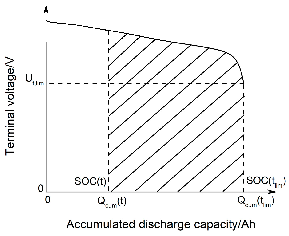
Therefore, the second category of the RDE prediction methods aims to obtain the specific value of RDE directly, and is more suitable for the remaining range prediction than SOE [10,11]. These methods determine the present and cutoff SOC value as the prediction domain at the beginning, and then directly estimate the RDE value by integrating the future terminal voltage, current, and time, assuming that the future working condition is known. In this way, there is no need to consider the dissipation of heat. As shown Figure 1, the RDE of the battery refers to the area of the shaded portion surrounded by the terminal voltage, U_t, and the accumulated discharge capacity, Q_cum. The current time, t, is the starting point of the remaining energy prediction. The corresponding SOC value is denoted as SOC(t), and the previously accumulated discharge capacity is Q_cum(t). The time, t_lim, is the cutoff moment of the discharge process, and the corresponding SOC and cumulative discharge capacity are SOC(t_lim) and Q_cum(t_lim), respectively. Therefore, the calculation of the remaining energy, E_RDE, of the battery is denoted as Equation (1):

$$E_{\mathrm{RDE}}=\underset{t}{\overset{t_{\lim }}{{\displaystyle \int }}}{U}_t\times I\times dt=\underset{{\mathrm{SOC}}_t}{\overset{{\mathrm{SOC}}_{\lim }}{{\displaystyle \int }}}{U}_t\times Q_a\times d\mathrm{SOC},$$

(1)

Based on the aforementioned definition and calculation method of RDE, Liu et al. [11] proposed a predictive-adaptive prediction method combining the real-time parameter identification and the future parameter prediction together. The dynamic terminal voltage in the future discharge process is predicted by a battery model based on the future load and the current battery state estimation result, then the E_RDE is estimated by accumulating the predicted voltage sequence. During the working condition, the battery model parameters are updated in real-time to optimize the voltage and E_RDE prediction results. However, this method only considered the RDE prediction for a battery cell and did not consider the battery pack situation where parameter and state inconsistency exists.

As can be seen from the above analysis, the key issue of RDE prediction is to establish a model which can predict the battery terminal voltage precisely, and estimate the model parameters and SOC accurately. Significant progress has been made in the study of single cell model parameter identification and the SOC estimation problem in recent years [12,13,14,15,16,17,18,19,20,21,22,23,24,25]. A commonly used method is to establish an ECM [13], which consists of a pure ohmic resistor and several resistor-capacitor (RC) parallel links, to describe the single cell. The parameters of the RC components are identified by experimental data through offline algorithms, such as least square algorithm [14,15,16], genetic algorithm [17,18,19,20], particle swarm optimization algorithm [21], and online identified by the recursive least square algorithm [22,23]. An adaptive filtering algorithm, such as the extended Kalman filter (EKF) [24,25], is then used to estimate the SOC based on the battery cell model and parameter identification results. This method has been widely verified to be effective and is also implemented in this research. However, for the battery state estimation, the inconsistency problem among battery cells is still a critical problem and needs to be studied.

Most of the existing research on battery pack state estimation considers the pack as a large cell and ignores the inconsistency between cells [26,27,28]. However, when estimating the RDE of a battery pack, the inconsistency between cells is not negligible. The inconsistency between cells includes various aspects, such as the SOC [29], internal resistance [30], model parameters, capacity [31], and temperature [32,33]. These inconsistencies can cause the entire battery pack’s discharge process to cease once a single cell reaches the discharge cutoff point. This short board effect reduces the available RDE of a battery pack. Therefore, in the issue of battery pack RED prediction, considerations of inconsistency must be added. In the literature considering such inconsistency, the straightforward method is to establish an independent battery model for each of the individual cells, and to independently estimate the state of each cell in the algorithm [34]. This method is complicated to operate and is not suitable for vehicle applications. To simplify the complexity of the model and algorithm, a “mean and difference” (M&D) model is proposed [35], which consists of a virtual “mean cell” model that describes the average state of the pack and “difference models” that represent the state difference between each cell and the mean cell. Based on the state estimation result of the mean cell, the state of each cell is acquired by adding the difference to the mean state. Dai [36] defined ΔSOC as the SOC difference between each cell and the mean SOC of the battery pack, and performed the SOC estimation through a dual time-scale extended Kalman filter algorithm. An accurate SOC estimation of each cell in the battery pack was achieved. However, although the SOC estimation of battery pack has been studied, in the RDE prediction problem, it is also necessary to consider the parameter inconsistency between cells, as the RDE is determined by the future terminal voltage.

In this paper, considering model complexity and accuracy, a “specific and difference” (S&D) model is proposed, and the advantage of this model compared with the M&D model is analyzed. To simultaneously and accurately estimate the SOC and parameters of each cell, a dual time-scale dual-EKF (DTSDEKF) algorithm is applied. The remainder of the paper is organized as follows: In Section 2, the characteristics of battery model parameter inconsistency are analyzed and the S&D model for a serial-connected battery pack is established based on the analysis. In Section 3, a DTSDEKF algorithm is introduced for the SOC and R₀ estimation of each cell in the battery pack, and the battery pack RDE prediction method is established based on the state estimation result. The implementation of the state estimation and RDE prediction algorithm is introduced in Section 4, and two dynamic working conditions, namely the NEDC and UDDS condition, are used to verify the effectiveness of the proposed method. The results are shown and the difference between the S&D and M&D model is discussed in Section 5. Section 6 gives the conclusions.

2. Battery Pack Modeling Approach Considering Inconsistency

2.1. Battery Cell Model Description

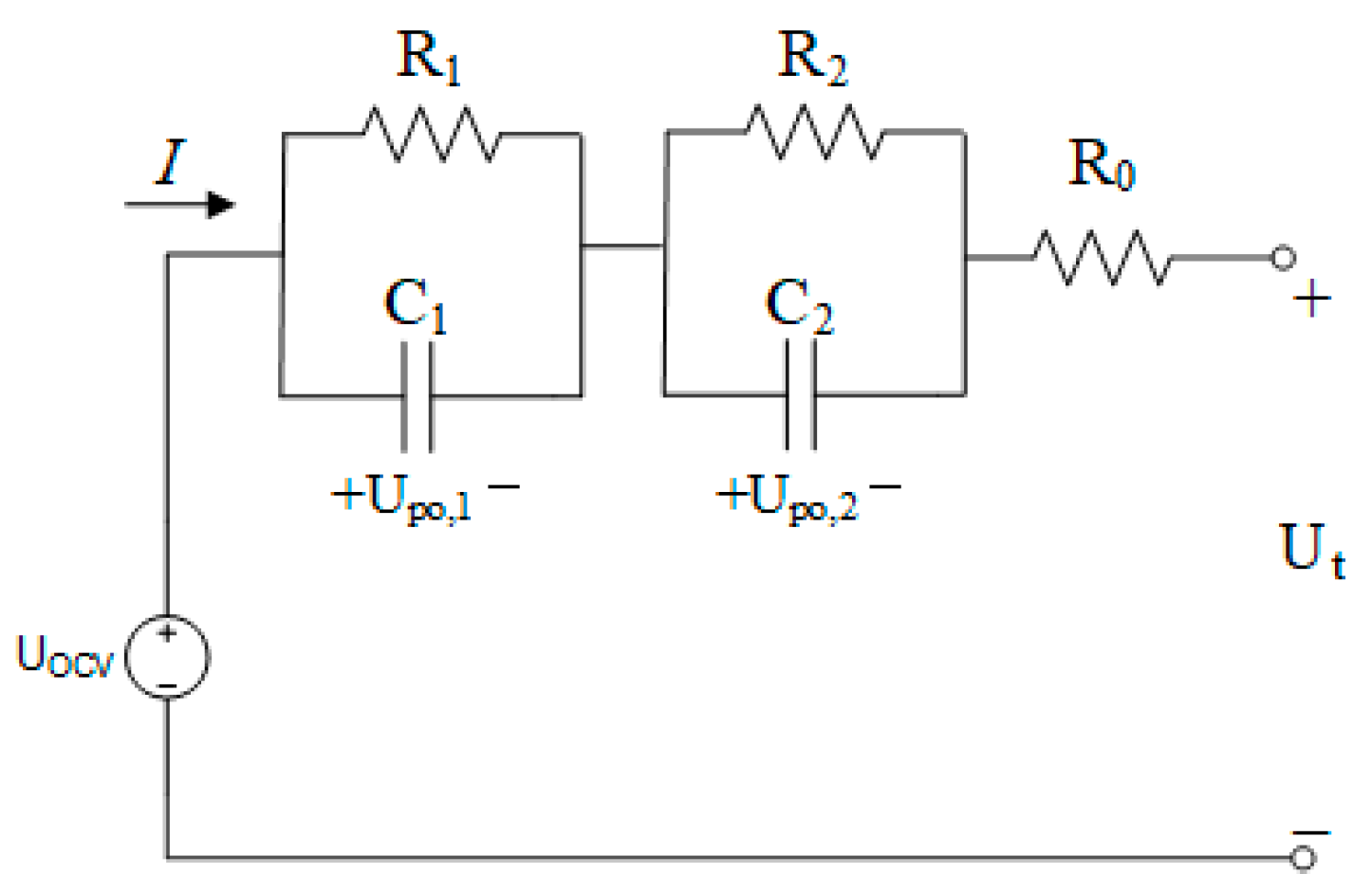
The accurate real-time SOC estimation, terminal voltage prediction, and RDE prediction are based on the precise battery model. As the driving range in real vehicle applications requires long-time estimation, considering the computational complexity and accuracy of the model, a second-order ECM with two RC components, which is commonly used in the laboratory, is selected in this paper. A second-order ECM consists of three parts, as shown in Figure 2:

• The source of voltage, U_OCV: Namely the open circuit voltage (OCV) of the battery. In this paper, an interpolation method, which is commonly used in real-time applications, is applied to calculate the OCV based on the estimated SOC by the look-up table denoting the relationship between SOC and OCV.
• The ohmic internal resistance, R₀: Consists of electrode material, electrolyte, internal resistance of the diaphragm, and contact resistance of each part.
• Two RC links: R₁ and R₂ are polarization resistance, indicating resistance caused by electrochemical polarization and concentration polarization. They connect with polarization capacitances, C₁ and C₂, in parallel and form RC links to simulate battery polarization and the diffusion effect.

In Figure 2, I is the current of the battery cell. It is defined that the discharging current is positive, while the charging current is negative. U_t is the terminal voltage of the battery cell at time, t, U_po,1 and U_po,2 are the polarization voltage corresponding to the RC link. The current and the terminal voltage are taken as the model input and output, respectively. The mathematical relationship between the cell current and terminal voltage is shown in Equation (2). The calculation of the polarization voltage is shown in Equation (3). τ_n is the time constant of each RC link and its calculation formula is shown in Equation (4). The SOC at time, t, is calculated as Equation (5) shows:

$$U_t=U_{OCV}\left({\mathrm{SOC}}_t\right)-I_t\times R_0-U_{t,po,1}-U_{t,po,2}$$

(2)

$$U_{t,po,n}=U_{t-1,po,n}\times e^{-\frac{\mathsf{\Delta }t}{{\tau }_{t-1,n}}}+I_t\times R_{t-1,n}\cdot \left(1-e^{-\frac{\mathsf{\Delta }t}{{\tau }_{t-1,n}}}\right)\hspace{1em}\hspace{1em}\left(n=1,2\right)$$

(3)

$${\tau }_n=R_n\times C_n\hspace{1em}\hspace{1em}\left(n=1,2\right)$$

(4)

$${\mathrm{SOC}}_t={\mathrm{SOC}}_{t-1}-\frac{I_t\times \mathsf{\Delta }t}{Q}$$

(5)

where SOC_t and SOC_t−1 denote the SOC at time, t, and time, (t−1); I_t represents the current at time, t; Δt is the sampling period; and Q denotes the capacity of the battery cell.

2.2. Off-Line Identification of Model Parameters Based on Genetic Algorithm

In the second-order EMC model, five parameters need to be identified, namely the R₀, R₁, R₂, C₁, and C₂. Due to the large number of identification parameters, it is necessary to apply an algorithm with good convergence and high robustness. Commonly used methods include the genetic algorithm (GA), particle swarm optimization (PSO), ant colony optimization (ACO), and so on. All of them belong to evolutionary algorithms that simulate natural behaviors. They all can start from a random solution and perform multiple iterations to find the optimal solution. However, it is easy for the PSO algorithm to fall into the local optimal solution and the algorithm is unstable. The ACO algorithm converges slowly. As a global optimization algorithm, the GA algorithm overcomes the shortcomings of easily falling into the local optimum and has a good global search ability. Therefore, the GA is applied in the model parameter identification.

In the parameter identification process, the root mean square error (RMSE) between the estimated terminal voltage and the actual terminal voltage is selected as the fitness function, f(x), as shown in Equation (6). To simplify the complexity of the parameter identification, it is considered that the voltage response from the stationary state to the first current pulse only reflects the response of the ohmic internal resistance, R₀. The constraint is added as Equation (7). Furthermore, the upper and lower limits, lb and ub, of x are adjusted by the empirical value, as shown in Equation (8). Through this method, the model parameters are identified at every 10% SOC point, and the relationship between the SOC and model parameters is obtained. In the state estimation algorithm, similar to the interpolation method of OCV, the value of the model parameters is also obtained by interpolating the estimated SOC value.

$$\min f\left(x\right)=\sqrt{\frac{{{\displaystyle \sum }}_{i=1}^n{\left( U_{t,e}^i-U_{t,a}^i\right)}^2}{n}}$$

(6)

$$s.t.\hspace{1em}\hspace{1em}\hspace{1em}I\left(2\right)\cdot x\left(1\right)=U\left(1\right)-U\left(2\right)$$

(7)

$$\mathrm{lb}\le x\le \mathrm{ub}$$

(8)

2.3. S&D Model of Battery Pack

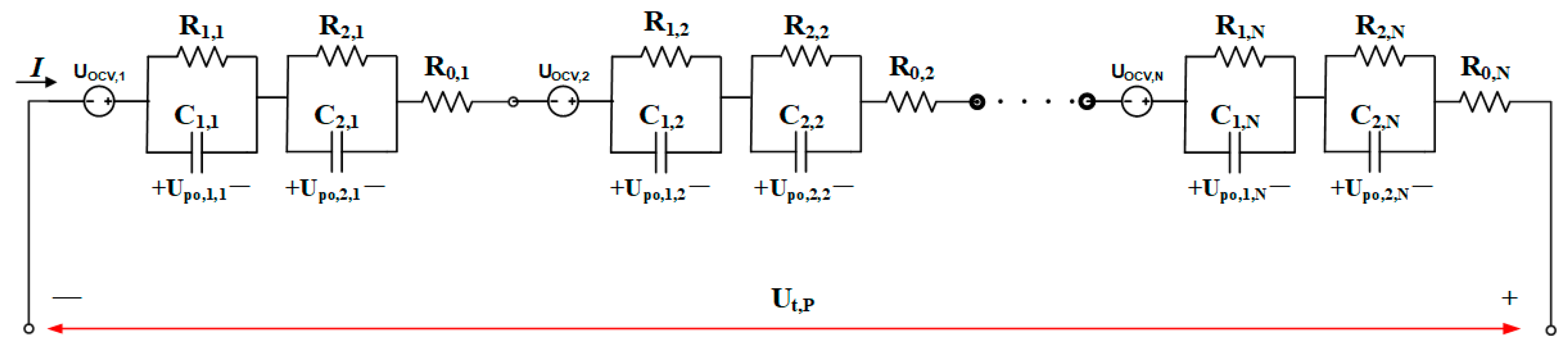
As shown in Figure 3, a typical battery pack consisting of N cells can be represented by N second-order ECMs connected in series. The process of the S&D model constitution is divided into four stops.

1. Specific Cell Model Establishment

Firstly, one cell within the battery pack is selected as the specific cell and the specific model is denoted by Equations (2)–(5). Theoretically, any cell within the pack can be chosen as the specific cell. For example, if the cell with the highest voltage or the cell with the lowest SOC is selected, in both cases, the results of each cell’s state estimation will not be different, as long as the estimation results are accurate. In this research, considering that the discharge cutoff point is determined by the cell with the lowest voltage, and that the voltage can be conveniently and accurately obtained in practical applications, the cell with the lowest voltage at the beginning of the estimation process is selected as the specific one. Therefore, the specific cell model could be described by adding the subscript, s, in Equations (2)–(5), which indicates the state of the specific cell.

2. Inconsistency Analysis

Secondly, different kinds of inconsistences are analyzed. The inconsistency between cells includes various aspects, such as SOC, model parameters, capacity, and temperature. However, the degree of inconsistency (DOI) of different factors and the impact on battery RDE estimation are different. In practical applications, if all the inconsistencies are considered and the corresponding difference model is established, the algorithm will be too complicated and impractical.

In this study, 40 INR18650-29E lithium-ion batteries produced by Samsung SDI are used as the research object. The basic parameters are shown in

Table 1. Specifications of the battery used in this research.

Subject	Specification
Nominal Voltage/V	3.62
Nominal Capacity/Ah	2.9
Electrode chemistry	NCA/graphite
Internal resistance/mΩ	45
Dimension/mm	Diameter: 18.40 Height: 65.02
Storage temperature/℃	−20 to 25
Weight/g	45 g
Manufacturer	Samsung SDI

. Since all of them are new batteries produced in the same batch, the inconsistency of different cell’s SOC-OCV curve relationship is ignored. Meanwhile, this study does not consider the thermal model of batteries, so the temperature inconsistency is not considered, and relevant research will be carried out in the future.

Practically, the SOC inconsistency is the most common and direct factor affecting the state estimation of battery packs, so it will be the main consideration in this research.

The model parameter inconsistency includes two types. The first is the parameter inconsistency caused by the inconsistent SOC. This can be described by the difference model of SOC. The second type is the inconsistency of the relationships between the SOC and parameters, which would cause the model parameters, such as R₀, of different cells to be different from each other under the same SOC. This requires the algorithm to estimate the exact results of the parameters in real time and adaptively correct the relationship between the model parameters and the SOC. In this research, five model parameters, including R₀, R₁, R₂, C₁, and C₂, are established. Theoretically, all five parameters and the battery capacity should be inconsistent, but their DOIs are not the same. Therefore, to make the difference model more realistic, and to simplify the computational complexity as much as possible, the difference between the DOIs of the capacity and parameters is analyzed. The factor with the largest DOI is presented in the difference model, and the other factors are ignored.

To make them comparable, the coefficient of variation (CV) is used to characterize the DOI. The CV is a standardized measure for the dispersion of a probability distribution, which is defined as the ratio of the value of standard deviation, σ, to the mean, µ, (or its absolute value, |µ|), as shown in Equation (9). The advantage of the CV is that the effects of the dimension and average can be eliminated, so that different parameters’ DOIs can be compared directly.

$$\mathrm{CV}=\frac{\sigma }{\mu }$$

(9)

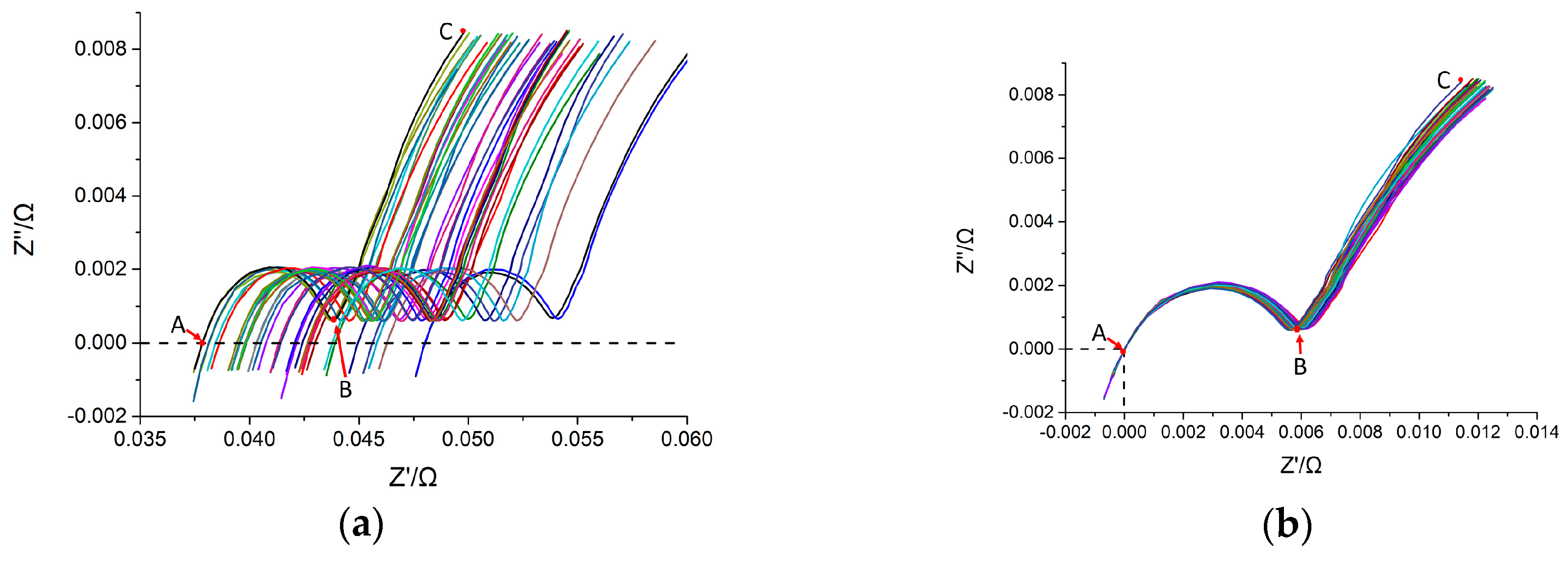
The general method for obtaining battery model parameters off-line is introduced in Section 2.2. However, this method is complicated and only suitable for accurate calibration of individual cells. To quickly analyze the model parameters of 40 cells, electrochemical impedance spectroscopy (EIS) is used in this research. EIS analysis produces disturbances through small amplitude alternating current (AC) signals, and observes the response of the battery to small signal disturbances at steady state, thereby obtaining the relationship between battery impedance and frequency [37]. In the Nyquist diagram of the impedance, the intersection of the curve and the real axis corresponds to the ohmic internal resistance, R₀, of the battery, including the internal resistance of the electrolyte, the diaphragm, the current collector, etc. In the second-order ECM, it is considered that the semicircle of the medium frequency band describes the charge transfer process, corresponding to the transfer resistance, R_ct, and the double layer capacitance, C_dl, that is, R₁ and C₁ of the RC link with the smaller time constant. The oblique line of the low frequency band corresponds to the R_diff and C_diff of the solid state diffusion process, that is, R₂ and C₂ of the RC link with the larger time constant [38].

We conducted EIS experiments on 40 cells at 25 °C and 50% SOC. The EIS curves are shown in Figure 4. To compare the inconsistency of the impedance between the cells in different frequency segments, the feature points are used to quantify them. The intersection of the EIS curve and the horizontal axis (point A), the inflection point of the semicircle (point B), and the right end point of the oblique line (point C) are selected to characterize the impedance at high frequency, medium frequency, and low frequency band, respectively. It can be seen from Figure 4a that the core difference among the 40 EIS curves is reflected in point A. Then, the curves are shifted to the left till point A of each line is at the origin of the coordinate axis, so that the inconsistency of point A is eliminated. As shown in Figure 4b, the semicircle can basically coincide after translation, and the oblique lines of the low frequency band show a slight inconsistency. That is to say, R₀ under high frequency is the core source of the impedance inconsistency, and the inconsistencies of the non-ohmic impedance portion represented by the semicircle and the oblique line in the medium and low frequency bands are not remarkable.

Each cell’s impedance mode, |Z|, corresponding to point A is calculated to represent R₀. Similarly, the mode from point A to point B and the mode from point A to point C are calculated to represent R₁, C₁ and R₂, C₂, respectively. The CV values of the three modes are calculated to compare different parameters’ DOIs. Meanwhile, the CV of 40 cells’ capacity values, which are calibrated at 25 °C under 1C discharge profile, is also calculated as the DOI of capacity. “C” is used to denote the current rate, and 1C is equal to the current rate by which the nominal capacity can be discharged from full to empty in 1 h; in other words, it is equal to 2.9 A in this paper. The results are shown in

Table 2. Coefficient of variation results of four variables.

Variable	CV
Mode of Point A (High frequency)	0.065
Mode from Point B to A (Intermediate frequency)	0.028
Mode from Point C to A (low frequency)	0.012
Capacity (@25 °C, 1C Discharge)	0.0033

.

It can be seen from the results that the CV of R₀ is more than twice the CV of the other three variables. Therefore, the inconsistency of R₀ is considered and each cell’s R₀ will be estimated in the algorithm, while the inconsistencies of the other parameters and capacity are ignored.

It should be noted that in the experiments, the test bench is controlled carefully to ensure that the contact resistance of each cell remains the same. Besides, the battery used in this research is 18650 format cells with a nominal capacity of 2.9Ah, which is relatively small compared to the large format batteries used in the EV battery packs. Therefore, the impedance of the battery cell is much larger. For the vehicle applications, the same process of the inconsistency analysis introduced in this research could be carried out to find out the actual main factor of the inconsistency and revise the algorithm accordingly.

3. Difference Model Establishment

From the above analysis, it is concluded that the SOC and R₀ inconsistencies should be considered in the battery pack model and the state estimation algorithm. The difference model of the other cells is shown in Equation (10):

$${\mathrm{SOC}}_i={\mathrm{SOC}}_s+\mathsf{\Delta }{\mathrm{SOC}}_i\hspace{1em}\hspace{1em}\hspace{1em}(i=1,2,\cdots ,N-1)$$

(10)

where SOC_min and SOC_i denote the specific cell and the i-th cell’s SOC value, respectively. The ΔSOC_i represents the SOC difference between the i-th cell and the specific cell. In this way, the i-th cell could be described using Equations (11)–(14):

$$U_{t,i}=U_{OCV}\left({\mathrm{SOC}}_{t,i}\right)-I_t\cdot R_{0,i}-U_{t,po,1,i}-U_{t,po,2,i}$$

(11)

$$U_{t,po,n,i}=U_{t-1,po,n,i}\cdot e^{-\frac{\mathsf{\Delta }t}{{\tau }_{t-1,n,i}\left(SO{C}_{t-1,i}\right)}}+I_t\cdot R_{t-1,n,i}\left({\mathrm{SOC}}_{t-1,i}\right)\cdot \left(1-e^{-\frac{\mathsf{\Delta }t}{{\tau }_{t-1,n,i}\left({\mathrm{SOC}}_{t-1,i}\right)}}\right)\hspace{1em}\hspace{1em}\left(n=1,2\right)$$

(12)

$${\tau }_{n,i}\left({\mathrm{SOC}}_i\right)=R_{n,i}\left({\mathrm{SOC}}_i\right)\cdot C_{n,i}\left({\mathrm{SOC}}_i\right)\hspace{1em}\hspace{1em}\left(n=1,2\right)$$

(13)

$${\mathrm{SOC}}_{t,i}={\mathrm{SOC}}_{t-1,i}-\frac{I_t\cdot \mathsf{\Delta }t}{Q_s}$$

(14)

where the subscript, i, in the equations indicates the state of the other cell, and i equals from 1 to N−1, as the specific cell is excluded. The meaning of the variables are the same as in Equations (2)–(5). Q_s is the capacity of the specific cell because the capacity inconsistency is ignored as analyzed and the capacity of all cells is regarded as the same.

It should be noted that the R₁, R₂, C₁, and C₂ of the i-th cell are still inconsistent with other cells at the same time, because of their different SOC. Therefore, these inconsistencies are manifested by ΔSOC, and in the state estimation algorithm, they can be directly estimated by interpolating the SOC-parameter look-up table of the specific cell. The value of each cell’s R₀ should be estimated online in the algorithm, as analyzed in the last step.

4. Battery Pack Description by the S&D Model

In terms of battery pack modeling, the terminal voltage of an N cells series-connected battery pack, which is denoted as U_p, can be calculated with the sum of the cell terminal voltage calculated for specific cell and other cells, as shown in Equation (15):

$$U_{t,P}={\displaystyle \sum _{i=1}^N\left(U_{\mathrm{OCV}}\left({\mathrm{SOC}}_{t,i}\right)-I_t\cdot R_{0,i}-U_{t,po,1,i}-U_{t,po,2,i}\right)}$$

(15)

3. RDE Estimation Method for Battery Pack Considering SOC and R₀ Inconsistency

As analyzed in the introduction section, an accurate estimation of the SOC and model parameters of each individual cell in the battery pack is the first step for predicting the RDE of a battery pack. Then, the future SOC, model parameters, and terminal voltage of each cell can be predicted based on a given future operating condition and the calibrated SOC-parameter look-up table. Finally, the RDE of the battery pack is predicted by accumulating the future terminal voltage of the battery pack.

3.1. Dual Time-Scale Battery Pack SOC and R₀ Estimation Method

3.1.1. First Time Scale—Specific Cell

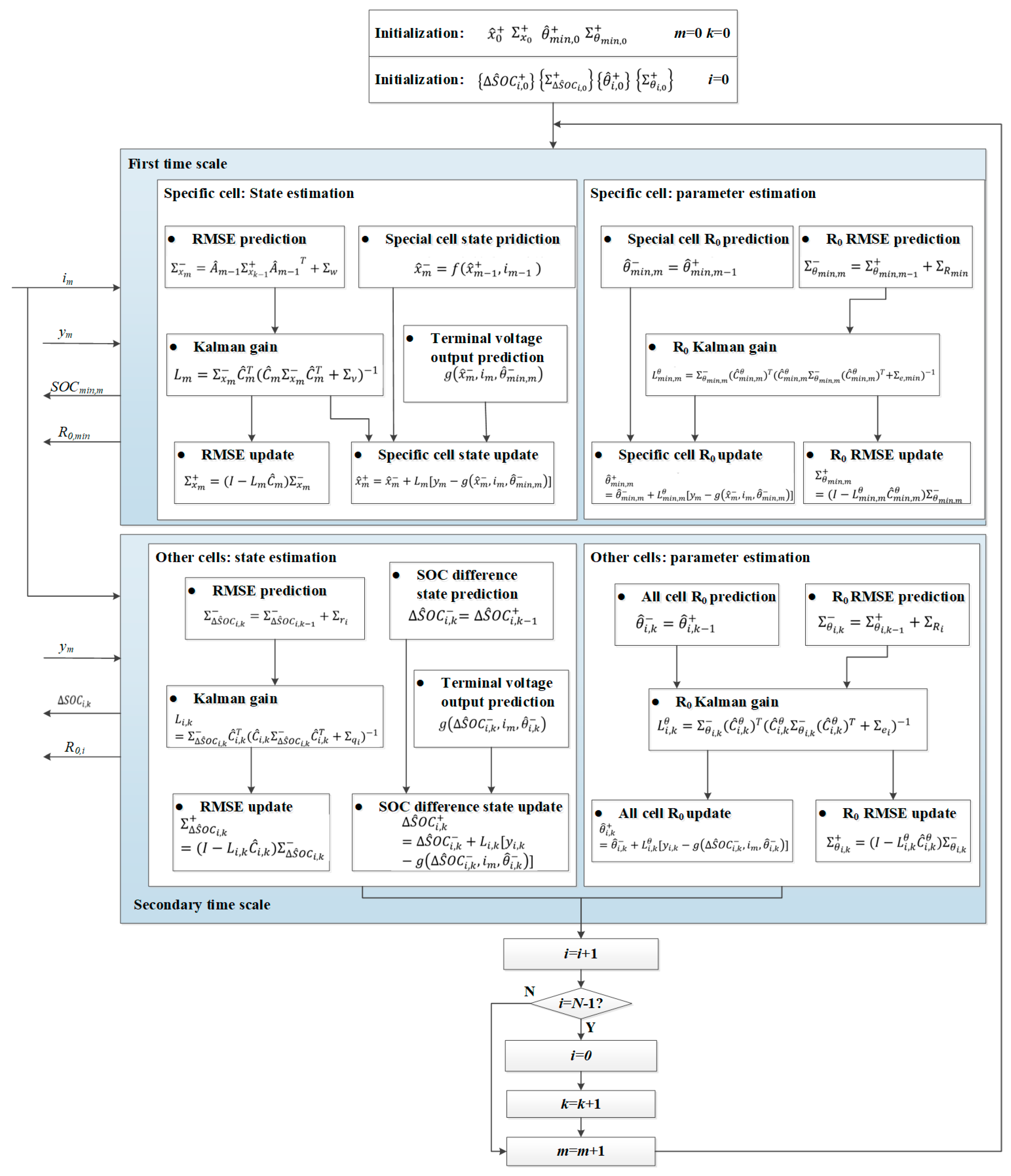
The Kalman filter is one of the commonly used techniques for SOC estimation [24,25,26,27,28]. Considering the nonlinear characteristics of the battery model, the EKF algorithm is utilized in this research. This filter assumes a priori knowledge of the process and the measurement noise covariance. In order to estimate the SOC and model parameter, R₀, of the specific cell simultaneously, a dual extended Kalman filter (DEKF) algorithm is used in the first time scale. The first EKF is used to estimate the SOC and the second is used to estimate the R₀ of the specific cell. In the DEKF algorithm, the state equation and output observation equation of the system is established as Equations (16)–(19) shows:

$$x_{k+1}=f\left(x_k,u_k,{\theta }_k\right)+w_k$$

(16)

$$y_k=g\left(x_k,u_k,{\theta }_k\right)+{\nu }_k$$

(17)

$${\theta }_{k+1}={\theta }_k+r_k$$

(18)

$$y_k=g\left(x_k,u_k,{\theta }_k\right)+e_k$$

(19)

where x_k is the state variable of the system, u_k is the input of the system, θ_k is the time-varying parameter vector, and y_k is the output of the system. w_k, ν_k, and e_k are the state noise and measurement noise of the system, and they are independent. r_k is a small perturbation, indicating the slow time-varying characteristics of the parameters. f(x_k, u_k, θ_k) and g(x_k, u_k, θ_k) are the nonlinear state equation and output equation of the system.

For nonlinear systems, suppose f(x_k, u_k, θ_k) and g(x_k, u_k, θ_k) are divisible at all operating points and can be linearized by first-order Taylor approximation to obtain parameter matrices, including A_k and C_k. The linearization processes are shown in Equations (20)–(25):

$$f\left(x_k,u_k,{\theta }_k\right)\approx f\left(x_k,u_k,{\widehat{\theta }}_k\right)+{\frac{\partial f\left(x_k,u_k,{\widehat{\theta }}_k\right)}{\partial x_k}|}_{x_k={\widehat{x}}_k}\left(x_k-{\widehat{x}}_k\right)$$

(20)

$$g\left(x_k,u_k,{\theta }_k\right)\approx g\left(x_k,u_k,{\widehat{\theta }}_k\right)+{\frac{\partial g\left(x_k,u_k,{\widehat{\theta }}_k\right)}{\partial x_k}|}_{x_k={\widehat{x}}_k}\left(x_k-{\widehat{x}}_k\right)$$

(21)

$$\left(x_k,u_k,{\theta }_k\right)\approx g\left({\widehat{x}}_k,u_k,{\theta }_k\right)+{\frac{\partial g\left({\widehat{x}}_k,u_k,{\theta }_k\right)}{\partial {\theta }_k}|}_{{\theta }_k={\widehat{\theta }}_k}\left({\theta }_k-{\widehat{\theta }}_k\right)$$

(22)

$${\widehat{A}}_{k-1}={\frac{\partial f\left(x_{k-1},u_{k-1},{\widehat{\theta }}_k^{-}\right)}{\partial x_{k-1}}|}_{x_{k-1}={\widehat{x}}_{k-1}^{+}}$$

(23)

$${\widehat{C}}_k={\frac{\partial g\left(x_k,u_k,{\widehat{\theta }}_k^{-}\right)}{\partial x_{k-1}}|}_{x_{k-1}={\widehat{x}}_{k-1}^{+}}$$

(24)

$${\widehat{C}}_k^{\theta }={\frac{\partial g\left({\widehat{x}}_k,u_k,\theta \right)}{\partial \theta }|}_{{\theta }_k={\widehat{\theta }}_k^{-}}$$

(25)

After linearization, the SOC and R₀ of the specific cell is estimated according to the DEKF algorithm shown in

Table 3. Process of DEKF algorithm.

Step 1: Initialization

${\widehat{x}}_0^{+}=E\left(x_0\right),{\mathsf{\Sigma }}_{x_0}^{+}=E\left[\left(x_0-{\widehat{x}}_0^{+}\right){\left(x_0-{\widehat{x}}_0^{+}\right)}^T\right],{\widehat{\theta }}_0^{+}=E\left({\theta }_0\right),{\mathsf{\Sigma }}_{{\theta }_0}^{+}=E\left[\left({\theta }_0-{\widehat{\theta }}_0^{+}\right){\left({\theta }_0-{\widehat{\theta }}_0^{+}\right)}^T\right]$ ${\mathsf{\Sigma }}_w=E\left(w\times w^T\right),{\mathsf{\Sigma }}_{\nu }=E\left(\nu \times {\nu }^T\right),{\mathsf{\Sigma }}_R=E\left(R\times R^T\right),{\mathsf{\Sigma }}_e=E\left(e\times e^T\right)$

Step 2: Iteration and calculation of the two EKF:

State and parameter update according to the last iteration result: ${\widehat{\theta }}_k^{-}={\widehat{\theta }}_{k-1}^{+},{\mathsf{\Sigma }}_{{\theta }_k}^{-}={\mathsf{\Sigma }}_{{\theta }_{k-1}}^{+}+{\mathsf{\Sigma }}_R$ ${\widehat{x}}_k^{-}=f\left({\widehat{x}}_{k-1}^{+},u_{k-1},{\widehat{\theta }}_k^{-}\right),{\mathsf{\Sigma }}_{x_k}^{-}={\widehat{A}}_{k-1}{\mathsf{\Sigma }}_{x_{k-1}}^{+}{\widehat{A}}_{k-1}{}^T+{\mathsf{\Sigma }}_w$

Kalman gain calculation and state estimation of the first EKF: $L_k={\mathsf{\Sigma }}_{x_k}^{-}{\widehat{C}}_k^T{\left({\widehat{C}}_k{\mathsf{\Sigma }}_{x_k}^{-}{\widehat{C}}_k^T+{\mathsf{\Sigma }}_{\nu }\right)}^{-1}$ ${\widehat{x}}_k^{+}={\widehat{x}}_k^{-}+L_k\left[ y_k-g\left({\widehat{x}}_k^{-},u_k,{\widehat{\theta }}_k^{-}\right)\right]$ ${\mathsf{\Sigma }}_{x_k}^{+}=\left(I-L_k{\widehat{C}}_k\right){\mathsf{\Sigma }}_{x_k}^{-}$

Kalman gain calculation and parameter estimation of the second EKF: $L_k^{\theta }={\mathsf{\Sigma }}_{{\theta }_k}^{-}{({\widehat{C}}_k^{\theta })}^T{\left({\widehat{C}}_k^{\theta }{\mathsf{\Sigma }}_{{\theta }_k}^{-}{({\widehat{C}}_k^{\theta })}^T+{\mathsf{\Sigma }}_e\right)}^{-1}$ ${\widehat{\theta }}_k^{+}={\widehat{\theta }}_k^{-}+L_k^{\theta }\left[y_k-g\left({\widehat{x}}_k^{-},u_k,{\widehat{\theta }}_k^{-}\right)\right]$ ${\mathsf{\Sigma }}_{{\theta }_k}^{+}=\left(I-L_k^{\theta }{\widehat{C}}_k^{\theta }\right){\mathsf{\Sigma }}_{{\theta }_k}^{-}$

. The state space expression of the specific cell is shown in the following equations:

$$\left(\begin{array}{c}{\mathrm{SOC}}_{k,s}\\ U_{po,1,k,s}\\ U_{po,2,k,s}\end{array}\right)=\left(\begin{array}{ccc}1& & \\ & e^{-\mathsf{\Delta }t/{\tau }_1}& \\ & & e^{-\mathsf{\Delta }t/{\tau }_2}\end{array}\right)\times \left(\begin{array}{c}{\mathrm{SOC}}_{k-1,s}\\ U_{po,1,k-1,s}\\ U_{po,2,k-1,s}\end{array}\right)+\left(\begin{array}{c}-\mathsf{\Delta }t/Q_s\\ R_{1,s}\left(1-e^{-\mathsf{\Delta }t/{\tau }_1,s}\right)\\ R_{2,s}\left(1-e^{-\mathsf{\Delta }t/{\tau }_{2,s}}\right)\end{array}\right)i_k$$

(26)

$$U_{k,s}=U_{OCV}\left({\mathrm{SOC}}_{k,s}\right)-i_k{R}_{0,s}-U_{po,1,k,s}-U_{po,2,k,s}$$

(27)

$${\widehat{A}}_{k,s}=diag\left(1,\exp \left(-\mathsf{\Delta }t/{\tau }_{1,s}\right),\exp \left(-\mathsf{\Delta }t/{\tau }_{2,s}\right)\right)$$

(28)

$${\widehat{B}}_{k,s}={\left(\begin{array}{ccc}-\mathsf{\Delta }t/Q_s& R_{1,s}\left(1-e^{-\mathsf{\Delta }t/{\tau }_{1,s}}\right)& R_{2,s}\left(1-e^{-\mathsf{\Delta }t/{\tau }_{2,s}}\right)\end{array}\right)}^T$$

(29)

$${\widehat{C}}_{k,s}=\left(\begin{array}{ccc}{d\mathrm{OCV}/d\mathrm{SOC}|}_{{\widehat{\mathrm{S}}\mathrm{OC}}_{k,s}}& -1& -1\end{array}\right)$$

(30)

$$\begin{array}{ll}{\widehat{C}}_{k,s}^{\theta }& ={\frac{dg\left({\widehat{x}}_{k,s},u_{k,s},\theta \right)}{\partial \theta }|}_{{\theta }_k={\widehat{\theta }}_k^{-}}=\frac{\partial g\left({\widehat{x}}_{k,s},u_{k,s},\theta \right)}{\partial \theta }+\frac{\partial g\left({\widehat{x}}_{k,s},u_{k,s},\theta \right)}{\partial {\widehat{x}}_{k,s}^{-}}\frac{d{\widehat{x}}_{k,s}^{-}}{d\theta }\\ & =\frac{\partial g\left({\widehat{x}}_{k,s},u_k,\theta \right)}{\partial R_{k,s}}+\frac{\partial g\left({\widehat{x}}_{k,s},u_{k,s},\theta \right)}{\partial {\widehat{x}}_{k,s}^{-}}\times \frac{d{\widehat{x}}_{k,s}^{-}}{dR}=\frac{\partial g\left({\widehat{x}}_{k,s},u_{k,s},\theta \right)}{\partial R_{k,s}}=-i_k\end{array}$$

(31)

3.1.2. Second Time Scale—Other Cells

The difference model for the i-th cell is defined in Section 2. To estimate the ΔSOC and R₀ of the i-th cell, a DEKF algorithm is also implemented, and the calculation process is similar to that in Table 3. Although the computational complexity of the single-state Kalman filter is low, simultaneously updating the ∆SOC_i and R_0,i of each individual in the pack means that the computational complexity is multiplied. Considering that the SOC difference between cells and the R₀ of each cell both change slowly, an algorithm that updates only one cell at a time is applied. Assuming that there are N cells in the pack, there are N−1 cells’ ∆SOC_i and R_0,i need to be estimated in the second time scale. The state estimation function can be written as:

$$\mathsf{\Delta }{\mathrm{SOC}}_{k+1,i}=\mathsf{\Delta }{\mathrm{SOC}}_{k,i}+r_{k,i}$$

(32)

$$U_{k,i}=\mathrm{OCV}\left({\mathrm{SOC}}_{m,s}+\mathsf{\Delta }{\mathrm{SOC}}_{k,i}\right)-i_m{R}_{0,i}^k-U_{po1,s}^m-U_{po2,s}^m+q_{k,i}$$

(33)

$$m=\left(N-1\right)\cdot k+i$$

(34)

where r_k,i represents the state noise, and refers to the possible fluctuations in the process of ∆SOC_i change, and q_k,i represents the external noise, and refers to the measurement error of the i-th cell. U_k,i represents the terminal voltage of the i-th cell.

The parameter matrix of the DEKF in the second time scale is shown in Equations (35) and (36):

$$\begin{array}{ll}{\widehat{C}}_{k,i}& ={\frac{d\mathrm{OCV}}{d\mathsf{\Delta }{\mathrm{SOC}}_i}|}_{\mathsf{\Delta }{\mathrm{SOC}}_i=\mathsf{\Delta }{\widehat{\mathrm{S}}\mathrm{OC}}_{i,k}^{-}}={\frac{d\mathrm{OCV}}{d({\mathrm{SOC}}_i-{\mathrm{SOC}}_s)}|}_{{\mathrm{SOC}}_i={\mathrm{SOC}}_s+\mathsf{\Delta }{\widehat{\mathrm{S}}\mathrm{OC}}_{k,i}^{-}}\\ & ={\frac{d\mathrm{OCV}}{d{\mathrm{SOC}}_i}\cdot \frac{d{\mathrm{SOC}}_i}{d({\mathrm{SOC}}_i-{\mathrm{SOC}}_s)}|}_{{\mathrm{SOC}}_i={\mathrm{SOC}}_s+\mathsf{\Delta }{\widehat{\mathrm{S}}\mathrm{OC}}_{k,i}^{-}}={\frac{d\mathrm{OCV}}{d{\mathrm{SOC}}_i}|}_{{\mathrm{SOC}}_i={\mathrm{SOC}}_s+\mathsf{\Delta }{\widehat{\mathrm{S}}\mathrm{OC}}_{k,i}^{-}}\end{array}$$

(35)

$${\widehat{C}}_{k,i}^{\theta }=-i_m$$

(36)

where ${\widehat{C}}_{k,i}$ represents the derivative of the open circuit voltage versus ∆SOC_i. By deriving Equation (35), that is, dOCV/d∆SOC_i is equivalent to dOCV/dSOC_i, which is the first derivative of OCV with respect to SOC. Considering that the SOC-OCV curve used in this research is not a continuous curve, but a discrete look-up table obtained by experimental calibration, the dOCV/d∆SOC_i value is calculated using the same method of calculating dOCV/dSOC_s used in the specific cell.

Figure 5 is the flow chart of the dual time-scale dual EKF (DTSDEKF) algorithm proposed for a battery pack. In each cycle, the first time scale is used for the iterative update of the SOC state and R₀ of the specific cell, which has the lowest voltage at the beginning of the estimation process, while the second time scale is used for the iterative update of the ∆SOC_i and R_0,i of the other cells. The update period of each cell is N−1 times.

3.2. Predictive-Adaptive Method for Battery Pack Terminal Voltage Prediction

As shown in [11], a predictive-adaptive method combining the real-time parameter identification and the future parameter prediction is suitable for the RDE prediction of lithium-ion batteries. In this research, a similar method is implemented based on the offline parameter identification results and online SOC and R₀ estimation algorithm for battery packs.

According to the analysis in Section 2, the relationship between the SOC and model parameters, including R₁, R₂, C₁, and C₂, of different cells is considered consistent and remains unchanged during the estimation process. Therefore, it is only necessary to adaptively predict R₀ in the algorithm and the other parameters can be predicted based on the offline calibrated SOC-parameter table and the predicted future SOC value under the given working condition.

As the DTSDEKF algorithm is used here to simultaneously estimate the SOC and R₀ of each cell in real-time, the adaptive correction and prediction process of R₀ could be denoted as Equations (37) and (38):

$$\mathsf{\Delta }{R}_0=R_{0,a}\left(\mathrm{SOC}\left(t_{present}\right)\right)-R_{0,Cali}\left(\mathrm{SOC}\left(t_{present}\right)\right)$$

(37)

$$R_0\left(\mathrm{SOC}\left(t_{pre}\right)\right)=R_{0,Cali}\left(\mathrm{SOC}\left(t_{pre}\right)\right)+\mathsf{\Delta }{R}_0$$

(38)

where R_0,a(SOC(t_present)) refers to the estimated R₀ under the present SOC by the algorithm. R_0,cali(SOC(t_present)) refers to the corresponding R₀ calculated by interpolating the SOC-R₀ table under the present SOC. ∆R₀ is the difference between the two values. The SOC-R₀ curve is then translated by ∆R₀ as a new reference for future parameters in the future prediction, and the predicted R₀ is denoted by R₀(SOC(t_pre)).

The future SOC value under the given working condition is predicted by using the ampere-hour integration method in Equation (39):

$$\mathrm{SOC}\left(t_{pre}\right)=\mathrm{SOC}\left(t_{present}\right)-\frac{{{\displaystyle \int }}_t^{t_{pre}}\eta I_{pre}dt}{Q_a}$$

(39)

where SOC(t_present) is the estimated present SOC value. η is the coulomb efficiency, which is set as 1 in this research. Q_a is the actual capacity of the battery and is equal to Q_s here.

The current polarization voltage value estimated by the DEKF algorithm is used as the starting value of the prediction process, and the calculation formula of the polarization voltage is as shown in Equation (40). The terminal voltage is calculated as Equation (41):

$$U_{po,i}\left(t_{pre}\right)=I\left(t_{pre}\right)R_i\left(t_{pre}\right)\left[1-exp\left(-\frac{t_{pre}}{{\tau }_i\left(t_{pre}\right)}\right)\right],i=1,2$$

(40)

$$U_t\left(t_{pre}\right)=\mathrm{OCV}\left(\mathrm{SOC}\left(t_{pre}\right)\right)-I_{pre}\left(t_{pre}\right)\cdot R_o\left(t_{pre}\right)- U_{po,1}\left(t_{pre}\right)-U_{po,2}\left(t_{pre}\right)$$

(41)

The future terminal voltage of the battery pack is predicted by Equation (42):

$$U_{t,P}={\displaystyle \sum _{i=1}^N{U}_{t,i}}$$

(42)

3.3. RDE Prediction Method for Battery Pack

The RDE of the battery pack is predicted by accumulating the future terminal voltage of the battery pack. The key issue is to predict the future discharge cutoff point.

In the RDE prediction algorithm for a battery cell, the discharge cutoff point is predicted by utilizing the cell’s predicted future terminal voltage value, and when the cutoff condition is reached, such as 2.55 V, the moment is used as the cutoff point. However, in the algorithm for a battery pack, there will be significant error from using the battery pack voltage to predict the cutoff voltage of the discharging process, as the cells inside a battery pack do not reach the discharge cutoff point at the same time due to the inconsistency. When the terminal voltage of the battery pack approaches the cutoff point, the cell with the lowest voltage would have already been over-discharged. Therefore, unlike the definition of a cell’s cutoff point, the discharge cutoff point of a battery pack is determined by the first cell that reaches the cutoff point, thereby ensuring the performance, life, and reliability of the battery pack.

Finally, the RDE of the battery pack is equal to the integral of the current, time, and the terminal voltage of each cell from the starting point time till the discharge cutoff point of the battery, as shown in Equation (43):

$$E_{RDE,P}={\displaystyle \sum }_{i=1}^N\underset{t_0}{\overset{t_{lim}}{{\displaystyle \int }}}{U}_{t,i}\cdot I_{pre}\cdot \mathsf{\Delta }t$$

(43)

4. Experiments

To verify the proposed RDE prediction method for battery pack, 40 INR18650-29E lithium-ion batteries produced by Samsung SDI were used. The basic parameters are shown in Table 1. The experiments are divided into two categories. The first is the cell calibration test, including the calibration tests of the SOC-OCV curve and the model parameters. The second is the battery pack test. In this experiment, two dynamic working conditions, including the NEDC and Urban Dynamometer Driving Schedule (UDDS), were used to verify the effectiveness of the battery RDE estimation algorithm when there is inconsistency in the battery pack.

4.1. Battery Cell Tests

The calibration tests for SOC-OCV curve and model parameters were carried out using the Chroma 17011 Regenerative Battery Test System. The environmental temperature was controlled at 25 °C by a Votsch C4-180 environmental chamber.

The SOC-OCV test was carried out by charging and discharging a cell using constant current (CC) of 1/25 C. The cell was regarded as fully charged when charged to 4.2 V and fully discharged when discharged to 2.55 V. The average value of the obtained continuous charge and discharge voltage curve data is taken as the equilibrium OCV curve data. Additionally, the set of the curve data was segmented to obtain 201 calibration points, forming an approximately continuous SOC-OCV curve.

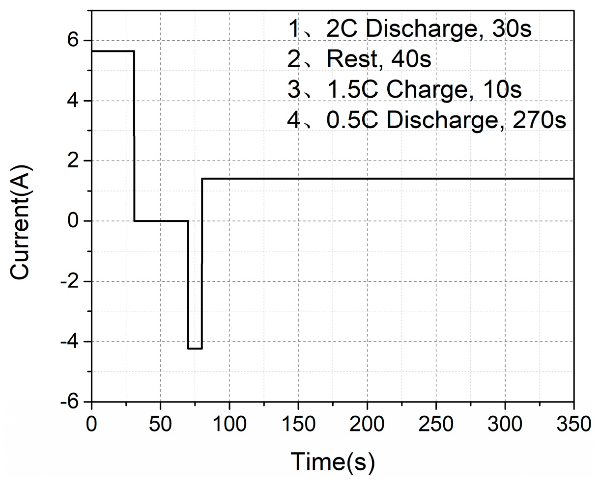
Starting from SOC = 100%, the Hybrid Pulse Power Characterization (HPPC) test condition, which is shown in Figure 6, was performed every 10% SOC, and the obtained current input and terminal voltage output data were subjected to parameter identification in the second-order ECM by the genetic algorithm, as introduced in Section 2.2.

4.2. Battery Pack Tests

The working condition tests for the battery pack were carried out using the Chroma 17020 Regenerative Battery Test System. All tests were carried out under 25 °C.

Eight cells with the same capacity of 2.8 Ah were selected and serially connected, and the initial SOC inconsistency was artificially constructed. To make the influence of the SOC inconsistency more obvious and to verify the effectiveness of the algorithm, the interval of the SOC between each cell was set to approximately 5%. The approximate initial SOC value distribution is shown in the following table (

Table 4. Designed SOC distribution of the battery pack.

Cell Number	Approximate Initial SOC Value
1	65%
2	70%
3	75%
4	80%
5	85%
6	90%
7	95%
8	100%

). It should be noted that the actual value of each cell’s initial SOC was calculated at the beginning of the working condition test by using the OCV of each cell, and the true SOC during the test was then calculated by the ampere-hour integration method.

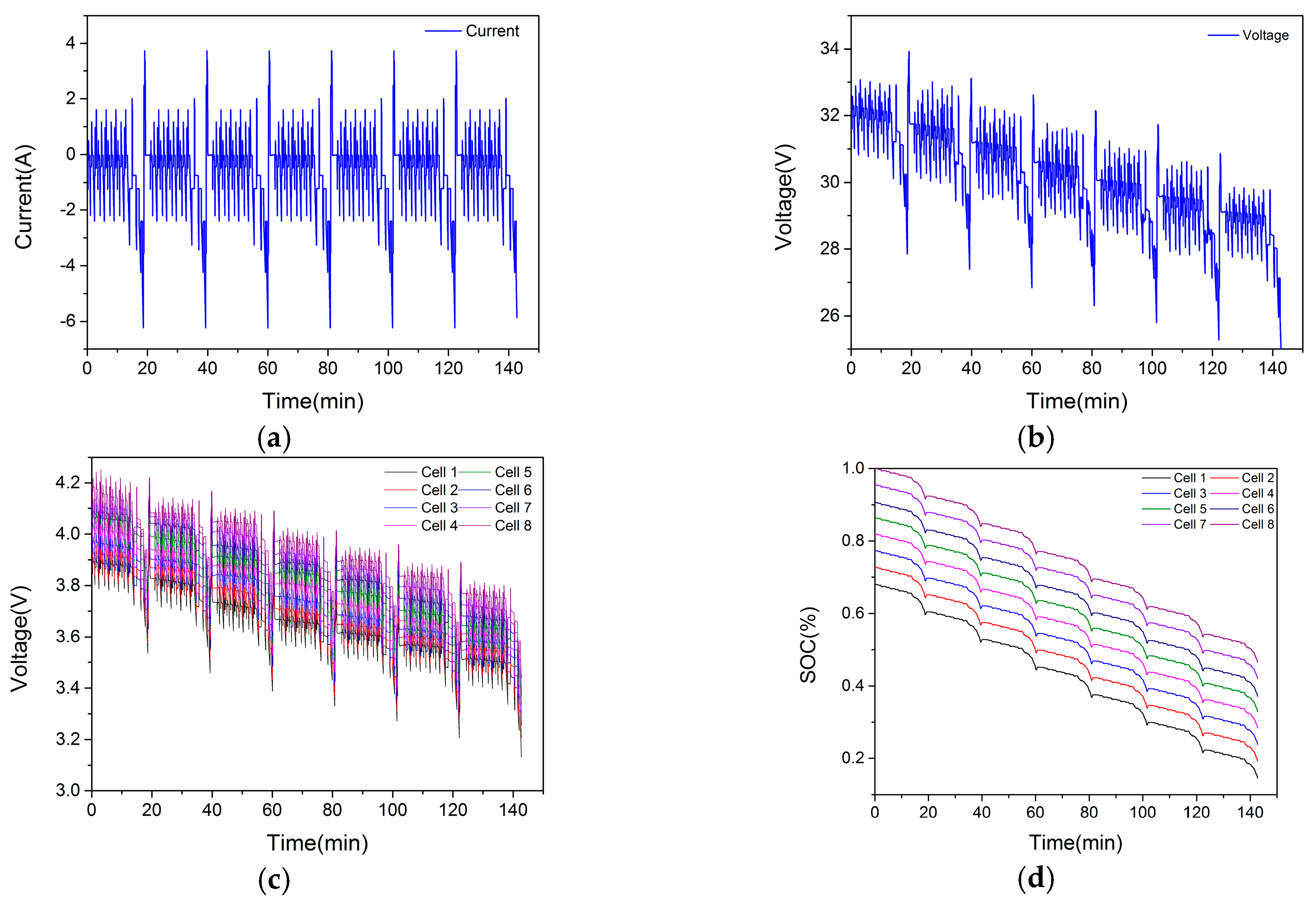
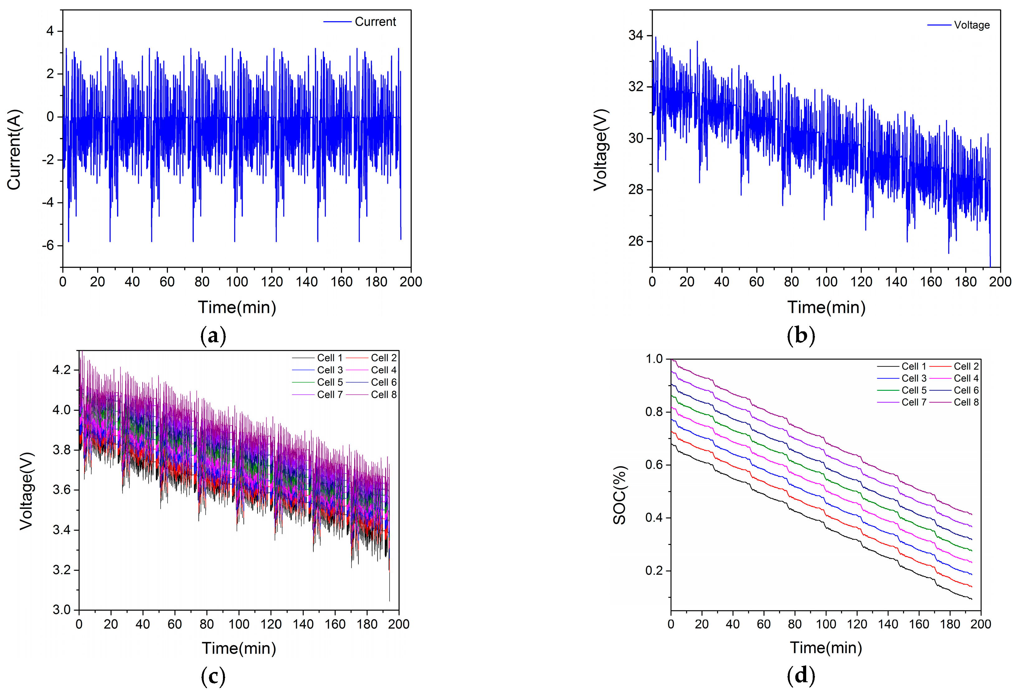
The battery module was conducted under the NEDC and UDDS dynamic power conditions, respectively. The current profile and terminal voltage of battery module under the NEDC condition is shown in Figure 7a,b. The terminal voltage and actual SOC value of each cell is shown in Figure 7c,d. The current profile and terminal voltage of the battery module under the UDDS condition is shown in Figure 8a,b. The terminal voltage and actual SOC value of each cell is shown in Figure 8c,d. The sampling period of all data was 0.1 s.

5. Results and Discussion

5.1. Battery Cell Calibration Results

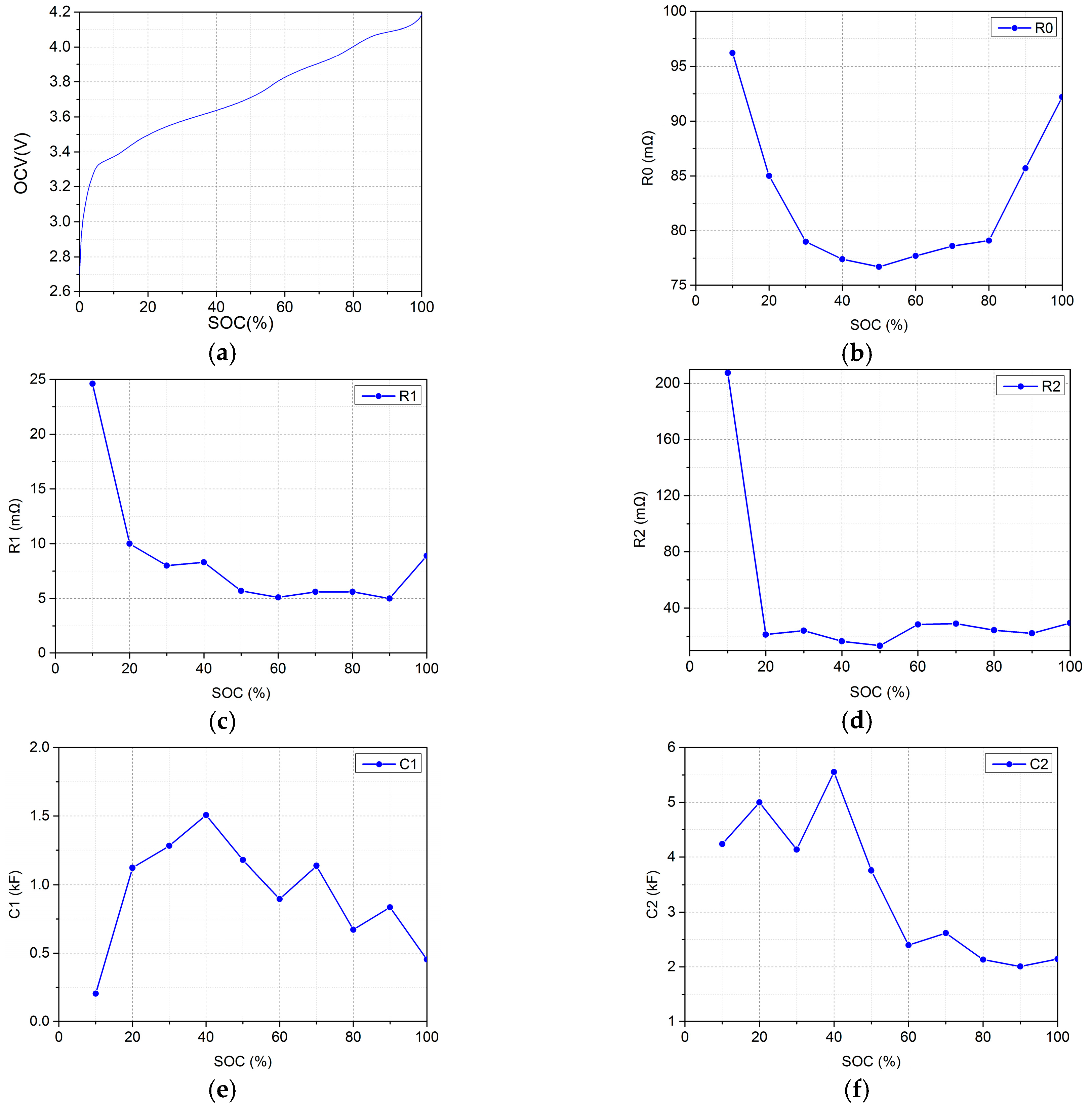
The calibrated SOC-OCV and SOC-parameters curve results of the specific cell are shown in Figure 9.

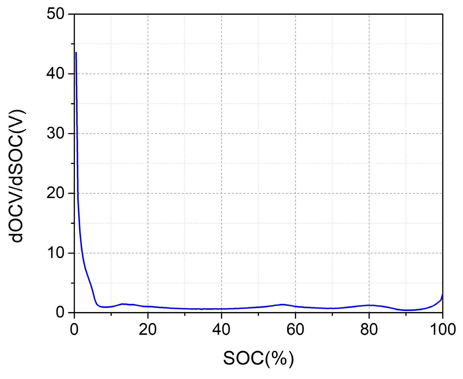
Figure 9a is the calibrated SOC-OCV curve. In the EKF algorithm, the dOCV-dSOC relationship is used. Considering that the SOC-OCV curve used in this paper was connected by the points in the interval of the 0.5% SOC, the same look-up table was established as the interpolation reference according to the 0.5% SOC segment, and the curve is shown in Figure 10.

5.2. Battery Pack SOC and R₀ Estimation Method Verification and Discussion

In this section, using the current and cell voltage data collected under the NEDC and UDDS conditions, the DTSDEKF algorithm introduced in Section 3.1 was utilized to estimate the SOC and R₀ of each cell based on the S&D battery pack model. The estimated SOC of each cell was compared with the actual SOC value to verify the SOC estimation accuracy. The estimated cell voltage was compared to the measured cell voltage to verify the R₀ estimation accuracy. The results under two conditions both verify the effectiveness of the DTSDEKF algorithm for state estimation of a battery pack. To better illustrate the effectiveness of the S&D model for battery pack state estimation, the same analysis was performed based on the commonly used M&D model. The results estimated by the two models were compared, and the difference between the two models was theoretically analyzed.

5.2.1. Battery Pack SOC and R₀ Estimation Result

The first step of the DTSDEKF algorithm using the S&D model is to select a specific cell. According to the analysis, theoretically, any cell can be selected. In the process of RDE estimation, the cell with the lowest initial voltage is selected as the specific cell; that is, cell 1. The process of the DTSDEKF algorithm using the M&D model is similar to that using the S&D model. It is only necessary to replace the specific cell with a virtual mean cell. The terminal voltage value of the mean cell is the average value of all the cell voltages.

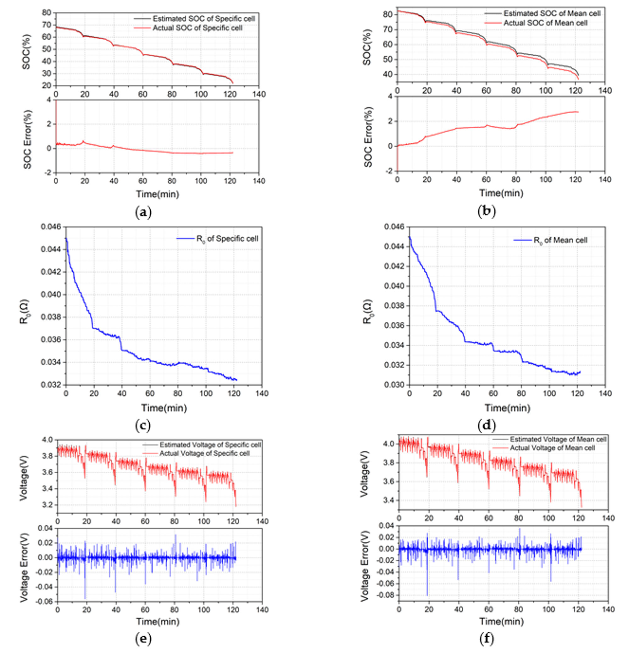
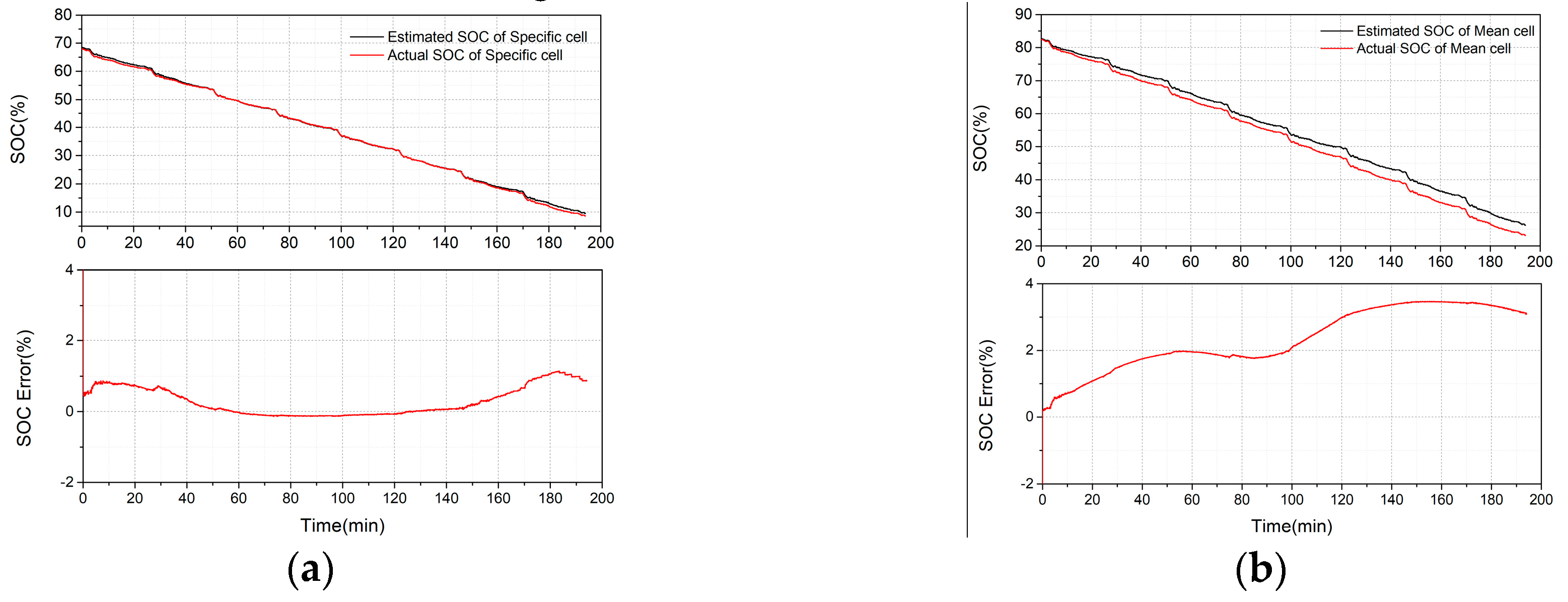
In the first time scale, the SOC and R₀ values of the specific cell in the S&D model and the mean cell in the M&D model are obtained. Figure 11a,b show the comparison between the estimated SOC result and the actual SOC and the estimation error of the specific cell and the mean cell, respectively. Figure 11c,d show the estimated R₀ result of the specific cell and mean cell. Figure 11e,f show the comparison between the estimated terminal voltage and the actual terminal voltage and the estimation error of the specific cell and the mean cell, respectively. It can be seen from the result that the estimated R₀ value and the terminal voltage error of the two algorithms are not much different, and both can accurately estimate the terminal voltage. However, the difference is that the SOC estimation error of the specific cell converges rapidly from 12% to less than 1%, and approaches zero as time increases, while the SOC estimation error of the mean cell diverges to around 3%.

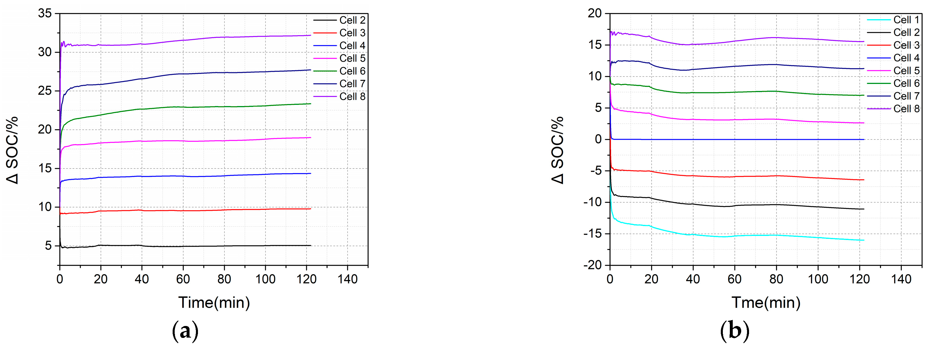
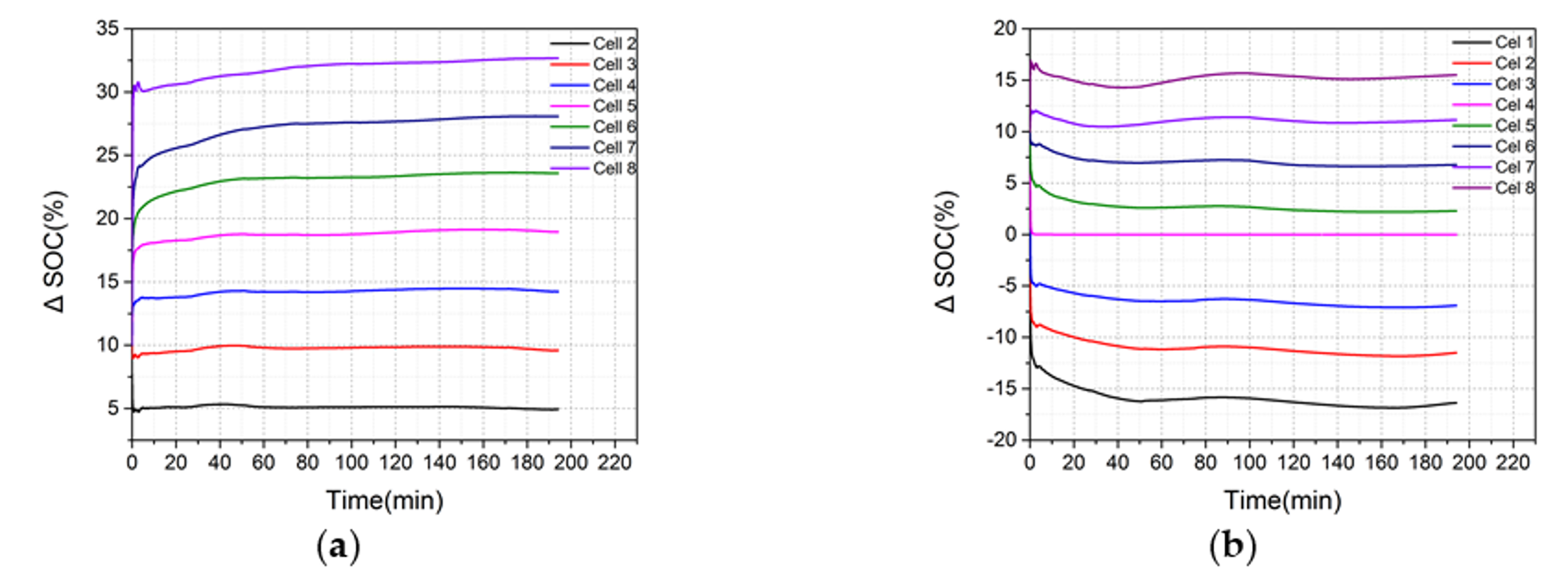
In the second time scale, the results of the ΔSOC between the other seven cells and the specific cell in the S&D model and the ΔSOC between the eight cells and the mean cell in the M&D model were obtained, as shown in Figure 12a,b respectively. The initial values of ΔSOC of the seven cells in the S&D model and the eight cells in the M&D model were all set to 10%. In the S&D model, since the actual ΔSOC of cell 3 is the closest to 10%, the estimated ΔSOC of it converges first. Similarly, the initial ΔSOC of cell 6 in the M&D model is the closest to 10% and it converges first, and cell 1 is the last to converge. However, after a few minutes of operation, the ΔSOC of the S&D model tends to be stable, while the results in the M&D model still slowly change. In general, the ΔSOC curve using the M&D model is not as stable as the curve using the S&D model.

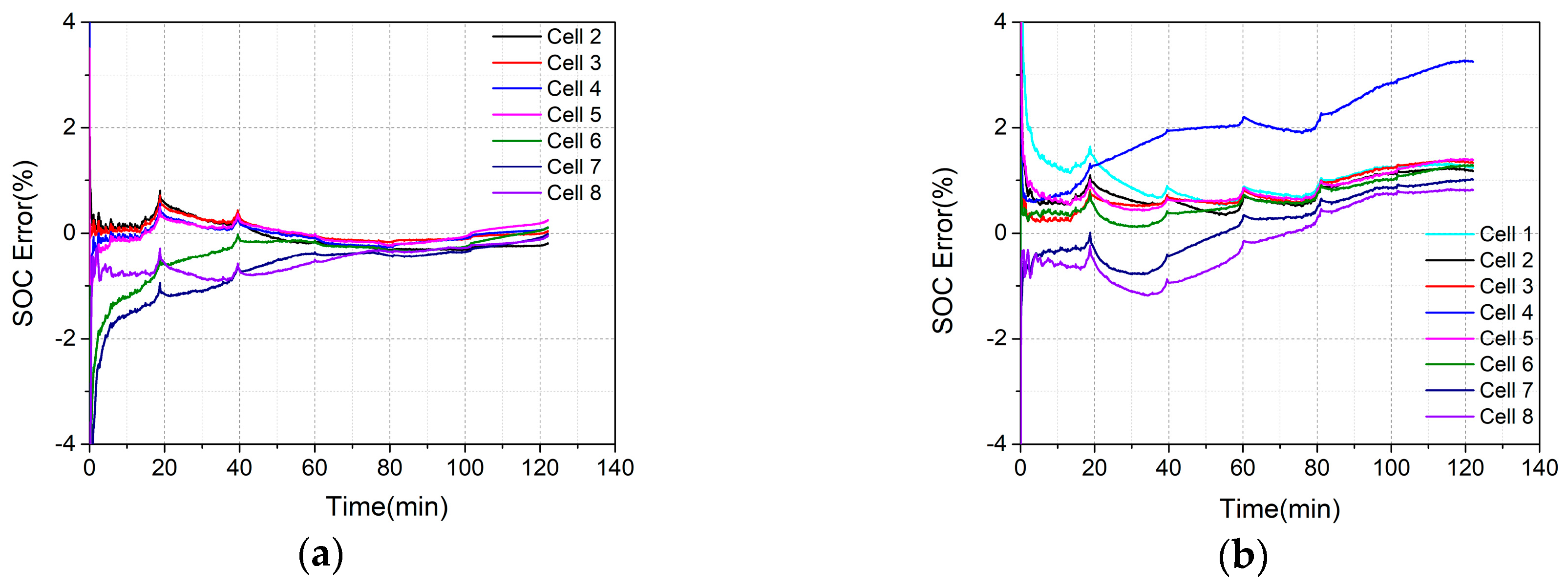
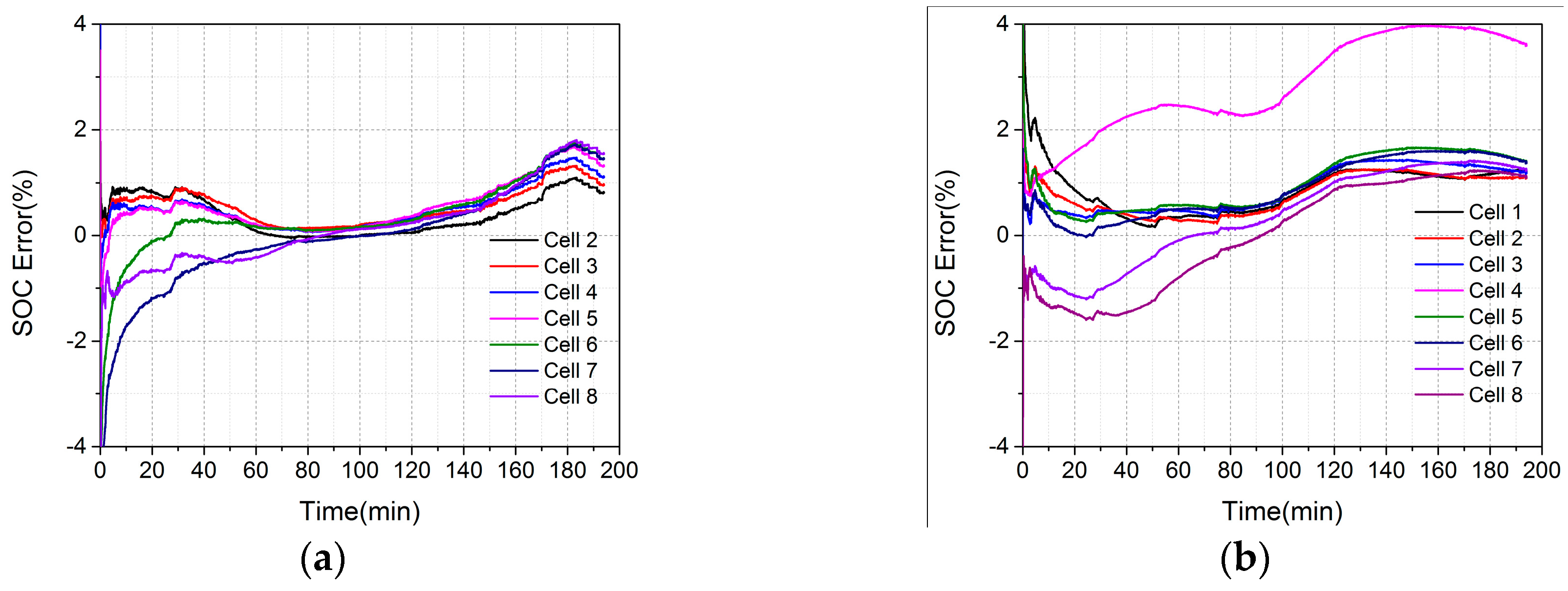
Figure 13a,b compare the SOC estimation error of each cell in the two models. When the S&D model is used, the SOC error of each cell is less than 1% for most of the time and finally converges to around 0%. When the M&D model is used, the error of cell 4 diverges to around 3%, while the other cell’s errors are eventually around 1%.

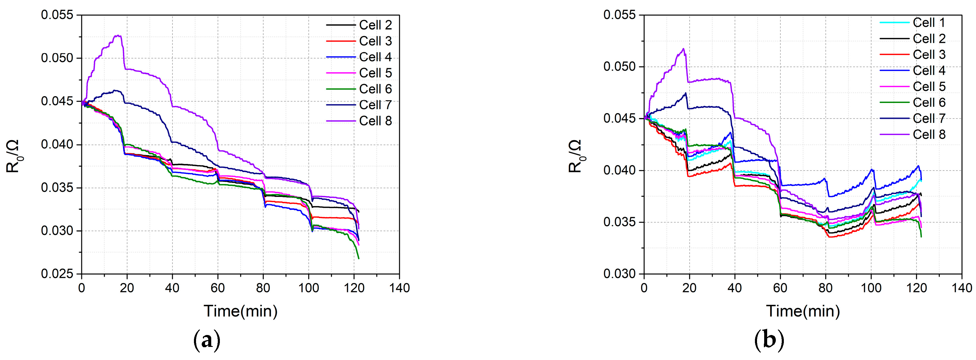
Figure 14a,b show the R₀ estimation results of the two models. Obviously, it can be seen that the variation in the S&D model is also smoother than that in the M&D model.

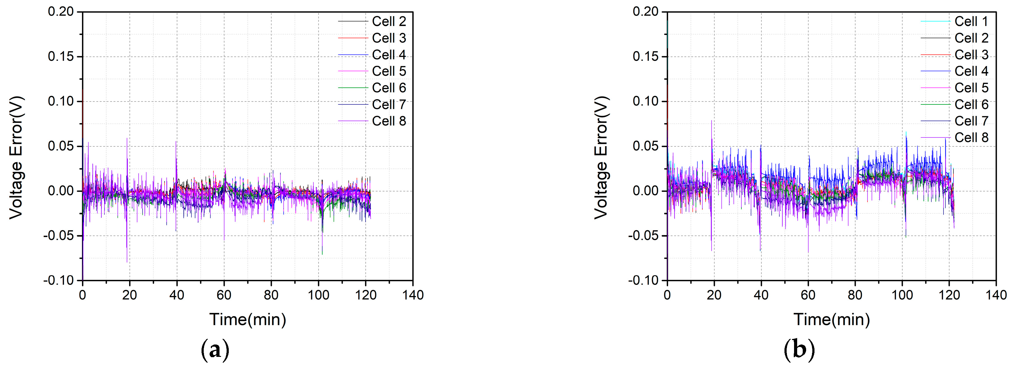
Moreover, the average value of the seven cells’ RMSE of the voltage error is 7.6 mV, and the value in the M&D model is 14.2 mV. Additionally, the comparison of the estimation error of the cells’ terminal voltage in Figure 15 shows that the S&D model is also smoother than the M&D model.

The same analysis was performed under the UDDS condition. According to the result under the NEDC condition, the main difference between the S&D and M&D model is mainly reflected in the estimation of each cell’s SOC within the battery pack. The results of the SOC estimation under the UDDS condition are shown in Figure 16, Figure 17 and Figure 18.

As can be seen from the results, the SOC estimation effect of each cell under the UDDS condition is similar to that under the NEDC condition, and the result also shows that the effect of the S&D model is better than that of the M&D model. Specifically, the SOC estimation result for the specific cell is within 1% during most of the entire discharge process, while that of the M&D model slowly increases to above 2% during most of the discharge process and diverges to around 4%. As for the SOC estimation effect of the other cells, the S&D model also shows a better performance. In the S&D model, the SOC error of the other cells remains within 1% during most of the discharge process, while that of the other cells in the M&D diverges to around 2% and the result of cell 4 is similar to that of the mean cell, which diverges to around 4%.

Therefore, from an experimental point of view, the SOC and R₀ estimation accuracy of the method using the S&D model and the DTSDEKF algorithm is verified, and it can be seen that the S&D model is better than the M&D model.

5.2.2. Analysis of the Difference between the S&D and M&D Model

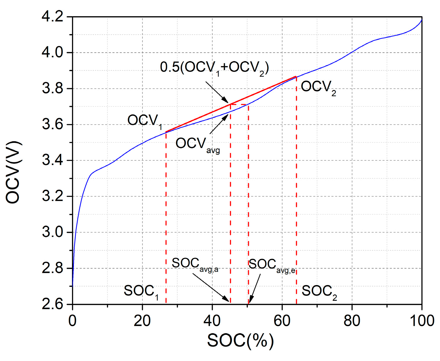
The main reason for the difference between the S&D model and the M&D model in estimating the SOC and terminal voltage of the battery cell lies in the characteristics of the SOC-OCV curve of the research subject. The SOC-OCV curve of the lithium iron phosphate (LFP) battery calibrated in [35] is basically straight in the SOC = 20%–70% segment, and the OCV change is only 0.3 V. The SOC value of the cell used in that experiment is in the range of 15% to 70%, and the average OCV value corresponding to the SOC state of the mean model is substantially equal to the average of the OCV values of the respective cells. While from the SOC-OCV curve of the NCA battery used in this research, it can be seen that the nonlinearity of the curve is relatively serious, and the OCV change is more severe. Taking two cells as an example, as shown in Figure 19, the SOC of the mean cell in the M&D model is estimated by using the average terminal voltage of two cells as the output, ignoring the influence of the polarization voltage; that is, the average OCV is 0.5*(OCV₁ + OCV₂), and the corresponding estimated SOC value is SOC_avg,e. While the actual SOC value of the mean cell is the average SOC value of the two cells, which is SOC_avg,a. The result is that the estimated SOC value is difficult to converge to the actual value, and the concept of the average SOC is hard to define and has no practical meaning. Therefore, the M&D model is not suitable for the state estimation of the pack using the batteries with a highly nonlinear SOC-OCV curve, such as the NCA battery used in this research, especially when the SOC difference between the cells is large.

5.2.3. Battery Pack RDE Prediction Method Verification

After estimating the present SOC and R₀ value of each cell, the next step is to determine the future SOC sequence according to the given future operating condition. Then, the future terminal voltage of each cell is predicted by the model parameters and R₀ prediction. The terminal voltage, current, and time of each cell are integrated to the RDE of the total RDE of the battery pack.

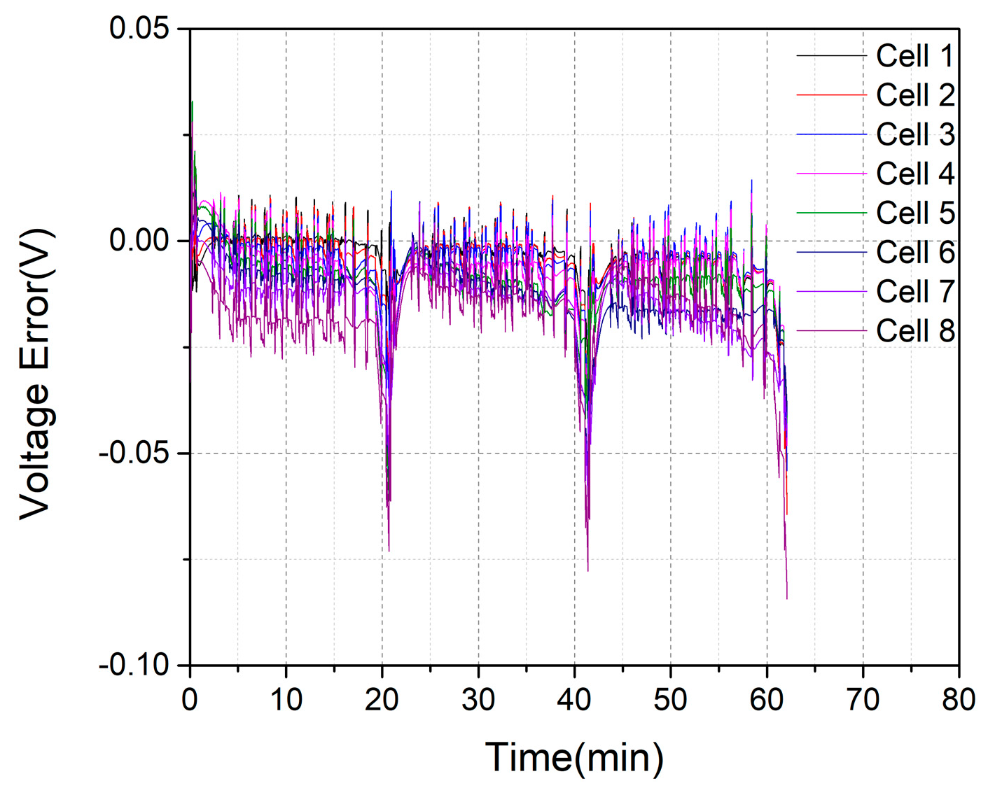
Take the NEDC condition as an example. The 60th minute is selected as the starting point of the prediction. Due to the inconsistency of SOC, the parameters of the RC parameters determined by the interpolation are inconsistent, so the prediction of the polarization voltage is also inconsistent. The error curves for the terminal voltage predictions of each cell are shown in Figure 20.

From the prediction error of the terminal voltage, the errors of cell 8 are also the largest. The reason is that the error of the SOC estimation is larger than the other cells, which causes the terminal voltage error to be higher than the other cells.

The final estimated RDE value is 18.8839 Wh, and the actual RDE value obtained by calculating the collected current, voltage value, and time is 18.8846 Wh. It can be seen that the estimation error is very small.

Table 5. Battery pack RDE prediction results at different starting points under the NEDC condition.

Starting Point	Predicted RDE (Wh)	Actual RDE (Wh)
20 min	31.7150	31.7163
40 min	25.4025	25.4035
60 min	18.8839	18.8846
80 min	13.8488	13.8493
100 min	8.6216	8.6220
120 min	2.7272	2.7273

lists the predicted RDE values versus the actual RDE values with the energy prediction algorithm, which selects the 20th, 40th, 60th, 80th, 100th, and 120th minute as the starting point, respectively. It can be seen that the proposed RDE prediction algorithm of the battery pack has very high precision, and all the errors are below 1%.

5.2.4. Limitations and Future Work

In this research, we only verified the accuracy of state estimation and the RDE prediction algorithm at room temperature, that is, 25 °C. Future research will focus on the verification at high and low temperatures and conditions where temperature inconsistency exists in the battery pack.

6. Conclusions

In this paper, for a batch of nickel cobalt aluminum oxide lithium-ion batteries, after analyzing the characteristics of battery model parameter inconsistency, a battery pack specific and difference model considering state of charge and R₀ inconsistency was established. Based on the model, the dual time-scale dual extended Kalman filter algorithm was proposed to estimate the state of charge and R₀ of each cell in the battery pack, and the remaining discharge energy prediction algorithm of the battery pack was established based on the state estimation results.

Under the NEDC and UDDS condition, the effectiveness of the state estimation and the remaining discharge energy prediction algorithm was verified. The results show that the state of charge estimation error of each cell is less than 1%, and the convergence speed is fast. The remaining discharge energy prediction error of the battery pack is less than 1% over the entire discharge cycle. Besides, the difference between the specific and difference and mean and difference models was also analyzed. The main reason that causes the difference between the two is the nonlinearity of the SOC-OCV curve of the battery used. When the nonlinearity of the SOC-OCV curve is serious, such as the nickel cobalt aluminum oxide cell used in this research, the specific and difference model has higher precision.

References

- Neubauer, J.; Wood, E. The impact of range anxiety and home, workplace, and public charging infrastructure on simulated battery electric vehicle lifetime utility. J. Power Sources 2014, 257, 12–20. [Google Scholar] [CrossRef]
- Liu, X.T.; Wu, J.; Zhang, C.B.; Chen, Z.H. A method for state of energy estimation of lithium-ion batteries at dynamic currents and temperatures. J. Power Sources 2014, 270, 151–157. [Google Scholar] [CrossRef]
- Bingham, C.; Walsh, C.; Carroll, S. Impact of driving characteristics on electric vehicle energy consumption and range. IET Intell. Transp. Syst. 2012, 6, 29–35. [Google Scholar] [CrossRef]
- Gong, Q.M.; Li, Y.Y.; Peng, Z.R. Trip based optimal power management of plug-in hybrid electric vehicles using gas-kinetic traffic flow model. In Proceedings of the 2008 American Control Conference, Seattle, WA, USA, 11–13 June 2008. [Google Scholar]
- Mamadou, K.; Lemaire, E.; Delaille, A.; Riu, D.; Hing, S.E.; Bultel, Y. Definition of a State-of-Energy Indicator (SoE) for Electrochemical Storage Devices: Application for Energetic Availability Forecasting. J. Electrochem. Soc. 2012, 159, A1298–A1307. [Google Scholar] [CrossRef]
- Wang, Y.J.; Zhang, C.B.; Chen, Z.H. An adaptive remaining energy prediction approach for lithium-ion batteries in electric vehicles. J. Power Sources 2016, 305, 80–88. [Google Scholar] [CrossRef]
- Zhang, W.G.; Shi, W.; Ma, Z.Y. Adaptive unscented Kalman filter based state of energy and power capability estimation approach for lithium-ion battery. J. Power Sources 2015, 289, 50–62. [Google Scholar] [CrossRef]
- He, H.W.; Zhang, Y.Z.; Xiong, R.; Wang, C. A novel Gaussian model based battery state estimation approach: State-of-Energy. Appl. Energy 2015, 151, 41–48. [Google Scholar] [CrossRef]
- Zheng, L.F.; Zhu, J.G.; Wang, G.X.; He, T.T.; Wei, Y.Y. Novel methods for estimating lithium-ion battery state of energy and maximum available energy. Appl. Energy 2016, 178, 1–8. [Google Scholar] [CrossRef]
- Ceraolo, M.; Pede, G. Techniques for estimating the residual range of an electric vehicle. IEEE Trans. Veh. Technol. 2001, 50, 109–115. [Google Scholar] [CrossRef]
- Liu, G.M.; Ouyang, M.G.; Lu, L.G.; Li, J.Q.; Hua, J.F. A highly accurate predictive-adaptive method for lithium-ion battery remaining discharge energy prediction in electric vehicle applications. Appl. Energy 2015, 149, 297–314. [Google Scholar] [CrossRef]
- Hannan, M.A.; Lipu, M.S.H.; Hussain, A.; Mohamed, A. A review of lithium-ion battery state of charge estimation and management system in electric vehicle applications: Challenges and recommendations. Renew. Sust. Energ. Rev. 2017, 78, 834–854. [Google Scholar] [CrossRef]
- Hu, X.S.; Li, S.B.; Peng, H. A comparative study of equivalent circuit models for Li-ion batteries. J. Power Sources 2012, 198, 359–367. [Google Scholar] [CrossRef]
- Xiong, R.; Sun, F.C.; Gong, X.Z.; Gao, C.C. A data-driven based adaptive state of charge estimator of lithium-ion polymer battery used in electric vehicles. Appl. Energy 2014, 113, 1421–1433. [Google Scholar] [CrossRef]
- Zheng, Y.J.; Han, X.B.; Lu, L.G.; Li, J.Q.; Ouyang, M.G. Lithium ion battery pack power fade fault identification based on Shannon entropy in electric vehicles. J. Power Sources 2013, 223, 136–146. [Google Scholar] [CrossRef]
- Prasad, G.K.; Rahn, C.D. Model based identification of aging parameters in lithium ion batteries. J. Power Sources 2013, 232, 79–85. [Google Scholar] [CrossRef]
- Ouyang, M.G.; Liu, G.M.; Lu, L.G.; Li, J.Q.; Han, X.B. Enhancing the estimation accuracy in low state-of-charge area: A novel onboard battery model through surface state of charge determination. J. Power Sources 2014, 270, 221–237. [Google Scholar] [CrossRef]
- Yang, M.L.; Zhang, X.H.; Li, X.H.; Wu, X.Z. A hybrid genetic algorithm for the fitting of models to electrochemical impedance data. J. Electroanal. Chem. 2002, 519, 1–8. [Google Scholar] [CrossRef]
- Lin, C.; Mu, H.; Xiong, R.; Shen, W.X. A novel multi-model probability battery state of charge estimation approach for electric vehicles using H-infinity algorithm. Appl. Energy 2016, 166, 76–83. [Google Scholar] [CrossRef]
- Chen, Z.; Mi, C.C.; Fu, Y.H.; Xu, J.; Gong, X.Z. Online battery state of health estimation based on Genetic Algorithm for electric and hybrid vehicle applications. J. Power Sources 2013, 240, 184–192. [Google Scholar] [CrossRef]
- Zhang, X.; Wang, Y.J.; Liu, C.; Chen, Z.H. A novel approach of battery pack state of health estimation using artificial intelligence optimization algorithm. J. Power Sources 2018, 376, 191–199. [Google Scholar] [CrossRef]
- Plett, G.L. Recursive approximate weighted total least squares estimation of battery cell total capacity. J. Power Sources 2011, 196, 2319–2331. [Google Scholar] [CrossRef]
- Zahid, T.; Li, W.M. A Comparative Study Based on the Least Square Parameter Identification Method for State of Charge Estimation of a LiFePO4 Battery Pack Using Three Model-Based Algorithms for Electric Vehicles. Energies 2016, 9, 16. [Google Scholar] [CrossRef]
- Plett, G.L. Extended Kalman filtering for battery management systems of LiPB-based HEV battery packs: Part 3. State and parameter estimation. J. Power Sources 2004, 134, 277–292. [Google Scholar] [CrossRef]
- Xiong, R.; Sun, F.C.; He, H.W.; Nguyen, T.D. A data-driven adaptive state of charge and power capability joint estimator of lithium-ion polymer battery used in electric vehicles. Energy 2013, 63, 295–308. [Google Scholar] [CrossRef]
- Hu, X.S.; Sun, F.C.; Zou, Y.A. Estimation of State of Charge of a Lithium-Ion Battery Pack for Electric Vehicles Using an Adaptive Luenberger Observer. Energies 2010, 3, 1586–1603. [Google Scholar] [CrossRef]
- Chen, Z.; Li, X.Y.; Shen, J.W.; Yan, W.S.; Xiao, R.X. A Novel State of Charge Estimation Algorithm for Lithium-Ion Battery Packs of Electric Vehicles. Energies 2016, 9, 15. [Google Scholar] [CrossRef]
- Xu, L.; Wang, J.P.; Chen, Q.S. Kalman filtering state of charge estimation for battery management system based on a stochastic fuzzy neural network battery model. Energy Conv. Manag. 2012, 53, 33–39. [Google Scholar] [CrossRef]
- Dai, H.F.; Guo, P.J.; Wei, X.Z.; Sun, Z.C.; Wang, J.Y. ANFIS (adaptive neuro-fuzzy inference system) based online SOC (State of Charge) correction considering cell divergence for the EV (electric vehicle) traction batteries. Energy 2015, 80, 350–360. [Google Scholar] [CrossRef]
- Ouyang, M.G.; Zhang, M.X.; Feng, X.N.; Lu, L.G.; Li, J.Q.; He, X.M.; Zheng, Y.J. Internal short circuit detection for battery pack using equivalent parameter and consistency method. J. Power Sources 2015, 294, 272–283. [Google Scholar] [CrossRef]
- Zheng, Y.J.; Ouyang, M.G.; Lu, L.G.; Li, J.Q. Understanding aging mechanisms in lithium-ion battery packs: From cell capacity loss to pack capacity evolution. J. Power Sources 2015, 278, 287–295. [Google Scholar] [CrossRef]
- Chiu, K.C.; Lin, C.H.; Yeh, S.F.; Lin, Y.H.; Huang, C.S.; Chen, K.C. Cycle life analysis of series connected lithium-ion batteries with temperature difference. J. Power Sources 2014, 263, 75–84. [Google Scholar] [CrossRef]
- Yang, N.X.; Zhang, X.W.; Shang, B.B.; Li, G.J. Unbalanced discharging and aging due to temperature differences among the cells in a lithium-ion battery pack with parallel combination. J. Power Sources 2016, 306, 733–741. [Google Scholar] [CrossRef]
- Sepasi, S.; Roose, L.R.; Matsuura, M.M. Extended Kalman Filter with a Fuzzy Method for Accurate Battery Pack State of Charge Estimation. Energies 2015, 8, 5217–5233. [Google Scholar] [CrossRef]
- Zheng, Y.J.; Ouyang, M.G.; Lu, L.G.; Li, J.Q.; Han, X.B.; Xu, L.F.; Ma, H.B.; Dollmeyer, T.A.; Freyermuth, V. Cell state-of-charge inconsistency estimation for LiFePO4 battery pack in hybrid electric vehicles using mean-difference model. Appl. Energy 2013, 111, 571–580. [Google Scholar] [CrossRef]
- Dai, H.F.; Wei, X.Z.; Sun, Z.C.; Wang, J.Y.; Gu, W.J. Online cell SOC estimation of Li-ion battery packs using a dual time-scale Kalman filtering for EV applications. Appl. Energy 2012, 95, 227–237. [Google Scholar] [CrossRef]
- Waag, W.; Kabitz, S.; Sauer, D.U. Experimental investigation of the lithium-ion battery impedance characteristic at various conditions and aging states and its influence on the application. Appl. Energy 2013, 102, 885–897. [Google Scholar] [CrossRef]
- Boukamp, B.A. Electrochemical impedance spectroscopy in solid state ionics: recent advances. Solid State Ion. 2004, 169, 65–73. [Google Scholar] [CrossRef]
Figure 1.
Schematic diagram of remaining discharge energy.
Figure 2.
Schematic diagram of second-order ECM.
Figure 3.
ECM of a serial-connected battery pack.
Figure 4.
Impedance spectra of 40 cells at 25 °C, 50% SOC. (a) The original results; (b) the results after translation.
Figure 5.
Flow chart of the dual time-scale dual EKF algorithm.
Figure 6.
Profile of the HPPC condition.
Figure 7.
NEDC profile. (a) The current profile; (b) the terminal voltage of the battery module; (c) the terminal voltage of each cell; (d) the actual SOC value of each cell.
Figure 8.
UDDS profile. (a) The current profile; (b) the terminal voltage of the battery module; (c) the terminal voltage of each cell; (d) the actual SOC value of each cell.
Figure 9.
Calibrated results for cell. (a) SOC-OCV curve; (b) SOC-R0 curve; (c) SOC-R1 curve; (d) SOC-R2 curve; (e) SOC-C1 curve; (f) SOC-C2 curve.
Figure 10.
dOCV-dSOC curve.
Figure 11.
Results of the specific cell and the mean cell under the NEDC condition. (a) SOC estimation result of the specific cell; (b) SOC estimation result of the mean cell; (c) R0 estimation result of the specific cell; (d) R0 estimation result of the mean cell; (e) terminal voltage estimation result of the specific cell; (f) terminal voltage estimation result of the mean cell.
Figure 12.
Results of the ΔSOC under the NEDC condition. (a) ΔSOC results of the S&D model; (b) ΔSOC results of the M&D model.
Figure 13.
Results of each cell’s SOC estimation error under the NEDC condition. (a) S&D model; (b) M&D model.
Figure 14.
Results of each cell’s R0 estimation under the NEDC condition. (a) S&D model; (b) M&D model.
Figure 15.
Results of each cell’s voltage estimation error under the NEDC condition. (a) S&D model; (b) M&D model.
Figure 16.
Results of the specific cell and the mean cell under the UDDS condition. (a) SOC estimation result of the specific cell; (b) SOC estimation result of the mean cell.
Figure 17.
Results of the ΔSOC under the UDDS condition. (a) ΔSOC results of the S&D model; (b) ΔSOC results of the M&D model.
Figure 18.
Results of each cell’s SOC estimation error under UDDS condition. (a) S&D model; (b) M&D model.
Figure 19.
Analysis of the S&D and M&D model difference on the SOC–OCV curve.
Figure 20.
Voltage prediction error of each cell under the NEDC condition.