HyFlow—A Hybrid Load Flow-Modelling Framework to Evaluate the Effects of Energy Storage and Sector Coupling on the Electrical Load Flows

Abstract

HyFlow is a grid-based multi-energy system (MES) modelling framework. It aims to model the status quo of current energy systems, future scenarios with a high share of fluctuating energy sources or additional consumers like electric vehicles, and to compare solution strategies if certain parts of the infrastructure are congested. In order to evaluate the congestion limits and the feasibility and suitability of solution strategies (e.g., energy storage, sector coupling technologies, demand response (DR)), load flow calculations of all three main grid-bound energy carriers are implemented in one single modelling framework. In addition to the implemented load flow models, it allows the interaction of these grids with the use of hybrid elements. This measure enables a proper assessment of future scenarios, not only for the infrastructure of one energy carrier, but for the overall energy system. The calculation workflow of HyFlow, including the implemented load flow calculations, as well as the implementation of the flexibility options, is described in detail in the methodology section. To demonstrate the wide range of applicability of HyFlow with different spatial ranges, two case studies referring to current research problems are presented: a city and a region surrounding the mentioned city. The calculations for the mentioned case studies are performed for three levels. A “status quo” level, a “high-stress” level with added fluctuating energy sources and consumers, and an “improvement” level, where flexibility options are introduced to the system. The effect of the flexibility options on future energy grids is, therefore, analyzed and evaluated. A wide variety of evaluation criteria can be selected. For example, the maximum load of certain power lines, the self-sufficiency of the overall system, the total transport losses or the total energy consumption.

1. Introduction

Energy production from renewable sources greatly fluctuates due to daily cycles, weather conditions and seasonal variation. This inevitably leads to situations with higher peaks in energy production and times of shortages. As a result, this volatility is expected to place stress on the grid. There are different means of managing this additional grid including curtailment measures in periods of high energy generation, grid expansion measures, energy storage installation, and sector coupling between different energy carriers. In order to evaluate these options, a load flow calculation is necessary for all grid-bound energy carriers; the modelling framework needs to be modular and flexible to deal with a wide range of possible spatial—and temporal resolutions; and all relevant mentioned elements in terms of storage of sector coupling need to be implemented. The HyFlow modelling framework introduced here aims to model the status quo of current energy systems and future scenarios with a high share of fluctuating energy sources or additional consumption, and to compare solution strategies if certain parts of the infrastructure are congested. This solution approach goes beyond current multi-energy system (MES) approaches, by considering all grid limitations of electricity-, natural gas and district heating networks. This allows the user a more detailed, holistic picture of cross-sectoral energy applications and the consequences for energy distribution.

2. State of Research in Modelling Multi-Energy Systems (MES)

The following section gives a brief overview of existing MES modelling approaches and their characteristics in order to classify the presented HyFlow approach into various categories and point out its advantages and disadvantages compared to other modelling frameworks. In order to compare HyFlow with other MES modelling approaches the main categories used to distinguish between types of MES modelling approaches are discussed.

Mancarella et al. [1] identify four main distinguishing features used to characterize MES modelling approaches: multi-fuel, multi-service, spatial resolution and network connections. Additionally, they argue that time resolution of MES should be considered as an additional distinguishing factor. These five factors seem suitable to classify the HyFlow modelling framework compared to other MES modelling approaches and will be further discussed in the next section. As the main focus of the system presented is on the spatial and time resolution, especially on the network connections, these features are discussed in more detail than the multi-fuel and multi-service perspective, which the HyFlow framework considers as well.

Multi-fuel means that the same final energy demand (e.g., domestic heat) can be supplied by different energy sources like district heating, a heat pump or a gas boiler. Multi-fuel approaches can be divided into full and hybrid approaches. While full approaches consider all available energy carriers, the hybrid approaches consider only the relevant energy carriers for the task. As the HyFlow modelling framework focuses on grid-bound energy supply, only three energy carriers are implemented (electricity, natural gas and district heat). Full approaches consider additional energy carriers like coal, uranium, kerosene or hydrogen as well.

The second mentioned differentiation characteristic is multi-service. A multi-service MES modelling approach can include energy supply appliances that supply more than one energy service from one energy carrier (e.g., CHP plants that produce heat and power from natural gas) at the same time. The combination of a multi-fuel and multi-service modelling approach allows a wide range of technical and economical comparisons to be addressed; for example, between different energy sources and demands like primary energy efficiency, specific CO₂ emissions or operational costs.

The time horizon and the temporal resolution are important factors to consider when designing an MES modelling tool. Planning tools or economic assessments tend to have longer time horizons (30–50 years) than technical models, which analyze operational conditions (day–year) [2,3]. Many models use time-aggregated data and time steps ranging from μs for certain research questions in electrical grids to months in the case of seasonal influences of integrating renewable energy sources (RES) [4] to years in strategic planning tools. All models that use time steps and a static approach assume that fast phenomena have reached equilibrium at the end of the time step used. It should be noted, that the selection of an appropriate time interval is critical as different time-steps can lead to deviations in the results [5,6,7]. MES modelling approaches that focus on the integration of RES, [8] recommend 15-min time-steps.

The spatial coverage and resolution describes the geographical scope and the defined system boundaries of the MES modelling approach. There is a variety of spatial resolutions used in MES modelling approaches: these range from high-resolution single buildings, which may be used to model residential demand [9] or in the design stage of buildings [10], to large regions or countries [11,12]. Most publications of MES modelling approaches, however, use a spatial resolution that falls between these two extremes, such as suburbs, districts, cities or smaller regions. This may be seen in [3,13,14]. The spatial coverage also has a significant effect on other characteristics of MES modelling approaches. In particular, the level of detail, the time horizon and the possible network calculations is usually decreased for larger spatial coverage and resolution due to the higher computational time needed [2,15]. Models covering more than a few buildings usually use a simplified and highly aggregated modelling approach [2]. The HyFlow modelling framework presented here is combined with a cellular approach (presented in Section 3) to be as versatile and generic in terms of spatial coverage and resolution as possible, allowing a high degree of accuracy in terms of the original situation. It can be used for a range from multiple buildings to large regions.

To transport energy from the location of supply to the location of demand, an energy transportation network is needed. Grid-bound MES may also be characterized by their network structure. Since HyFlow, as a modelling framework, focuses on network infrastructure, this point of characterization is of particular in this paper. The network interconnections may also be distinguished by their level of detail. The interconnections range from highly detailed load flow calculations based on real physical conditions, to no restrictions or losses for the transport of energy at all. Geidl et al. [16] suggest a differentiation between power flow models and network models. The latter can be further divided into type 1 and type 2 network models, which are both highly simplified. Type 1 models (also referred as copper plate approach or single node model) feature flows that transport energy without experiencing losses, while type 2 models (transshipment model) consider energy losses as a function of the corresponding flow [17]. In MES modelling approaches that use the type 2 network calculations, no differentiation between energy carriers is necessary. By contrast, power flow models are based on physical principles like conservation laws and are the most accurate. Since the applied physical laws such as the relation between electric voltage and current, or hydraulic pressure and mass flow differ among the modelled energy carriers, no general model is applicable to all grid types [16]. There are calculation tools for each grid type, which are dedicated to static load flow calculations based on physical principles. Examples for the electricity sector are DIgSILENT PowerFactory [18], PSS Sincal [19] or Neplan [20], while the latter two can also be used for calculations concerning the gas and district heating grids. It is important to remark that none of these tools are able to interconnect the mentioned energy carriers. Further distinctions between different types of power flow calculations for electricity, gas and district heating networks are discussed in next section.

2.1. Electrical Network

There are two kinds of power flow models that are widely used in electrical grid representations—the direct current (DC) and the alternating current (AC) power flow model. In the DC model, nodes are determined and connected via lines. Kirchhoff’s law may then be used to calculate power flows based on the maximum power and corresponding line resistances. The AC power flow model furthermore considers the capacitive and inductive behavior of the grid and load. It is the most precise model, because it can additionally describe the reactive power in the system. However, additional parameters in the system need to be defined (e.g., iron losses in transformers, gear ratio or the phase shift) if more than one voltage level needs to be modelled [17,21]. There are several papers addressing the accuracy and the differences of results using a DC and an AC power flow approach. [22,23,24] The increased level of detail adds to the complexity of the system and prevents the AC model from being widely used in large scale MES modelling approaches [25] due to high computational times [17,22]. The AC power flow approach is, therefore, predominantly used in high-precision calculations of utilities.

The presented HyFlow modelling framework uses a DC power flow model and an adoption of it, because the first two network models (single node model and transshipment model) did not meet all the set requirements. The computational time and necessary amount of data for the AC power flow model was also considered to be too high.

Additionally, it is worth mentioning, that there are different approaches for power flow modelling independently from the load flow calculation process itself. One distinguishes between deterministic load flow (DLF) and probabilistic load flow (PLF) calculations. While the values of the load and the energy generation must be known for all nodes at the DLF, the PLF calculation considers stochastic variations of loads and generation. This is especially advantageous for modelling a small number of loads with a low simultaneity factor and renewable generation profiles, which are subject to greater fluctuations. The implementation of the uncertainty takes place via probability density functions for loads and fluctuating generation. Examples for the implementation of PLF calculations are to be found in commercial software (e.g., DigSilent) and scientific publications [26,27,28,29], especially often in combination with a Monte Carlo approach. HyFlow considers the DPF method with set values from the user. In the presented case studies, the load is modelled with an external stochastic approach [30], standard load profiles for highly aggregated applications with limited uncertainty and renewable generation based on measured historic data, which is subject to natural fluctuations.

2.2. Gas and District Heating Networks

The modelling of power flows in pipeline networks has a number of differences to the electrical grid. The biggest challenge is the non-linearity of the relationship between the power flow and the corresponding pressure loss. An additional difficulty for district heating grids only is considering the heat loss, which is decoupled from the power flow and only dependent on the temperature difference between the current fluid and the ambient temperature. This is aggravated by the fact that many material properties such as the kinematic viscosity or the density of fluids are dependent on the predominant nominal temperature and pressure levels. These various interactions add to the complexity of the system if they are not simplified or neglected. In the most practical models of pipeline networks, static approaches have been used and the non-linear dependency is solved either by linearization [31] or non-linear models [32,33]. In the HyFlow modelling framework, the quadratic dependency is solved by linearization. A more detailed explanation is given in the methodology in Section 4.3.2 of this paper.

In conclusion, there are separate load flow calculation tools, but according to [34] it is not possible to interconnect the energy carriers. Additionally Lund et al. and Pillai et al. [11,12] claim that studies with a higher spatial coverage and resolution usually do not account for system operation and infrastructure details. Kriechbaum et al. [34] conclude, that MES modelling approaches should incorporate the interactions between different energy carriers and models need to further include physical load flows in the implemented network connections. Tools that are capable of modelling physical load flows of the three grid-bound energy carriers and offer interconnections between them with hybrid elements do not exist. HyFlow addresses this precise gap and offers a solution to couple the load flow calculations.

3. Problem Definition and Solution Approach

The idea behind HyFlow is to have a tool that is able to model a wide range of energy systems. It should be able to solve tasks with one energy carrier as well as multiple energy carriers in microgrids, small local energy communities and large geographic regions, at a single time point and defined time-frames. The main driver for HyFlow is the increased share of fluctuating power supply in the electricity grid. Many sources state that an increased share of these decentralized generation technologies like solar or wind will need flexibility options in order to manage inevitable demand and supply mismatches at any given time. When modelling energy storage and hybrid elements it is quickly evident that the electricity grid cannot be the overall system border, although most of the RES like wind and photovoltaic (PV) power will be integrated into the electrical grid and implies big challenges for it [13,35]. An increased share of flexibility options such as storages and hybrid elements in the energy system also have large effects on other grids—especially the heat and natural gas grids. The consequence of this matter was a decision to create a modelling framework that is able to model the impacts on all three grids that are common at distribution level. The following bullet points summarize the main properties of HyFlow:

• Modelling of MES with three energy carriers (electricity, natural gas, heat);
• Large spatial range (households to large geographic regions);
• Flexible time framework (time interval and temporal resolution);
• Load flow calculations in all three modelled energy carriers and possible interactions between these grids via hybrid elements;
• Energy storage implementation (generic implementation—all technologies deployable);
• Hybrid element implementation (interconnections between energy carriers).

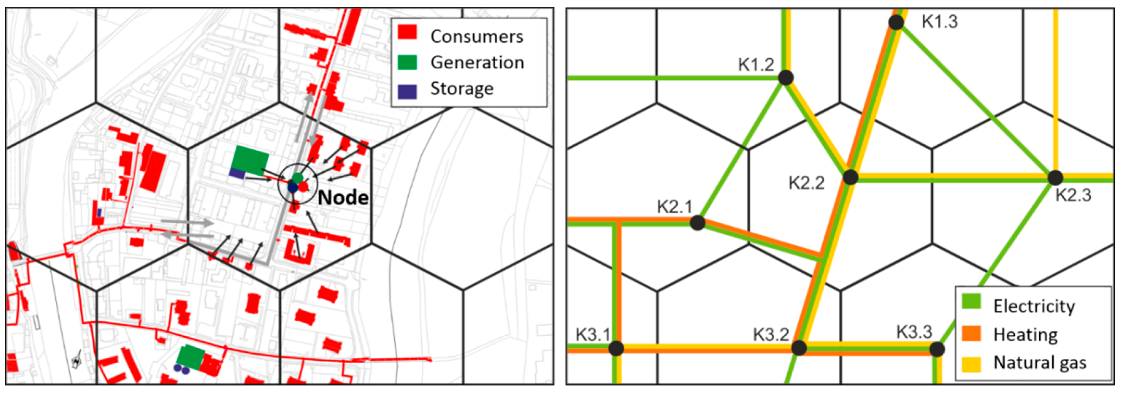
To set up a modelling framework with such a large spectrum of applications, the approach has to be as modular and generic as possible. An integrated framework, which plays a major role in HyFlow is the so-called “cellular approach”. The process of the cellular approach is visualized in Figure 1. All energy consumers, energy generation and energy storage units are aggregated to a single node within a defined cell or system boundary for every time step. This procedure is followed for every energy carrier. It is important to choose the cells according to geographical circumstances, the number of aggregated users, and the grid routes. More detailed recommendations regarding cell design within the cellular approach can be found in previous publications of Kienberger et al. [36,37].

The main objective of the cellular approach is to balance the supply and demand at the lowest possible level to prevent high load flows over the network connections. The implementation of the cellular approach in HyFlow is described in Section 4.1.

4. Methodology

This section shows how the objectives of the cellular approach are implemented in the HyFlow modelling framework. All of the important components and their characterization, as well as the implementation of the load flow calculations and the workflow of HyFlow are described.

4.1. Cellular Approach in HyFlow

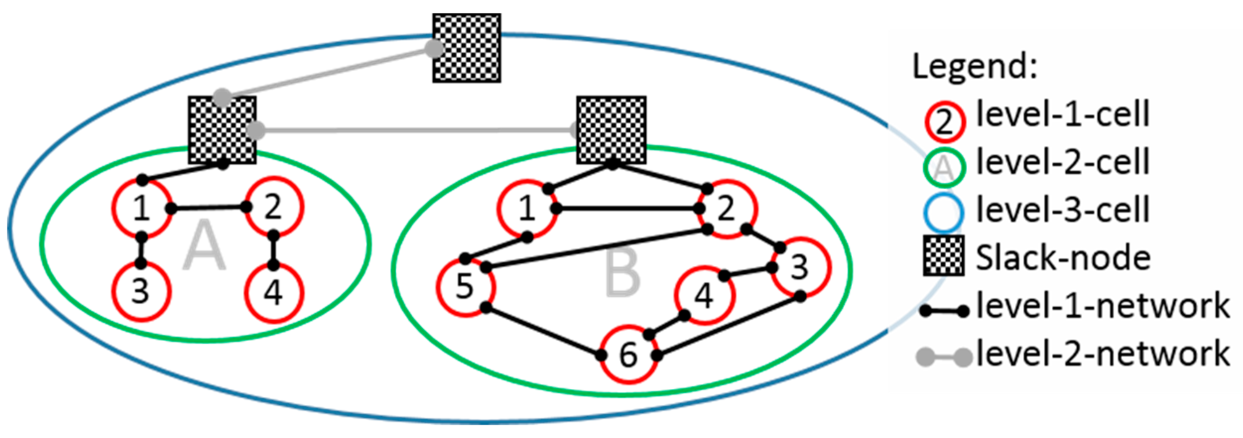
The cellular approach in HyFlow is implemented at three different cell levels. The lowest cell-level, a level-1 cell, contains residual loads, energy storage, hybrid elements and network connections between level-1 cells. Since HyFlow can adapt to various sizes of system boundaries via the cellular approach, a level-1 cell can be represented for instance by smaller units such as households or larger units like city districts or entire regions. The level-2 cell should be accordingly sized one aggregation level above and must consist of at least one level-1 cell. This is necessary because all data regarding energy demand or energy supply is specified exclusively in level-1 cells.

As seen in Figure 2, most level-2 cells will consist of several level-1 cells. It is imported to note, that no load flows within level-1 cells are considered. The network between level-1 cells, however, is the first target of the power flow calculation. The residual load of one specific level-2 cell is the result of balancing all corresponding level-1 cells, including possible losses within the level-1-network (dependent on load flow calculations). To transfer energy from superior cell level to a lower cell level or vice versa, a slack-node is used. Due to the chosen mathematical procedure (Newton–Raphson) only one slack-node can be used per cell to transfer energy from one cell level to another. However, each slack-node may have several network connections. Further properties of a level-2 cell, such as the current state of charge (SOC) and operational status of existing hybrid elements, are the sum of all assigned level-1 cells. A level-3 cell represents the highest cell level, and must contain all level-2 cells. It represents the overall system boundary. Analogous to the level-2 cell, the residual load of the level-3 cell is the result of the calculations in the level-2 domain. The remaining residual load in the level-3 cell has to be balanced from outside the system boundary, via the level-3 slack node. According to the presented goal of the cellular approach in Section 3, the target is to minimize the energy obtained from outside the system boundary and the maximum load flows over the level-3 slack node. Figure 2 displays an example of a possible scenario for the application of the cellular approach in HyFlow. It contains 10 level-1 cells, which are categorized in two level-2 cells. The level-2 cell A contains four, level-2 cell B six level-1 cells. The network connecting level-1- and level-2 cells as well as slack-nodes is also shown in Figure 2.

4.2. Modelling Framework Components

The following sections show how the most important system elements are characterized in HyFlow. The key components are the energy generation and demand, the energy storage units, and the hybrid elements necessary for the sector coupling and grid connections.

4.2.1. Energy Generation/Demand

Energy generation and demand in HyFlow is implemented by the use of residual loads for each energy carrier and level-1 cell. The residual load is defined as power demand minus power generation as shown in Equation (1). When considering all three implemented energy carriers, the usage of residual loads instead of separate data for production and demand allows the reduction from six necessary values to three values for each time-step.

$$P_{Res}\left[t\right]= P_{Load}\left[t\right]- P_{Gen}\left[t\right]$$

(1)

In case of a negative residual load, the cell is a net energy producer, a positive residual load represents a net demand for energy. Each level-1 cell has to be defined for each time step and energy carrier before using HyFlow. A possible source for residual loads is either measured data, load or generation profiles. Level-2- and level-3 cells are not specified with generation or demand data as the residual loads in higher cell levels are solely the result of the calculations in HyFlow.

4.2.2. Energy Storage

Energy storage in the HyFlow modelling framework is used to balance demand and production over time. For each level-1 cell and energy carrier one corresponding energy storage can be defined. As most energy storage units on a system level (batteries, pumped hydro, compressed air, flywheels, district heating storage tanks) are able to respond within seconds [38,39] to less than 10 min [40,41] to changes in demand, HyFlow does not consider ramp rates for energy storages. In case of a chosen smaller interval length of time steps compared to the technologies’ ramp rates, certain deviations in the results may occur. Results may deviate if the selected time step is smaller than the technology’s ramp rate. All characterization parameters are to be found in

Table 1. Generic energy storage characterization in HyFlow.

Parameter	Value [Unit]	Description
Storage capacity	positive [Wh]	Maximum energy storage capacity of the corresponding energy storage.
Maximum charge and discharge power	positive [W]	Maximum charge and discharge power of the corresponding energy storage.
Operation mode	0/1	This parameter defines if the energy storage operates in cell-serving- (parameter = 0) or system-serving-mode (parameter = 1). If the energy storage operates in cell-serving-mode it operates according to the residual load of the associated cell only. In the system-serving-mode the energy storage operates in response to the systems residual load, enabling third-parties to access the energy storage capacity.
Efficiency charge/discharge	0–1	This value represents the efficiency of the charging - and discharging process.
Self discharge	0–1 [1/h]	The time based efficiency considers self-discharge of energy storage within a time period of one hour.

.

The necessary parameters to define an energy storage unit in the HyFlow modelling framework are explained in the following table. This rather generic approach allows one to model a wide variety of energy storage units and other flexibility options like demand side management (DSM) in all energy carriers and enables the user to quickly change parameters in terms of technology improvements. Aging effects, such as reduced capacity of batteries over its life cycle, depth of discharge or other detailed effects like thermic stratification in thermal storage units are neglected in the model.

4.2.3. Hybrid Elements

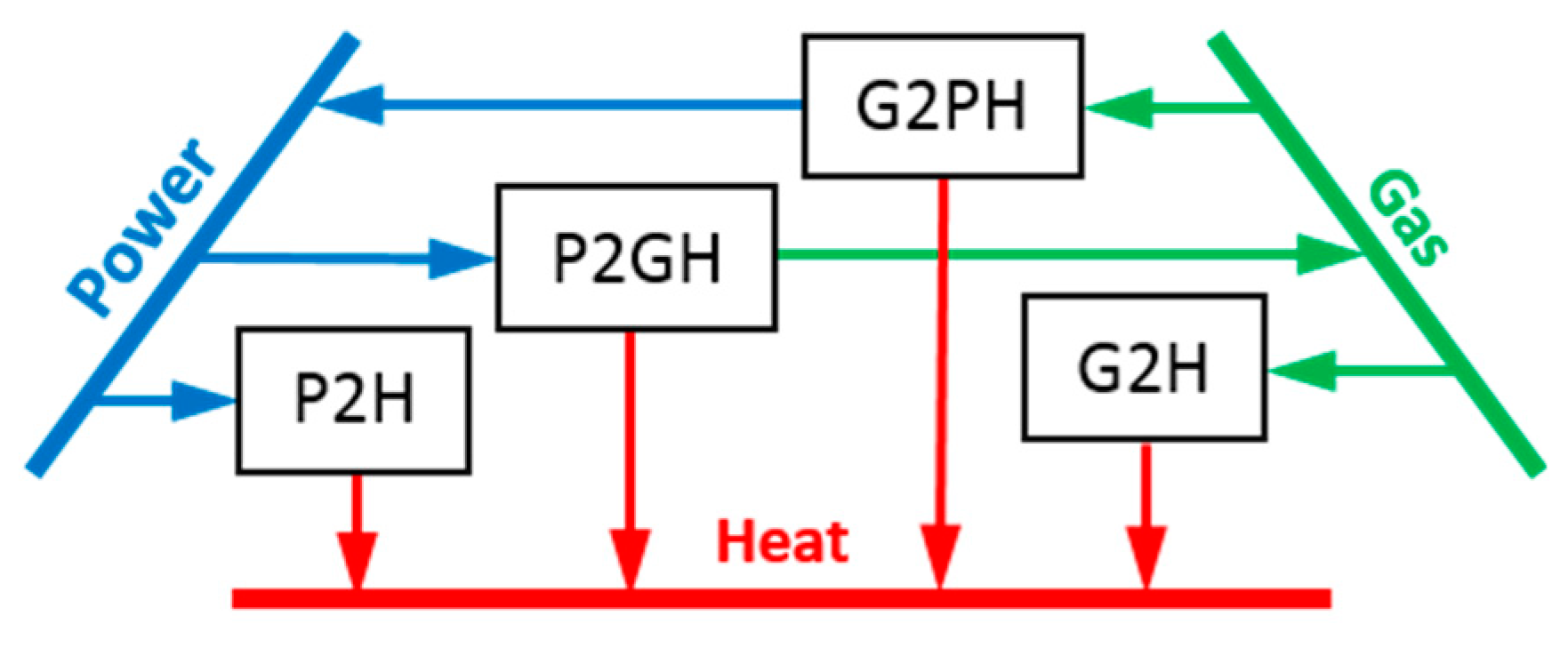
In order to enable the conversion from one energy carrier into another, hybrid elements are implemented in HyFlow. For each level-1 cell only one hybrid element can be defined. This limitation is necessary due to the possibility of a large number of very different deployment scenarios, if more than one hybrid element were included. Based on three separate energy carriers, up to six different hybrid technologies could theoretically be defined (P2H, P2G, G2P, G2H, H2P, H2G). However, today’s technological and economic environment focuses on four different kinds of hybrid element technologies as seen in Figure 3. The four implemented sector coupling possibilities are P2H (power to heat), P2GH (power to gas and heat), G2PH (gas to power and heat) and G2H (gas to heat). It is also possible to generate power from heat sources, but in the context of HyFlow the heat segment is seen on temperature levels of district heating grids at around 60–130 °C [42]. The efficiency of process technologies that generate power from heat at this temperature are very low (Organic Rankine Circle (ORC) process—well below 20% [43]) and economic feasibility is usually not possible.

P2H can represent any technology that converts electricity into power. On a household level this may be a heat pump or a heating rod, while high-voltage electrode boilers can be an example for a P2H plant at a utility level. P2G is a technology where hydrogen is produced via electrolysis and can be further processed via methanation to natural gas. If the infrastructure connection and the demand allow it, the resulting heat can also be utilized, which makes the technology to P2GH. If there is no option for waste heat utilization, the heat term remains 0. G2PH is the abbreviation of gas to power and heat. Examples of this technology are (micro) gas turbines, combined cycle gas turbines, fuel cells or ICE based combined heat and power units (CHP). Analogous to the P2GH technology, the heat term only applies if the occurring heat can be utilized. The last implemented hybrid element is G2H. This can be a gas boiler for heating purposes.

All four aforementioned hybrid elements and their implementation in hybrid grids must be further characterized. The necessary parameters to define a hybrid element in the HyFlow modelling framework are displayed in the following

Table 2. Characterization parameters for hybrid elements.

Parameter	Value [Unit]	Description
Maximum power	positive [W]	Defines the maximum power of a hybrid element. The maximum power is always related to the input factor.
Positive/Netative ramp rate	positive [1/h]	The positive/negative ramp rate defines the maximum increase/decrease of hybrid element power within a one-hour-period.
Electricity conversion efficiency	∊ ℝ [1]	The electricity conversion efficiency defines the percentage of maximum power to be converted into electricity. Following values for conversion efficiency power are possible: Conversion efficiency = 1: electricity is an input factor Conversion efficiency < 0: electricity is generated Conversion efficiency = 0: no electricity is generated
Heat/Gas conversion efficiency	∊ ℝ [1]	The heat/gas conversion efficiency defines the percentage of maximum power to be converted into heat/gas. The range of values for efficiency heat conversion is allowed to exceed the value of 1 are allowed for heat pumps.
Operation mode	0/1	This parameter defines if the hybrid element operates in response to a specific cells residual load (parameter = 0) or in response to the electrical residual load of the whole system (parameter = 1).

. In contrast to energy storage technologies, ramp rates are considered for large hybrid elements. This means that a threshold value for a nominal power of hybrid elements must be defined. All hybrid elements above that value consider the specified ramp rates, and the elements not exceeding the limit are neglecting any ramp rates.

4.2.4. Grids

In order to perform load flow calculations in all three energy carriers considered (as described in Section 4.3) the network interconnections between the level-1 cells and the level-2 cells must also be characterized. The grid is used to overcome the fact that energy is often produced at a different location to where it is required. Since the properties of the networks vary for the individual energy carriers the characterization differs among them. A similarity for all energy carriers is the way interconnections are characterized. This works through a linkage matrix. When there is a direct connection between cells, the linkage matrix L shows the value 1, if there is no direct connection, the according value is 0. In practice, linkage matrices are not limited to the values 0 and 1, but are used for important characterization values already. This means that for an electricity grid the matrix used contains the assigned length, reactance or resistance of the power line. This helps to compress necessary input data for the following load flow calculation into a single matrix.

4.3. Load Flow Calculations

As mentioned in Section 4.2, the power flow or load flow calculations (LFC) differ between energy carriers. However, it was important in the creation of HyFlow to make equivalent mathematical procedures in order to link the energy carriers and allow the calculations to work with acceptable computational times. The following sections describes the procedure of the load flow calculations for electricity, natural gas and district heating and point out the similarities among them.

4.3.1. Electricity Grid Load Flow

As described in Section 2, there are various possibilities to describe the power flow in electricity grids. Due to the stated reasons, the DC load flow calculation was selected as the model of choice for the tasks at hand. Since HyFlow is designed to work in use cases of a wide range of scales two different load flow calculation methods are included. The first (regular) DC load flow calculation method is a standard approach, as described in van Hertem et al. [44]. In order to simplify the power flow system the following assumptions are made:

• Reactive power flow is neglected
• All voltages correspond to the set nominal voltage
• Line resistances are negligible (X >> R)
• Voltage angle differences are small (sin (θ) $\approx$ θ)

The DC model with its corresponding equations is solved with the Newton–Raphson method. The simplified approach is presented in Equations (2) and (3). Equation (2) presents the active power transport between two nodes connected via a power line. Equation (3) is a direct consequence of the assumptions applied to Equation (2).

$$P_{Line}= \frac{\left|U_i\right|·\left|U_j\right|}{X_{Line}}·\sin \left(\theta \right)$$

(2)

$$P_{Line}= \frac{\theta }{X_{Line}}$$

(3)

The second electrical load flow calculations available in HyFlow is a modification of the standard DC load flow calculation. It neglects the active power transportation via phase angle and assumes a grid dominated by line resistances (R >> X). The active power transportation is, therefore, caused by a change in node voltages and the power losses are no longer neglected. This approach corresponds to a grid, which is operated in DC. Equation (4) shows the calculation of the complex apparent power (S_i), which can be calculated by multiplying the node voltage (U_i) by the conjugated complex node current (I_i*). It is both valid for AC and DC applications. Under the given constraints, the imaginary parts of the node current, node voltage and the nodal admittance are neglected, which is demonstrated in Equations (5) and (6). This means that no reactive power is considered and the apparent power equals the active power. The computational method is a Newton–Raphson method again, with the difference that the parameter to be varied is the node voltage instead of the phase angle of the voltages.

$${\underset{\_}{S}}_i={\underset{\_}{U}}_i\ast {\underset{\_}{I}}_i^{\ast }={\underset{\_}{U}}_i\ast {\left({\displaystyle \sum }_{j=1}^n{\underset{\_}{Y}}_{ij}\ast {\underset{\_}{U}}_j\right)}^{\ast }$$

(4)

$$Im\left({\underset{\_}{I}}_i,{\underset{\_}{U}}_i,{\underset{\_}{Y}}_{ij}\right)=0$$

(5)

$$P_{ij}=U_i\left(U_j-U_i\right)\ast Y_{ij}$$

(6)

In HyFlow, the first DC load flow methodology and the corresponding assumptions are applied to high-voltage grids, the second methodology is applied to resistance-dominated low-voltage grids. The final decision, which load flow calculation is the appropriate method must be made by the user.

4.3.2. Pipeline Network Load Flow

The load flow calculations in pipeline networks have one significant difference to electrical grids. While the behavior of electrical grids can be described with Ohm’s linear law, the dependencies of mass flows in pipelines show a quadratic correlation described by Darcy’s law. There are, however, also similarities to the electrical grid, as shown in the following Equations (7)–(9). The pressure difference is equivalent to the voltage drop and the volume flow represents the current in electrical grids.

$$\Delta p\stackrel{\wedge}{=}\Delta U$$

(7)

$$\dot{V\stackrel{\wedge}{=}I}$$

(8)

$$\Delta U=R·I \stackrel{\wedge}{=} \Delta p_{loss}= \frac{\lambda ·l·\rho ·8}{d^5·{\pi }^2}·{\dot{V}}^2$$

(9)

The quadratic dependency between the pressure loss and the volume flow can clearly be seen. Additionally, it should be noted that additional input variables are necessary to characterize the grid. These values are the friction factor, the density of the medium and the inner diameter of the pipeline. In order to linearize the equation and solve it in a way that is analogous to the electrical grid, the following procedure according to the Equations (10) and (11) is performed:

$$\Delta p_{loss}= R^{\ast }·\dot{V}$$

(10)

$$R^{\ast }=\frac{\lambda ·l·\rho ·8}{d^5·{\pi }^2}·\dot{V}$$

(11)

The quadratic volume flow is separated and a term $\dot{V}$ is assigned to the analogous resistance value of the electrical system $R^{\ast }$. This allows to transfer the calculation procedure of the electrical grid to the natural gas grid. The Darcy equation as an iterative procedure can be formulated as follows:

$$\Delta p_{loss \left(t\right)}= \frac{{\lambda }_{ij \left[t-1\right]}·l·\rho ·8}{d^5·{\pi }^2}·{\dot{V}}_{\left[t-1\right]}·{\dot{V}}_{\left[t\right]}$$

(12)

Subsequently the nominal node pressure levels and the edge pressure losses in the individual pipeline sections can be determined. Analogous to the electrical system, the volume flows can be calculated from the pressure differences between connected nodes. Since the solution of the quadratic equation does not allow the determination of the sign of the volume flow and the according flow direction the sign function is used to solve this problem as seen in Equation (13). The sign function returns −1, if $\Delta p_{loss, ij \left[t\right]}$ equals any negative number and +1, if the pressure difference is positive. This ensures the correct correct direction of flow and numeric value of the flow rate. The friction factor ${\lambda }_{ij}$ is a function of the Reynolds number $R{e}_{ij }$, which is again a function of the flow rate ${\dot{V}}_{ij}$. Therefore, the determination of these values follows an iterative process described in Rüdiger [45]. The conversion from the flow rate ${\dot{V}}_{ij}$ to the necessary transported power flows can be described by Equations (14) and (15).

$${\dot{V}}_{ij \left[t\right]}=sign \left(\Delta p_{loss, ij \left[t\right]}\right)·\sqrt{\frac{d^5·{\pi }^2}{{\lambda }_{ij \left[t-1\right]}·l·\rho ·8}·\left|\Delta p_{loss, ij \left[t\right]}\right|}$$

(13)

$${\dot{V}}_{Gas,ij}=\frac{P_{Gas,ij}}{{\rho }_{Gas}·h_U}$$

(14)

$${\dot{V}}_{Heat,ij}=\frac{P_{Heat,ij}}{{\rho }_{Water}·c_p·\left(T_{in}-T_{out}\right)}$$

(15)

4.4. Program Work Flow

The following three sections describe the workflow of HyFlow. It shows which input parameters need to be specified by the user and how the calculation process is structured and performed by the program. The third section shows the wide variety of results that can be obtained by running HyFlow.

4.4.1. Input Parameters

Input parameters in HyFlow have to be defined in separate ways depending on the parameter. Parameters like the maximum number of level-1 cells, the slack node voltage and the pressure in level-1- and level-2-grids, tolerances and limits for the activation of system serving hybrid elements have to be defined in a MATLAB^® interface. Further necessary data such as residual loads of cells, properties of storages and hybrid elements and network parameters for level-1 and level-2 grids have to be stored in EXCEL^® files. After the EXCEL^® files are read by MATLAB^®, a function checks all input data. If a deviation is detected, MATLAB^® displays an error message, and shows the user which data is not supplied in the correct form.

Table 3. Prepared input data files in excel.

Parameter	Value [Unit]	Description
level-1 cell residual load	[W]	Power, heat and gas residual load for each level-1 cell
power level 1 network_	[Ω] [θ] [m]	Resistance, phase angle, length between two nodes.
heat level 1 network diameter	[m]	Diameter of pipe between two nodes.
heat level 1 network length	[m]	Length of pipe between two nodes.
heat level 1 network roughness	---	Roughness of pipe between two nodes.
heat level 1 network thermal conductivity	[W/(m*K)]	Thermal conductivity of pipe between two nodes.
gas level 1 network diameter	[m]	Diameter of pipe between two nodes.
gas level 1 network length	[m]	Length of pipe between two nodes.
gas level 1 network roughness	---	Roughness of pipe between two nodes.

provides an overview about necessary input data. Network parameters shown in Table 3 must be available for level-1 and level-2 cells.

4.4.2. Calculations and Program Sequence

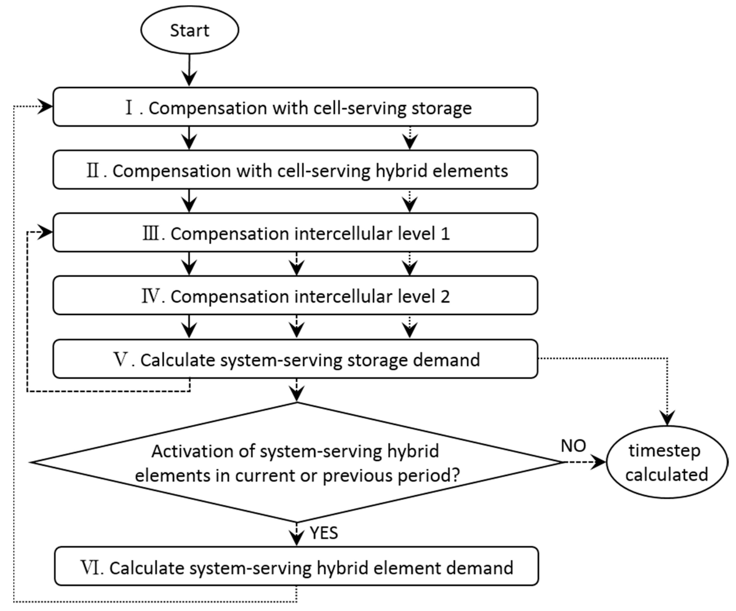
The presented program workflow is designed to follow the introduced cellular approach to balance supply and demand at the lowest possible cell-level. This approach is present at every system level of HyFlow. If a local energy source of any carrier is available, it will always be prioritized over obtaining energy from the superior grid level. However an important condition is that all energy demand needs to be met at any time. If this condition is violated for any reason, an error occurs. After the user has specified the system and has provided the necessary residual loads, network connections and properties, storage units, and hybrid elements, the actual calculation process begins according to Figure 4.

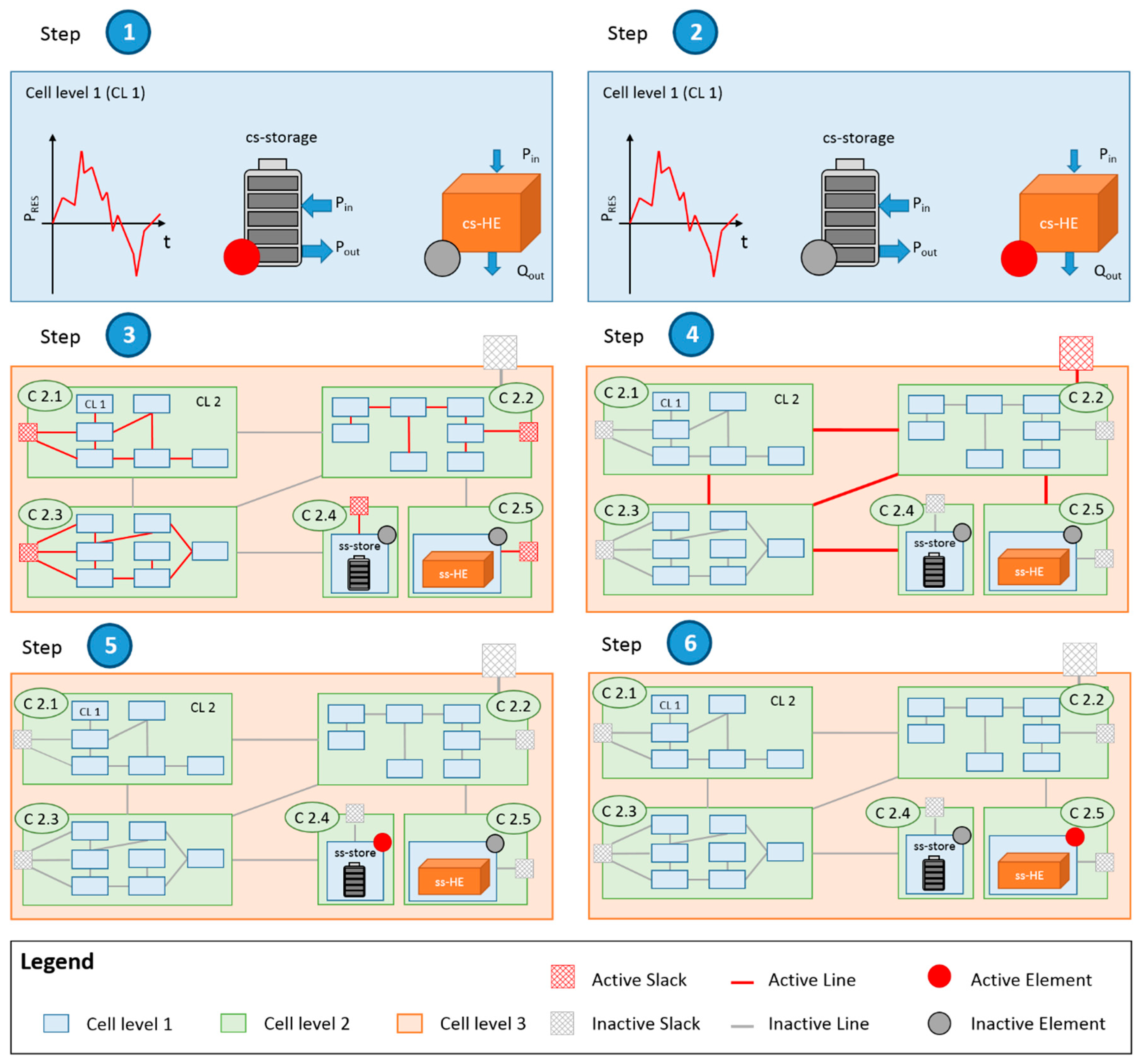
Step 1—Compensation with cell-serving storage

In the first step, any available storage in a level-1 cell is used in order to minimize the residual load of the corresponding level-1 cell. The algorithm that is used, is the “greedy” algorithm: As soon as the residual load of a cell is negative and storage capacity is available, the excess energy generation is stored in the available storage unit. When the residual load turns positive again, energy is immediately prioritized from the storage over the grid. The difference between a cell-serving element and a system-serving element is the associated control strategy. While cell-serving elements minimize solely the residual load of the containing cell (greedy algorithm), the system-serving elements switch on and off based on the residual load of the overall system boundaries (level-3), by using the greedy algorithm as well. A graphic illustration of all process steps is shown in Figure 5. All elements marked in red are active in the corresponding process step.

Step 2—Compensation with cell-serving hybrid elements

The usage of cell-serving hybrid elements within a level-1 cell, is the next priority. This means that unbalanced residual loads paired with a full/empty storage unit of the same energy carrier lead to the use of cell-serving hybrid elements. For example, a negative residual load in the electricity network combined with a full electricity storage can lead to the usage of a heat pump, if there is either a heat demand in the cell or a heat storage that is not fully charged. In general, three control strategies are implemented in HyFlow for cell-serving P2H, G2H and G2PH hybrid elements. The control strategy of P2H as well as G2PH hybrid elements depends on various factors such as power and heat residual load and storage level of all energy carriers involved. A G2H hybrid element balances heat demand and, if possible, charges the heat storage. It is also possible that a hybrid element is not used as a flexibility option, but as a conventional energy supply source. In the example of a G2H element (e.g., gas boiler) and no connection to the heating grid, the heat demand is supplied over the gas grid.

The mathematical description of an exemplary P2H device is described below: If the residual load $P_{Res\left[t\right]}$ is negative, while the heat demand $Q_{Res\left[t\right]}$ is positive and the absolute value of the residual load $\left|P_{Res\left[t\right]}\right|$ multiplied by the conversion efficiency from power to heat ${\eta }_{PQ}$ is the same or greater than the actual heat demand $Q_{Res\left[t\right]}$, the total heat demand can be met by the residual load of the electricity $P_{Res\left[t\right]}$. This means that the new heat demand in this time-step $Q_{Res,new\left[t\right]}$ is 0, while the residual load $P_{Res,2\left[t\right]}$ becomes less negative by adding the converted power to the original $P_{Res\left[t\right]}$. Afterwards, the new variable is overwritten for reasons of the further calculation process.

$$\{P_{Res,2\left[t\right]} \wedge Q_{Res,new\left[t\right] }|\left(P_{Res\left[t\right]}\langle 0 \wedge Q_{Res\left[t\right]}\rangle 0\right)\wedge \left(\left|P_{Res\left[t\right]}\right|·{\eta }_{PQ})\ge Q_{Res\left[t\right]}\right)\}$$

$$Q_{Res,new\left[t\right]}=0$$

(16)

$$P_{Res,2\left[t\right]}=P_{Res\left[t\right]}+\frac{Q_{Res\left[t\right]}}{{\eta }_{PQ}}$$

(17)

$$P_{Res,2\left[t\right]}=P_{Res\left[t\right]}$$

(18)

The Equations (19)–(21) work under the same condition than before with the exception that the absolute value of the residual load $\left|P_{Res\left[t\right]}\right|$ multiplied by the conversion efficiency from power to heat ${\eta }_{PQ}$ is now smaller than the heat demand $Q_{Res\left[t\right]}$. This implies that the remaining residual load of power $P_{Res,2\left[t\right]}$ amounts 0 at the end of the process and the new remaining heat demand $Q_{Res,new\left[t\right]}$ is reduced by the converted power multiplied with conversion efficiency ${\eta }_{PQ}$.

$$\{P_{Res,2\left[t\right]} \wedge Q_{Res,new\left[t\right] }| \left(P_{Res\left[t\right]}\langle 0 \wedge Q_{Res\left[t\right]}\rangle 0\right)\wedge \left(\left|P_{Res\left[t\right]}\right|·{\eta }_{PQ})<Q_{Res\left[t\right]}\right)\}$$

$$P_{Res,2\left[t\right]}=0$$

(19)

$$Q_{Res,new\left[t\right]}=Q_{Res\left[t\right]}-\left(\left|P_{Res\left[t\right]}\right|·{\eta }_{PQ}\right)$$

(20)

$$P_{Res,2\left[t\right]}=P_{Res\left[t\right]}$$

(21)

The residual power $P_{Res\left[t\right]}$ can also be converted to heat in a cell-serving P2H element if no heat demand occurs or has been met by the hybrid P2H element before already, by the usage of a heat storage unit. If the heat storage unit is not full at the time step of the calculation and surplus power is available it can be stored as heat. There are two options again: Equations (23) and (24) describe the situation, where the energy of the residual power $P_{Res\left[t\right]}$ times the conversion factor ${\eta }_{PQ}$ is greater than the remaining storage capacity.

$$\begin{array}{c}\{P_{Res,new\left[t\right]}\wedge SO{C}_{Q,new\left[t\right]} |\left(P_{Res\left[t\right]}<0 \wedge \left(Q_{Res\left[t\right]}<0 \vee Q_{Res,new\left[t\right]}=0\right)\right)\wedge (SO{C}_{Q\left[t\right]}\\ <SO{C}_{Q,max}) \wedge (\frac{\left|P_{Res\left[t\right]}\right|}{t_{int}}·{\eta }_{PQ}>\left(SO{C}_{Q,max}-SO{C}_{Q\left[t\right]}\right)\}\end{array}$$

$$t_{int}=\frac{timesteps}{hour}$$

(22)

$$P_{Res,new\left[t\right] }=P_{Res\left[t\right] }+ \frac{\left(SO{C}_{Q,max}-SO{C}_{Q\left[t\right]}\right)·t_{int}}{{\eta }_{PQ}}$$

(23)

$$SO{C}_{Q,new\left[t\right]}=SO{C}_{Q,max}$$

(24)

The second option is described by Equations (25) and (26). The energy of the residual load of electricity $P_{Res\left[t\right]}$ is smaller than the available heat storage capacity. This results in a new residual load $P_{Res,new\left[t\right]}$ of 0 and a new heat storage content $SO{C}_{Q,new\left[t\right]}$ described by Equation (25). Another option in the P2H elements in HyFlow is the usage of stored electricity for the heat demand as well. This option and other hybrid elements such as G2PH or G2H work analogous to the described example below.

$$\begin{array}{c}\{P_{Res,new\left[t\right] }\wedge SO{C}_{Q,new\left[t\right]} |\left(P_{Res\left[t\right]}<0 \wedge (Q_{Res\left[t\right]}<0 \vee Q_{Res,new\left[t\right]}=0)\right)\wedge (SO{C}_{Q\left[t\right]}\\ <SO{C}_{Q,max}) \wedge (\frac{\left|P_{Res\left[t\right]}\right|}{t_{int}}·{\eta }_{PQ}<\left(SO{C}_{Q,max}-SO{C}_{Q\left[t\right]}\right)\}\end{array}$$

$$SO{C}_{Q,new\left[t\right]}=SO{C}_{Q\left[t\right]}+\left(\left|P_{Res\left[t\right] }\right|·t_{int}·{\eta }_{PQ}\right)$$

(25)

$$P_{Res,new\left[t\right] }=0$$

(26)

Step 3—Compensation intercellular level 1

The aim of this step is to balance the residual load of each level-2 cell by shifting energy between level-1 cells in the assigned level-2 cell. All level-1 cells within the level-2 cell are considered and the load flow calculations described are performed for all energy carriers. Additionally storages of other cells in the same level can be accessed by other cells, if the storage units are defined as system-serving. Cell-serving storages can only be accessed by the containing cell itself. The residual load of the total level-2 cell contains network losses within the grid between level-1 cells. The detailed description of this step and the performed load flow calculations, including the necessary equations can be found in Section 4.3 load flow calculations.

Step 4—Compensation intercellular level 2

When the balancing within the level-2 cells is completed, the resulting residual loads (including calculated losses of transport lines, losses of storages and hybrid elements) are transferred to the second level. A new load flow calculation analogous to the level-1 cells is performed. Since the characterization of system-serving storages is done on the level-1 cell, the storage terms in this level are considered “virtual” and are calculated as the sum of properties of all system serving storages of level-1 cells in the corresponding level-2 cell. The calculation process and the “greedy” algorithm is used in the exact same way as described in step 1. The residual load of the level-3 cell also contains network losses within the grid between level-2 cells. If energy storage is used in this step, any changes in storage capacities have to be retransferred to level-1 cells, and therefore step 5 is necessary.

Step 5—Calculate system-serving storage demand

Since only “virtual storages” are used in step 4, any change in storage capacity must be retransferred in level-1 cells. Therefore, the change of storage capacity has to be carried out in all level-1 cells. If more than one level-1 cell has free capacities in energy storage, the new load flow is divided among them in an iterative process that aims to fill storage units to the same amount. This process step, however, also affects the residual load of selected cells and the load flows within the level-2 cell. To cope with these changes, functions similar to step 3 and step 4 have to be executed again, to update both residual loads and grid losses.

Step 6—Calculate system-serving hybrid element demand

System serving hybrid elements are only activated or deactivated if there is a residual load in the level-3 cell. In case of a power shortage, available G2PH hybrid elements are either ramped up to balance demand or ramped up to maximum power generation if power demand exceeds maximum power. Furthermore, all P2GH hybrid elements are ramped down to the lowest possible power consumption. In case of an excess of power, opposite measures are taken. All G2PH hybrid elements are ramped down to their minimum output, whereas P2GH and P2H hybrid elements are activated. If the electric residual load is close to 0 (within a specified tolerance), all system-serving G2PH and P2GH hybrid elements are ramped down to their lowest possible performance. If any system-serving hybrid elements were running in the current or prior time-step, steps one to five must be repeated, because they affect all other load flows significantly.

After all time steps are calculated a plausibility check is performed by calculating a separate energy balance for each time-step. If a defined tolerance is exceeded, HyFlow displays a warning message.

4.4.3. Results and Visualization

HyFlow gives the user the possibility of a wide range of results and visualizations. Depending on the focus of the user, various priorities can be defined. It is possible to model the status quo of a given region, with all the load flows one wants to consider. The focus can be on the voltage level of a critical power line within a distribution network, on the degree of self-sufficiency of a city quarter or district or on the effects of flexibility options like storage or sector-coupling technologies on the energy system. All pressure levels, voltages, load flows, power losses etc. can be displayed, analyzed and evaluated by the user. A main result is also the residual load of the total system (level-3 cell) and the maximum power in the slack-node over the analyzed time frame to design infrastructure properties of network connections of hybrid elements. Another aspect is the chosen control strategy which allows us to answer the question of whether a system-serving environment for energy storage units and hybrid elements can have positive effects on the overall system. These results are used to plot charts, to provide an overview about stored, consumed and produced power for each energy carrier and comment on how residual loads may be minimized by the use of storages and hybrid elements.

5. Results

Within this paper, two case studies are investigated. All case studies are based on a mixture of measured and modeled data, which is adapted and supplemented to demonstrate different application cases of the modelling framework. The main purpose of the use cases presented is to give an overview on expected results and deepen the understanding of the modelling frameworks functionality. Case study 1 considers an urban energy system, which is used to show HyFlow’s ability to calculate load flows of all three energy carriers in meshed networks. Case study 2 describes the interaction of the modelled city from case study 1 with its surrounding districts. This case study is implemented in HyFlow in order to point out the ability to simulate scenarios with two different voltage levels (or pressure levels for natural gas networks) and to show the influence of large P2G plants. All simulations are conducted over a 1-year time horizon, using 15 min time-steps.

To show the effect of fluctuating generation, temporarily high consumption due to charging processes for electric vehicles (EV), as well as the effect of energy storage and sector coupling, three scenario levels are selected for both case studies. After solving the reference scenario, which shows the status quo power flow situation without PV and EV penetration, the mentioned technologies (PV and EV) are implemented into the high-stress scenario with high penetration rates. Finally by taking storage technologies and hybrid elements into account, two improvement scenarios are conducted in order to show the effects of the chosen flexibility options on the power flow situation.

The evaluation indicators used for all case studies and scenarios and the according equations are listed below. The KPIs for electricity are the maximum value of power for imports and exports over the whole year $P_{el,max,year}$ the average of the daily maxima for electricity power $P_{el,Ø max,day}$ and the overall imported and exported electric energy, natural gas and district heating $E_{el}$, $E_{gas}$ and $E_{heat}$.

The amount of energy imported into and exported out of the system as shown in the results are calculated by using Equation (27), with $P\left(t\right)$ being the actual power flow for the corresponding time interval.

$$E={\displaystyle \sum }_{t=1}^n\frac{P\left(t\right)}{t_{int}}$$

(27)

• $P_{imp}\left(t\right)$ corresponds to $P\left(t\right)$, but all negative values are set to zero
• $P_{exp}\left(t\right)$ corresponds to $P\left(t\right)$, but all positive values are set to zero
• $n$ is the total number of time-steps
• $t_{int}$ is the amount of time-steps per hour, e.g., for the calculation of 15-min values $t_{int}=4$.

It has to be stated that the described parameters are only KPIs for the overall system configuration. HyFlow additionally supplies the user with time-resolved data of all voltages, pressures, load flows, losses etc. for every single network connection within the model. Additionally the usage profile of every single storage unit or hybrid element can be selected and displayed. Since these detailed results would go beyond the scope of this work, the focus is on the energy import/export and power transmission within the overall system level.

5.1. Case Study 2: Medium-Sized City

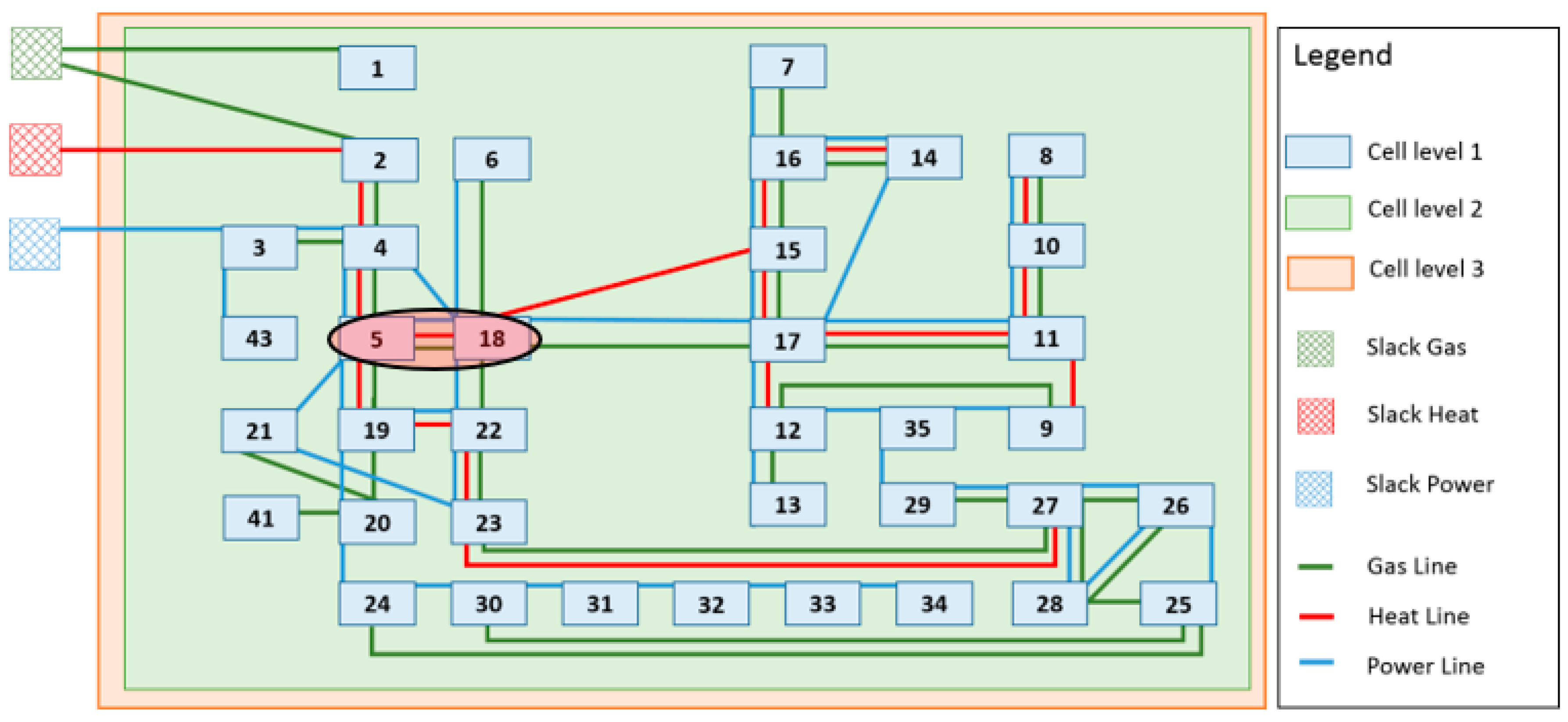
Case study 2 represents a medium-sized city in Austria, with around 30,000 inhabitants. The assumed city is divided into 44 cells within this work, based on its topology. All cells that contain grid-bound energy supply (el, heat, gas) can be seen in Figure 6. It shows an electrical medium voltage grid (blue), a district heating grid (red), and a natural gas grid (green). Some cells are connected to all three grids, while others are only connected to certain energy carriers. The investigated medium-voltage grid operates at a nominal voltage of 5.25 kV, the heat network operates at 17.5 bar and the gas distribution network at 4.0 bar.

A hydroelectric power plant (p.p.) (10 MW) and a biomass p.p. (3.6 MW) is available in all scenarios. The high-stress scenario includes PV generation of 43.5 GWh distributed over the cells, based on 50% of the evaluated solar roof potentials. Furthermore, a total number of 1600 EV (11 kW—max. charging power) is added, derived from the building count of the city. This follows the assumption that 25% of all single family homes own an EV and multi-family homes and apartment buildings are assigned one EV as well. In the improvement scenarios buildings are equipped with additional Li-ion batteries, heat storage units and heat pumps. The summarized chosen input parameters of case study 2 are shown in

Table 4. Configuration levels for case study 2.

Parameter	Reference Scenario	High-Stress Scenario	Improvement Scenario 1	Improvement Scenario 2
demand	standard	incl. 1600 EV	incl. 1600 EV (17.6 MW)	incl. 1600 EV (17.6 MW)
generation	1 hydro p.p. 1 biomass p.p	1 hydro p.p. 1 biomass p.p. PV potential	1 hydro p.p. 1 biomass p.p. PV potential	1 hydro p.p. 1 biomass p.p. PV potential
el. storages th. storages	-	-	el: 11.5 MWh—7.7 MW	el: 115 MWh—77 MW th: 128 MWh—14.4 MW
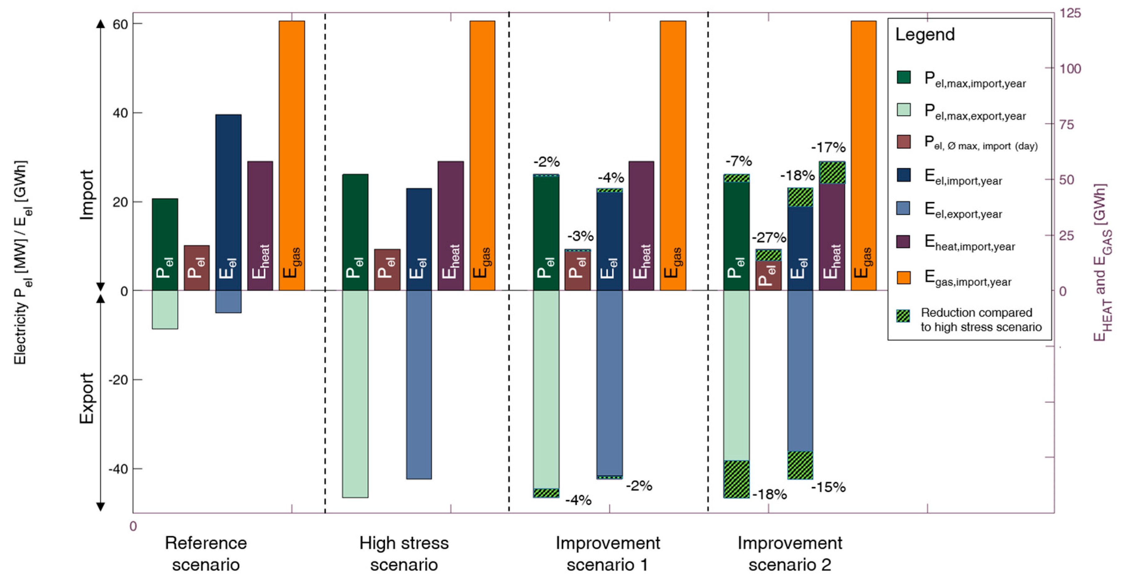
hybrid elements	-	-		Heat pumps: 15.8 MWth

. The results of case study 2 are shown in Figure 7. The annual maximum power import amounts to 20.7 MW and 39.5 GWh of electricity need to be imported, while the exported electricity sums up to 5.0 GWh with an annual maximum power export of 8.6 MW. The average daily maximum of power imports is 10.2 MW. The imported heat remains unchanged in the first three scenarios at 58.0 GWh and the gas imports are constant throughout the entire case study 2 at 121.3 GWh. Due to the significantly higher values compared to the electricity sector, the district heating and the natural gas values are depicted on the secondary vertical axis on the right of Figure 7. The biggest change in the results obtained can be seen between the reference scenario and the high-stress scenario. By adding the EVs and the PV potential, the positive and negative peaks of electrical power and the energy exports are increased. The annual maximum power import is increased by 5.4 MW and the maximum export power changes from 8.6 MW to 46.6 MW. It is interesting to see that regardless of the occurring higher annual peaks of imported power the average daily power maximum is slightly reduced from 10.2 MW to 9.3 MW. This is due to the fact that the maxima of electricity imports that arise are usually monitored around noon, where the PV power production peaks as well and reduces the necessary power of electricity imports. The high-stress scenario can be described by a lower electric energy import (23.0 instead of 39.5 GWh), a much higher electric energy export (42.3 GWh instead of 5.0 GWh) and a higher volatility of the occurring residual loads. The main outcome of improvement scenario 1 is, that the distribution of Li-ion batteries alone only marginally affects the peak powers and the electricity imports/exports. Even in improvement scenario 2 with a very high number of installed Li-ion batteries, heat pumps and heat storage units, the peak powers in electricity and the imported/exported energy can only be reduced partially. The district heating imports, however, decrease by 17%, because this heating demand is provided by the installed heat pumps. The gas imports stay constant in all scenarios, because no P2G technology is implemented in this use case.

5.2. Case Study 2: Region

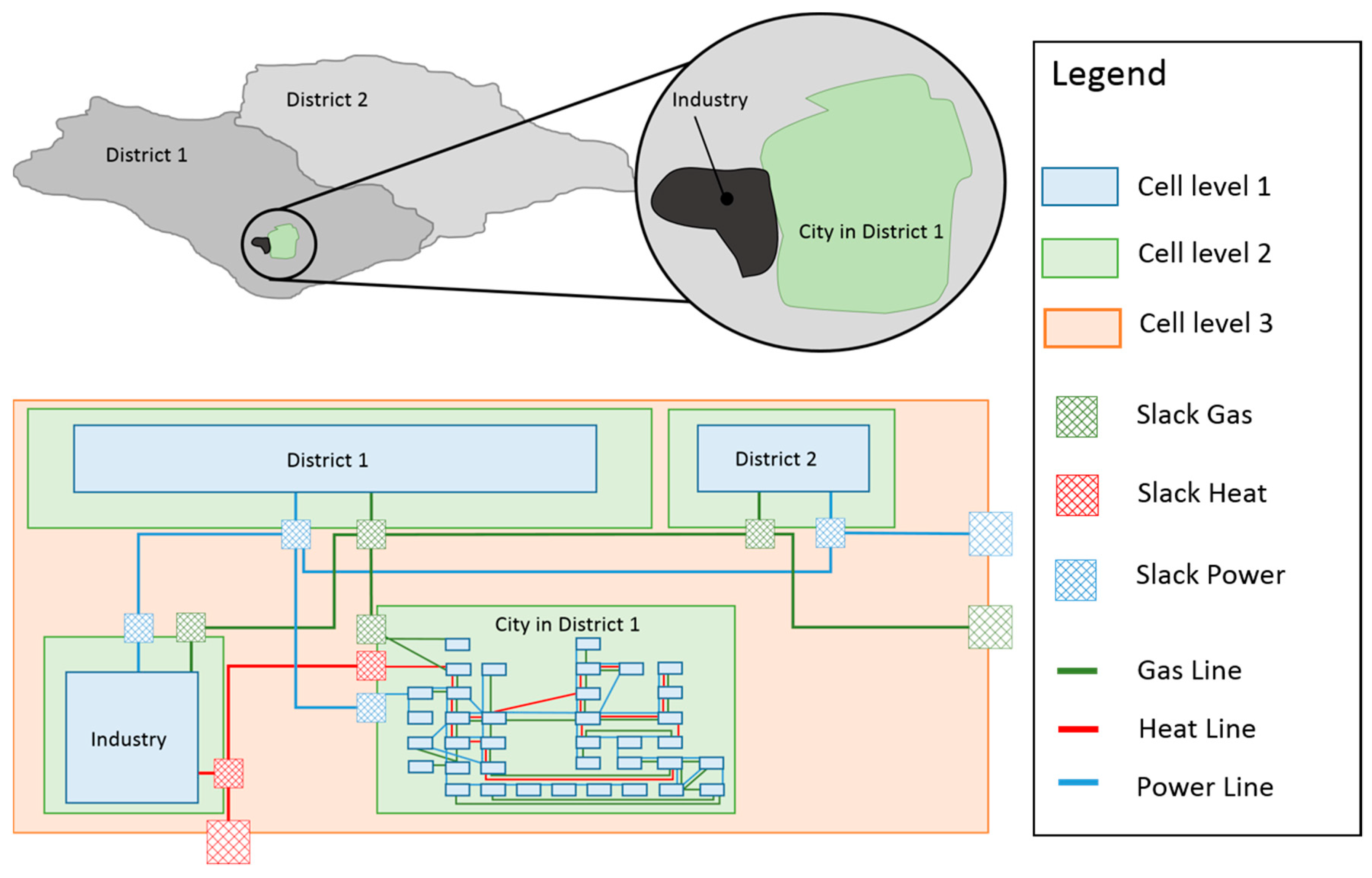
The third case study shows the interaction of the shown city from case study 1 with its surrounding region. This should demonstrate the modelling frameworks’ ability to perform calculations of different voltage—and pressure levels. To fulfill this task, the city from case study 1 (including all containing cells) is put next to a fictional industrial park in district 1. Together with a second district 2 they form the investigated system boundaries. Apart from the unchanged city cell from case study 1, all other level-2 cells contain only one level-1 cell. This means that all consumers, generation and storages in district 1 and 2 are not provided with the same detailed resolution as in the city cell. This structured view enables us to analyze the changed load flows of the city, with the embedding in its surroundings. However, it does not supply any information about the load flows within the mentioned districts themselves, since these districts were not equipped with the same detailed resolution as the city. The network connections of all energy carriers are illustrated in Figure 8. The grid parameters between level-1 cells remain unchanged compared to case study 1. However, the network connections of the electricity grid between level-2 cells have a nominal voltage of 110 kV at the slack node and the nominal pressure for the natural gas grid is assumed to be 60 bar.

The high-stress scenario includes an assumed PV potential of 87 GWh and 745 GWh in the other three level-2 cells based on the calculated solar rooftop potentials. By referring to the districts’ population in relation to the people living in the city of use case 1, the number of EV for each level-2 cell is calculated (7900 in total). The improvement scenarios include Li-ion-batteries, heat storage units and heat pumps. Additionally one P2G-plant (Pel = 500 MWel, η = 0.65) is placed in district 1. It operates as a system-serving hybrid element based on the electrical load flow and the gas demand of the overall system. The summarized input parameters of case study 2 are shown in

Table 5. Configuration levels for case study 2.

Parameter	Reference Scenario	High-Stress Scenario	Improvement Scenario 1	Improvement Scenario 2
demand	standard	incl. 7900 EV	incl. 7900 EV	incl. 7900 EV
generation	1 hydro p.p. 1 biomass p.p	1 hydro p.p. 1 biomass p.p. PV potential	1 hydro p.p. 1 biomass p.p. PV potential	1 hydro p.p. 1 biomass p.p. PV potential
storages	-	-	el: 57 MWh—38 MW	el: 57 MWh—38 MW th: 128 MWh—14.4 MW
hybrid elements	-	-		Heat pumps: 15.8 MWth
				P2G: 500 MWel—η = 0.65

.

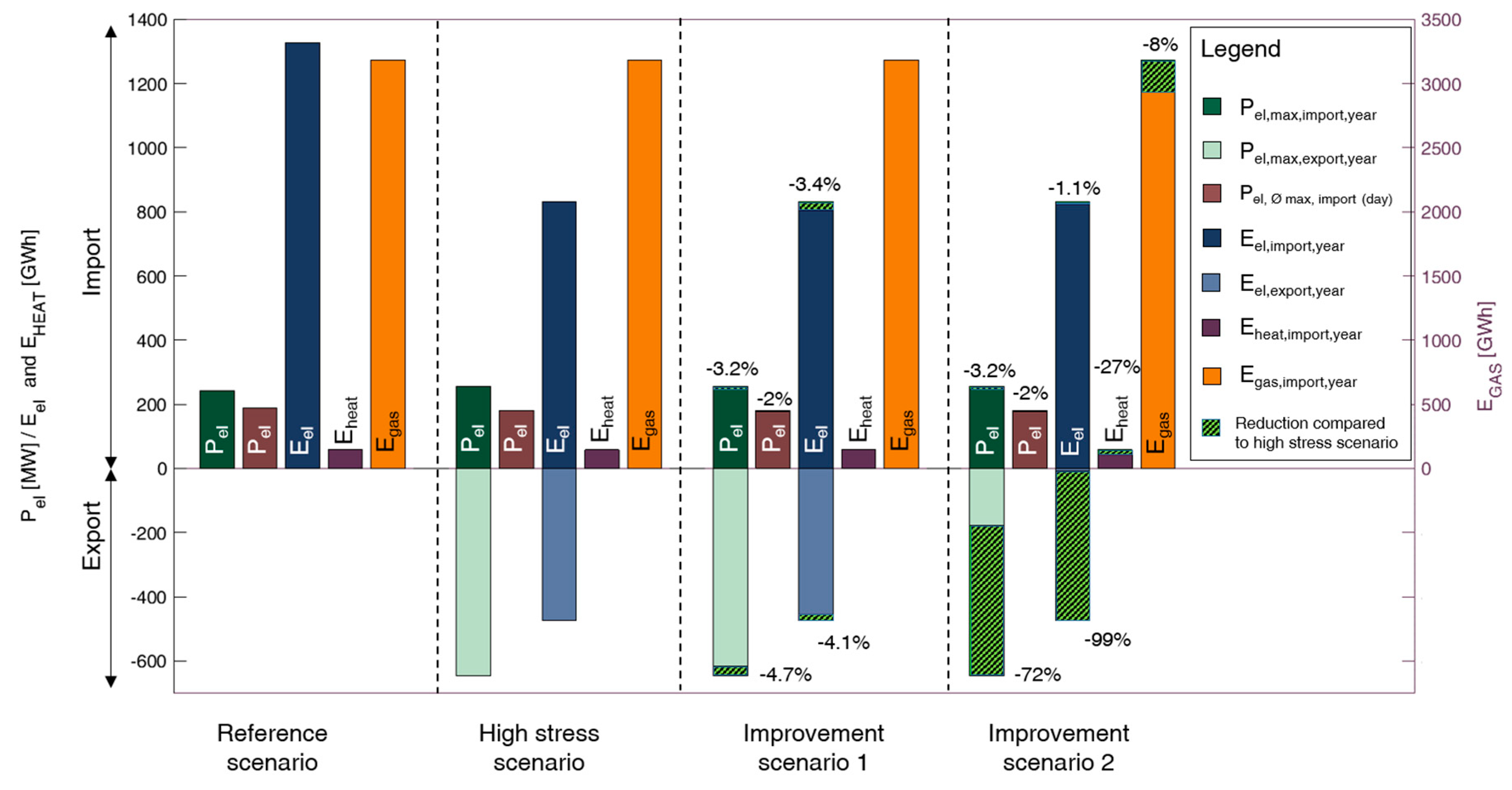
Figure 9 shows the results of all conducted scenarios of use case 2. The results of the reference scenario show the net energy demand of all energy carriers and power peaks of electricity of the analyzed area. By adding the described PV potential the electricity imports decline from 1326 GWh to 833 GWh. At the same time the maximum annual power peaks for imports are raised from 243 MW to 256 MW, and the export power peaks are increased from 0 to 646 MW. In improvement scenario 1 with added Li-ion batteries the maximum power and electricity imports/exports are slightly reduced.

A very big change, however, can be observed in improvement scenario 2. The large fictional P2G plant is capable of reducing almost the entire exported electric energy, by means of converting it to natural gas. The remaining exported power peaks of 248 MW are still high, but account for only just over 1% of the exported electricity, because these powers only occur on rare occasions. Examples for these occasions are higher surplus electricity than the maximum power of the P2G plant or unconvertible power peaks due to the implemented P2G ramp rate restrictions. The implementation of the sector coupling technologies are able to reduce the large natural gas imports by 8% (P2G) and the district heating demand by 27% (P2H).

Another way to visualize the time-resolved energy imports/exports over the whole year, as well as the calculated power maxima/minima are load duration curves, shown in Figure 10. This shows the sorted power exchange with the superior grid for all three energy carriers considered. One can see, that the electrical power duration curve greatly varies in the four scenarios. In particular, the difference between the reference scenario and the high-stress scenario is striking. Around 3000 h with negative residual loads and power exports caused by the added fluctuating generation is clearly visible. The improvement scenario 1 with added storage can add little to reduce exports, but the P2G plant in improvement scenario 2 is able to reduce almost all electrical power exports. This exact phenomena can also be observed in the visualization of P_Gas in Figure 10. At times where electrical exports are reduced by the P2G plant, the external demand of gas supply is greatly reduced. The P2G plant is not able to reduce load peaks in either the electrical or the gas imports. The visualization of the high-stress and the improvement scenario was waived due to the overlap with the reference scenario in P_th and P_Gas. In the district heating grid, the improvement scenario 2 with added heat pumps and distributed thermal storage units succeeded in reducing the imports throughout the year. The necessary maximum power, however, could not be significantly reduced, because of the small chance of simultaneous appearances of electrical energy surpluses and the maximum heat demand.

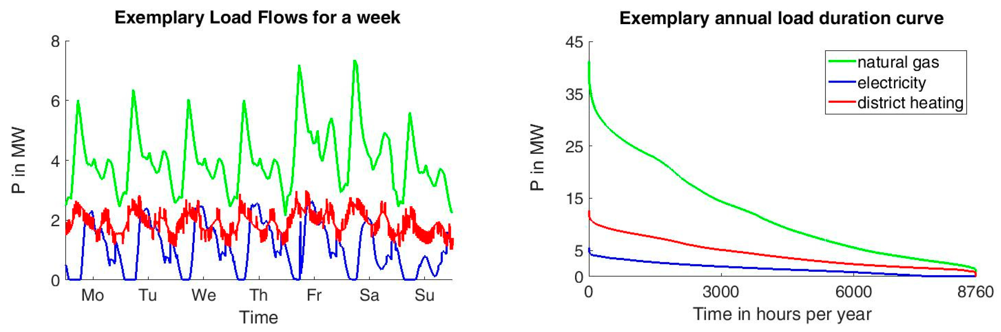
In order to demonstrate the functionality of HyFlow, Figure 11, Figure 12, Figure 13 and Figure 14 aim to provide a better insight on the level of detail that is to be expected for internal elements such as specific power lines, sector coupling—and energy storage utilization. In Figure 11, selected power line of the city in district 1 between cell 5 and cell 18 (see Figure 6) was randomly selected for demonstration purposes. One can see the time-resolved power of all grid-bound energy carriers for a week (left) and as a load duration curve (right). One can see the time-resolved power of all grid-bound energy carriers for a week (left) and as a load duration curve (right).

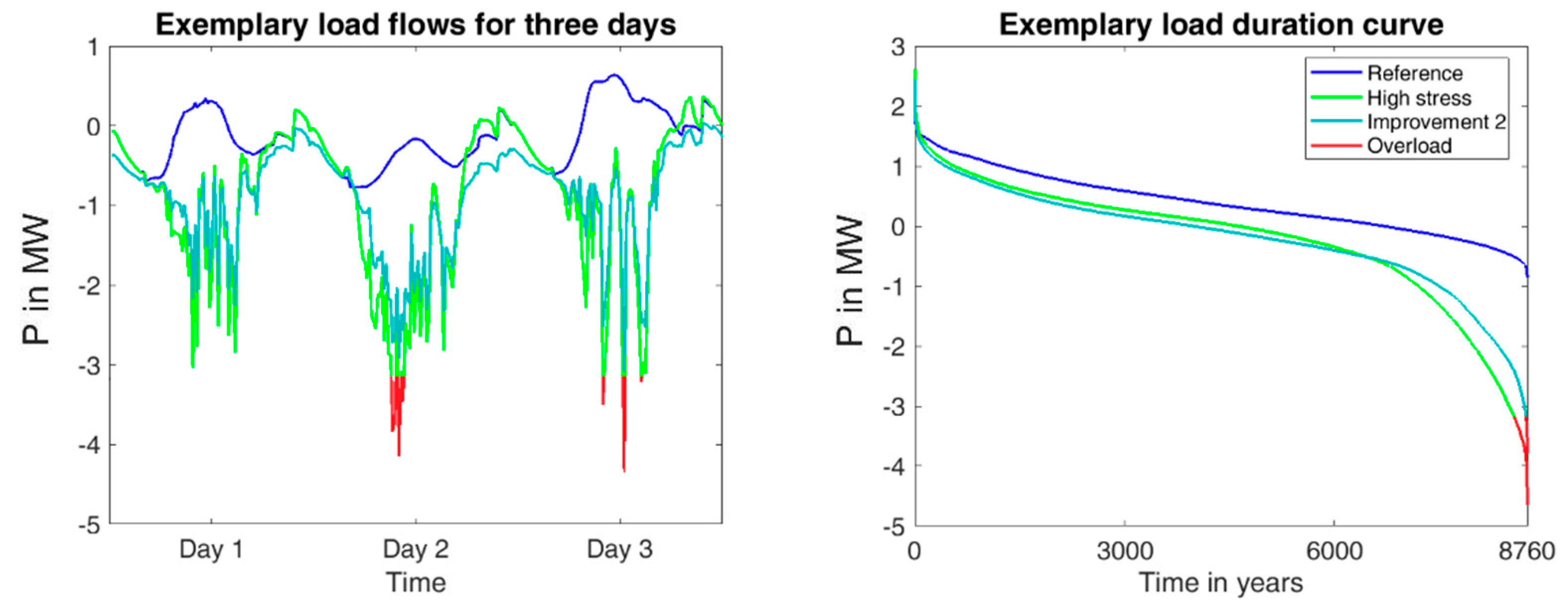
The maximum current carrying capacity I_therm of an electrical power line is dependent on the cable type used. The deciding factors are the nominal voltage and the cross-sectional area of the power line. The maximum power carrying capacity P_therm is therefore defined as I_therm times the nominal voltage. In the case of a chosen power line of the city center (slack node to cell 1—see Figure 6) P_therm amounts to 3.2 MW. One can clearly see the increased negative load flows of the high-stress scenario compared to the reference scenario. At times, where P_therm exceeds the allowed value, the graph for the three exemplary days is marked in red. In the case of the three chosen days, only certain peaks of the high-stress scenario induce overloads on the specific power line. The overall load flow duration curve is shown in the right part of Figure 12. It shows that the chosen measures of improvement scenario 2 helps to reduce the maximum peak power and to reduce the times, where an overload occurs. In the high-stress scenario, the maximum power of the line is 4.65 MW and the overall duration with a registered overload is 176 h in the modeled year. The improvement scenario 2 is not able to prevent all occurring overloads, but helps to reduce them to 18 h per year with an occurring maximum power of 3.8 MW.

Figure 13 shows the utilization profile of the P2G plant in the improvement scenario 2 for a selected week. The P2G plant operates at times of negative residual loads caused by surpluses of the fluctuating renewable generation. Its set maximum power of 500 MW is rarely used (around 26 h per year), but the overall hours of operation amount to more than 2200 h. This high amount of operation is supported by the continuous large demand of natural gas by the industrial cell. If there was a more fluctuating demand profile of natural gas, a gas storage would help to ensure a high utilization rate.

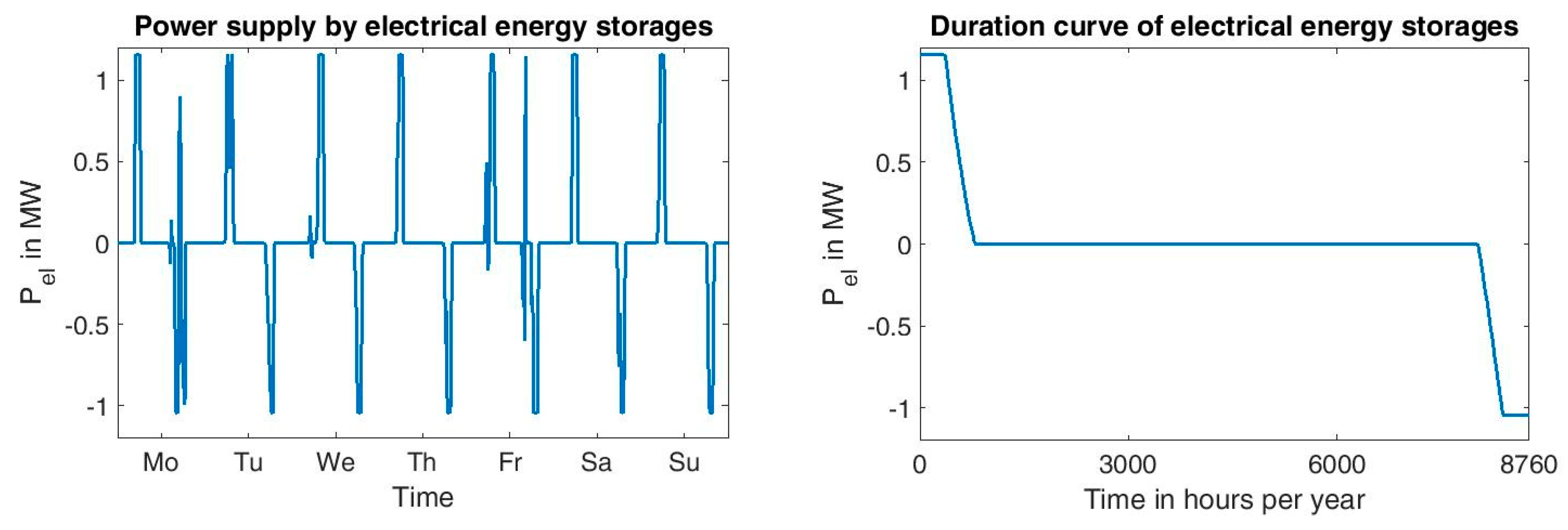
In Figure 14, one can see a charging/discharging profile for a randomly chosen week. The visualization shows that the system serving energy storage units is operated in its maximum power very often and shows a very evenly distributed charging/discharging cycle. The appearance of both visualizations allows us to conclude that only a small share of the positive and negative residual loads can be stored with the energy storage unit. Predominantly, the storage is inactive, because it is either full or empty, which can be seen in the duration curve.

6. Discussion

The methodology of HyFlow has proved to be applicable in a wide range of applications. Combined with the cellular approach described, it allows the user to depict MES and perform load flow calculations in all three grid bound energy carriers. This ensures that expected changes in the energy systems (e.g., more RES, larger amounts of EV) can be evaluated, and that the proposed measures for higher fluctuations (such as energy storages, sector coupling, DSM) are feasible and effective not just for the grid of one energy carrier, but for the total energy system.

The results of the case studies show that the maximum peaks (positive/negative) are expected to increase with the implementation of more fluctuating energy sources of PV and wind and the increase of electromobility. With the usage of measures, such as energy storage and sector coupling technologies, these peaks can be reduced. In particular, the peaks of the negative residual loads and the amount of exported electricity were significantly reduced in the chosen case studies. The use of these negative residual loads also helped to reduce the necessary imports of heat and natural gas, when the according sector-coupling technologies P2G and P2H were available. However, the results for all case studies show, that the imported electricity and the positive peaks of the residual loads of electricity were not significantly reduced with the described measures of the chosen case studies. This effect can only be reached by either a higher generation capacity of electricity or sector-coupling technologies with an output of electricity. There are many challenges and planned improvements in HyFlow. Some examples of currently planned improvements are listed below:

• The integration of more different control strategies for energy storage technologies, based on mathematical optimization algorithms.
• Implementation of an AC load flow calculation methodology to improve accuracy of the modelling framework and consider reactive power as well.
• The adaptation of the district heating load flow calculations is planned. In particular, the heat losses in the heat pipes of flow and return flow need to be integrated.
• An additional tool to evaluate ecological key performance indicators (KPIs) like primary energy efficiency or CO₂ emissions of the chosen scenarios should be included.
• There are plans to improve the usability by introducing a graphical user interface.
• The consideration of uncertainties in the form of a PLF via a Monte Carlo approach.

References

- Mancarella, P. MES (multi-energy systems): An overview of concepts and evaluation models. Energy 2014, 65, 1–17. [Google Scholar] [CrossRef]
- Connolly, D.; Lund, H.; Mathiesen, B.V.; Leahy, M. A review of computer tools for analysing the integration of renewable energy into various energy systems. Appl. Energy 2010, 87, 1059–1082. [Google Scholar] [CrossRef]
- Van Beuzekom, I.; Gibescu, M.; Pinson, P.; Slootweg, J.G. Optimal planning of integrated multi-energy systems. In Proceedings of the 2017 IEEE Manchester PowerTech, Manchester, UK, 18–22 June 2017; pp. 1–6. [Google Scholar]
- Mancarella, P.; Andersson, G.; Pecas-Lopes, J.A.; Bell, K.R.W. Modelling of integrated multi-energy systems: Drivers, requirements, and opportunities. In Proceedings of the 2016 Power Systems Computation Conference (PSCC), Genoa, Italy, 20–24 June 2016; pp. 1–22, ISBN 978-88-941051-2-4. [Google Scholar]
- Hawkes, A.D.; Leach, M.A. Impacts of temporal precision in optimisation modelling of micro-Combined Heat and Power. Energy 2005, 30, 1759–1779. [Google Scholar] [CrossRef]
- Welsch, M.; Mentis, D.; Howells, M. Long-Term Energy Systems Planning. In Renewable Energy Integration; Jones, L.E., Ed.; Elsevier: Amsterdam, The Netherlands, 2014; pp. 215–225. ISBN 9780124079106. [Google Scholar]
- Collins, S.; Deane, J.P.; Poncelet, K.; Panos, E.; Pietzcker, R.C.; Delarue, E.; Gallachóir, B.P.Ó. Integrating short term variations of the power system into integrated energy system models: A methodological review. Renew. Sustain. Energy Rev. 2017, 76, 839–856. [Google Scholar] [CrossRef]
- Van Beuzekom, I.; Gibescu, M.; Slootweg, J.G. A review of multi-energy system planning and optimization tools for sustainable urban development. In Proceedings of the 2015 IEEE Eindhoven PowerTech, Eindhoven, The Netherlands, 29 June–2 July 2015; pp. 1–7. [Google Scholar]
- Good, N.; Zhang, L.; Navarro-Espinosa, A.; Mancarella, P. High resolution modelling of multi-energy domestic demand profiles. Appl. Energy 2015, 137, 193–210. [Google Scholar] [CrossRef]
- Corrado, V.; Fabrizio, E.; Filippi, M. Modelling and optimization of multi-energy source building systems in the design concept phase. In Proceedings of the Clima 2007, WellBeeing Indoors, Helsinki, Finland, 10–14 June 2007. [Google Scholar]
- Lund, H.; Mathiesen, B.V. Energy system analysis of 100% renewable energy systems—The case of Denmark in years 2030 and 2050. Energy 2009, 34, 524–531. [Google Scholar] [CrossRef]
- Pillai, J.R.; Heussen, K.; Østergaard, P.A. Comparative analysis of hourly and dynamic power balancing models for validating future energy scenarios. Energy 2011, 36, 3233–3243. [Google Scholar] [CrossRef]
- Heimberger, M.; Kaufmann, T.; Maier, C.; Nemec-Begluk, S.; Winter, A.; Gawlik, W. Energieträgerübergreifende Planung und Analyse von Energiesystemen. Elektrotech. Inftech. 2017, 134, 229–237. [Google Scholar] [CrossRef]
- Li, F. Spatially Explicit Techno-Economic Optimisation Modelling of UK Heating Futures. Ph.D. Thesis, University College London, London, UK, 2013. [Google Scholar]
- Thiem, S. Multi-Modal On-Site Energy Systems: Development and Application of a Superstructure-Based Optimization Method for Energy System Design under Consideration of Part-Load Efficiencies. Ph.D. Thesis, Technische Universität München, München, Germany, 2017. [Google Scholar]
- Geidl, M.; Koeppel, G.; Perrod, P.F.; Klockl, B.; Andersson, G.; Frohlich, K. Energy hubs for the future. IEEE Power Energy Mag. 2007, 5, 24–30. [Google Scholar] [CrossRef]
- Medjroubi, W.; Müller, U.P.; Scharf, M.; Matke, C.; Kleinhans, D. Open Data in Power Grid Modelling: New Approaches Towards Transparent Grid Models. Energy Rep. 2017, 3, 14–21. [Google Scholar] [CrossRef]
- DIgSILENT GmbH. DIgSILENT PowerFactory; DIgSILENT GmbH: Gomaringen, Germany, 2018. [Google Scholar]
- Siemens AG. PSS SINCAL; Siemens AG: Munich, Germany, 2016. [Google Scholar]
- NEPLAN AG. NEPLAN; NEPLAN AG: Küsnacht, Switzerland, 2018. [Google Scholar]
- Schavemaker, P.; van der Sluis, L. Electrical Power System Essentials; Reprint with corr; Wiley: Chichester, UK, 2009; ISBN 978-0470-51027-8. [Google Scholar]
- Kile, H.; Uhlen, K.; Warland, L.; Kjolle, G. A comparison of AC and DC power flow models for contingency and reliability analysis. In Proceedings of the 2014 Power Systems Computation Conference (PSCC), Wroclaw, Poland, 18–22 August 2014; pp. 1–7, ISBN 978-83-935801-3-2. [Google Scholar]
- Murari, K.; Padhy, N.P. A Network-Topology Based Approach for the Load Flow Solution of AC-DC Distribution System with Distributed Generations. IEEE Trans. Ind. Inform. 2018, 1. [Google Scholar] [CrossRef]
- Fathtabar, H.; Barforoushi, T.; Shahabi, M. Dynamic long-term expansion planning of generation resources and electric transmission network in multi-carrier energy systems. Int. J. Electr. Power Energy Syst. 2018, 102, 97–109. [Google Scholar] [CrossRef]
- Frank, S.; Steponavice, I.; Rebennack, S. Optimal power flow: A bibliographic survey I. Energy Syst. 2012, 3, 221–258. [Google Scholar] [CrossRef]
- Conti, S.; Raiti, S. Probabilistic load flow using Monte Carlo techniques for distribution networks with photovoltaic generators. Sol. Energy 2007, 81, 1473–1481. [Google Scholar] [CrossRef]
- Kabir, M.N.; Mishra, Y.; Bansal, R.C. Probabilistic load flow for distribution systems with uncertain PV generation. Appl. Energy 2016, 163, 343–351. [Google Scholar] [CrossRef]
- Gupta, N. Probabilistic load flow with detailed wind generator models considering correlated wind generation and correlated loads. Renew. Energy 2016, 94, 96–105. [Google Scholar] [CrossRef]
- Ruiz-Rodríguez, F.; Hernández, J.; Jurado, F. Probabilistic Load-Flow Analysis of Biomass-Fuelled Gas Engines with Electrical Vehicles in Distribution Systems. Energies 2017, 10, 1536. [Google Scholar] [CrossRef]
- Pflugradt, N. Modellierung von Wasser- und Energieverbräuchen in Haushalten. Ph.D. Dissertation, Technische Universität Chemnitz, Chemnitz, Germany, 2016. [Google Scholar]
- Almassalkhi, M.; Hiskens, I. Cascade mitigation in energy hub networks. In Proceedings of the 2011 50th IEEE Conference on Decision and Control and European Control Conference, Orlando, FL, USA, 12–15 December 2011; pp. 2181–2188. [Google Scholar]
- Geidl, M.; Andersson, G. Optimal Power Flow of Multiple Energy Carriers. IEEE Trans. Power Syst. 2007, 22, 145–155. [Google Scholar] [CrossRef]
- Liu, X.; Yuan, C.-L.; Liu, X.-Y.; Luo, F.-h.; Feng, Q.; Xu, J.; Chen, G.-H.; Zhou, C.-R. Microstructures, electrical behavior and energy-storage properties of Ba0.06Na0.47Bi0.47TiO3-Ln1/3NbO3 (Ln = La, Nd, Sm) ceramics. Mater. Chem. Phys. 2016, 181, 444–451. [Google Scholar] [CrossRef]
- Kriechbaum, L.; Scheiber, G.; Kienberger, T. Grid-based multi-energy systems—Modelling, assessment, open source modelling frameworks and challenges. Energy Sustain. Soc. 2018, 8, 244. [Google Scholar] [CrossRef]
- Ruiz-Romero, S.; Colmenar-Santos, A.; Mur-Pérez, F.; López-Rey, Á. Integration of distributed generation in the power distribution network: The need for smart grid control systems, communication and equipment for a smart city—Use cases. Renew. Sustain. Energy Rev. 2014, 38, 223–234. [Google Scholar] [CrossRef]
- Kienberger, T.; Böckl, B.; Kriechbaum, L. (Eds.) Hybrid Approaches for Municipal Future Enegy-Grids; IRES: Düsseldorf, Germany, 2016. [Google Scholar]
- Böckl, B.; Kriechbaum, L.; Kienberger, T. Analysemethode für kommunale Energiesysteme unter Anwendung des zellularen Ansatzes. In Proceedings of the EnInnov2016: 14. Symposium Energieinnovation “Energie für unser Europa”—TU Graz, Graz, Österreich, 10–12 February 2016; Institut für Elektrizitätswirtschaft und Energieinnovation, Ed.; ISBN 978-3-85125-448-8. [Google Scholar]
- Gladwin, D.; Todd, R.; Forsyth, A.J.; Foster, M.P.; Strickland, D.; Feehally, T.; Stone, D.A. Battery energy storage systems for the electricity grid: UK research facilities. In Proceedings of the 8th IET International Conference on Power Electronics, Machines and Drives (PEMD 2016), Glasgow, UK, 19–21 April 2016; Institution of Engineering and Technology: Stevenage, UK, 2016; p. 6, ISBN 978-1-78561-188-9. [Google Scholar]
- Vor Dem Esche, R. Benefits of Flywheels for Short Term Grid Stabilisation; Stornetic GmbH: Jülich, Germany, 2017. [Google Scholar]
- Bianchi, M.; Branchini, L.; de Pascale, A.; Peretto, A.; Melino, F.; Orlandini, V. Pump Hydro Storage and Gas Turbines Technologies Combined to Handle Wind Variability: Optimal Hydro Solution for an Italian Case Study. Energy Procedia 2015, 82, 570–576. [Google Scholar] [CrossRef]
- Manchester, S.; Swan, L. Compressed Air Storage and Wind Energy for Time-of-day Electricity Markets. Procedia Comput. Sci. 2013, 19, 720–727. [Google Scholar] [CrossRef]
- Mazhar, A.R.; Liu, S.; Shukla, A. A state of art review on the district heating systems. Renew. Sustain. Energy Rev. 2018, 96, 420–439. [Google Scholar] [CrossRef]
- Yu, H.; Gundersen, T.; Feng, X. Process integration of organic Rankine cycle (ORC) and heat pump for low temperature waste heat recovery. Energy 2018, 160, 330–340. [Google Scholar] [CrossRef]
- Van Hertem, D. Usefulness of DC power flow for active power flow analysis with flow controlling devices. In Proceedings of the 8th IEE International Conference on AC and DC Power Transmission (ACDC 2006), London, UK, 28–31 March 2006; pp. 58–62, ISBN 0 86341 613 6. [Google Scholar]
- Rüdiger, J. Gasnetzsimulation durch Potentialanalyse; Helmut-Schmidt-Universität, Universität der Bundeswehr Hamburg: Hamburg, Germany, 2009. [Google Scholar]
Figure 1.
Visualization of exemplary process steps within the cellular approach.
Figure 2.
Implementation of the cellular approach in HyFlow.
Figure 3.
Implemented hybrid elements in HyFlow.
Figure 4.
Calculation sequence of the HyFlow modelling framework.
Figure 5.
Illustration of the calculation process steps. All red elements are active in the calculation process.
Figure 6.
Topology of case study 1.
Figure 7.
Results of all deployed scenarios of case study 1.
Figure 8.
Topology of case study 2.
Figure 9.
Results of all deployed scenarios of case study 2.
Figure 10.
Load duration curves of energy imports/exports for all energy carriers and one year.
Figure 11.
Exemplary load flows for a selected week on the power line between cell 5 and cell 18 (electricity, natural gas, heat) and the corresponding annual load duration curve.
Figure 12.
Exemplary electrical load flows of the power line Slack-1 in different scenarios.
Figure 13.
Exemplary P2G utilization profile for a chosen week (electrical input power) and the corresponding annual duration curve.
Figure 14.
Exemplary charging/discharging power of a selected electrical energy storage unit and the corresponding annual duration curve.