Assessment of Electric Vehicle Charging Costs in Presence of Distributed Photovoltaic Generation and Variable Electricity Tariffs

Abstract

In this paper a general model for the estimation of the uncoordinated charging costs of Electric Vehicles (EVs) in the presence of distributed and intermittent generation, and variable electricity tariffs is presented. The proposed method aims at estimating the monthly average cost of uncoordinated charging of a single EV depending on the hour at which the EV is plugged into the EV Supply Equipment (EVSE). The feasibility and relevance of the proposed model is verified by applying the considered cost estimation method to a suitable use case. A single EV charging service offered at a public building equipped with a Photovoltaic (PV) system has been considered as reference case. The proposed model has been applied to the PV production and loads consumption data collected during one year, and the results of the study compared with the Time-Of-Use (TOU) electricity tariff. The application of the proposed model identified noticeable deviations among the computed EV charging costs and the reference TOU profile, with differences up to 40%, depending on the considered month and on the time of charging during the day. It can be concluded that such model could be used to properly detect opportunities of energy savings, and to define dedicated EV price signals that could help to promote the optimal use of distributed energy resources.

1. Introduction

The increasing pressure towards decarbonized and sustainable energy systems is heavily affecting the transportation sector, which is progressively called for a radical shift from traditional internal combustion engines (ICEs) towards greener solutions. The growing concerns on the anthropogenic greenhouse gas (GHG) emissions related to the use of road vehicles [1], and on their effect on the air pollution in urban centers [2], are in fact calling for a rapid decarbonization of the urban mobility. From this perspective, electric vehicles (EVs) are generally considered one of the most promising solution, thanks to their independence from the primary energy source, and to the total absence of direct GHG and pollutant emissions. Recent studies demonstrated that the large penetration of EVs could in fact help to significantly reduce both direct and indirect GHG emissions and air pollution in urban areas [3,4]. EVs, in fact, avoid the direct combustion of fossil fuels, and might also help to mitigate the drawbacks caused by intermittent renewable energy sources (RESs), e.g., by potentially acting as storage solutions [5,6,7].

Even though relevant technology developments and rapid cost declines, particularly in the EV battery market, are supporting the prospects of an affordable and effective diffusion of EVs in urban areas, several obstacles are still present, particularly concerning the impact of a large penetration of EVs on the management and operation of existing power networks [8,9,10,11]. Several research streams have recently addressed this concern, by proposing advanced optimization strategies for the integration of EVs in smart grids [12,13,14,15,16,17]. In particular, the application of the Internet of Things (IoT) paradigm and the use of industrial-grade IoT services [18,19] will make available a large amount of information on the use of road vehicles [20], which could be exploited for improving the integration of EVs into smart grids. At the same time, pervasive communication infrastructures, exploiting also the use of power line communication (PLC) systems [21], and of distributed measurement equipment [22], are expected to allow improved observability and enhanced control functions over EV charging networks, including the provisioning of demand response (DR) capabilities.

A particular interest has been paid to the integration and optimization of EV charging processes in the presence of distributed generation (e.g., from photovoltaic and wind power plants), and variable electricity tariffs, by forming the so-called smart charging concept [16]. From this perspective, the smart charging concept, which is usually counterposed to the traditional uncoordinated charging mode, encompasses all of the communication technologies and control strategies which allow the coordinated charging of EVs. In the uncoordinated charging mode, in fact, the power supply provided by the grid to the EVSE depends only on the time of arrival of the EV at the charging station and on the requests of the EV battery charger. Conversely, in the smart charging mode the amount of power provided by the grid and the time of activation of the charging process are controlled by a supervisor, and coordinated with the constraints and operational plans set by distribution grid operators. In Reference [23], for instance, an optimal power flow based optimization framework has been proposed for the coordination of the charging cycles of plug-in hybrid EVs (PHEVs) by minimizing feeder losses and charging costs under time-of-use (TOU) electricity tariffs. In Reference [24], a forecast algorithm for the electrical load of households, based on k-means clustering and an artificial neural network, is used for the optimal scheduling of EV charging in residential applications. In Reference [25], a real-time control strategy for EV charging under dynamic price tariffs is proposed, with the objective of minimizing the charging costs. In Reference [26] a system dynamics (SD) model [27] is proposed to develop a real-time charge pricing mechanism of EVs. In Reference [28] an energy management system is presented to minimize EV charging costs while reducing the energy demand from the grid, and by increasing the self-consumption of Photovoltaic (PV) systems. In Reference [29] a generalized Nash equilibrium problem approach for the management of PHEV charging is presented, by allowing each PHEV to respond price tariff signals to minimize the charging costs, while also considering grid facility constraints.

As suggested by the brief literature review presented above, which represents only an excerpt of the large number of manuscripts published on the matter, the study of advanced EV smart charging strategies has been largely investigated. However, most of the existing works in the literature investigated the topic by mainly focusing on the supervisory control perspective, i.e., by proposing optimal EV charging schedules or variable electricity tariffs with the scope of minimizing the operating cost of the distribution grid. However, even though some of the examined studies took into account the estimation of EV charging costs in coordinated smart grid operations, none of them specifically investigated the modelling of uncoordinated EV charging costs from the prosumers’ perspective in the presence of distributed RES generation and under variable electricity tariffs.

As a matter of fact, most of current EV supply equipment (EVSE), particularly if installed at end-users’ premises (i.e., not for commercial services, such as public charging stations), operates in uncoordinated charging mode. In addition, following the increasing requests of EV charging services at work places or at public buildings, private companies and public administrations have to deal with the proper evaluation of the operating costs related to the requested services, particularly in the presence of distributed RESs, which typically causes both seasonal and intraday variations of prosumers’ energy flows. The aim of the study is thus to provide a general model for the estimation of the uncoordinated charging costs of EVs in presence of distributed and intermittent generation, and variable electricity tariffs. The proposed method aims at estimating the monthly average cost of a single EV uncoordinated charging depending on the hour at which the EV is plugged into the EVSE.

The remainder of the paper is organized as follows: In Section 2, the mathematical definition of the cost estimation method is described in detail, by defining all of the system variables and parameters of the model. Afterwards, the feasibility and relevance of the proposed model is verified by applying the presented cost estimation method to a suitable use case, and by comparing the results of the study with the TOU tariff applied to the energy purchased from the grid. In this study, the evaluation of the operating costs of a single EV charging service offered at a public building equipped with a PV system has been considered as reference case, by applying the proposed model to the PV production and loads consumption data collected during one year. The detailed description of the use case is provided in Section 3. In particular, in Section 3.1 the description of the use case is provided by introducing the main characteristics of the system, and by defining the operation parameters and simulation constraints. In Section 3.2 the PV production and loads consumption data used for the simulation are presented and briefly discussed, while the simulation parameters are defined in Section 3.3. The results of the simulation are then discussed in Section 4, and the conclusion of the study are finally presented in Section 5.

2. Method

The proper evaluation of the charging cost of EVs must take into account all the energy costs related to the considered process, namely: the direct costs due to the increase of energy consumption from the grid, the loss of revenues due to the decrease of the amount of energy sold to the grid, and the costs related to the increase of the demand charge from the utility.

The average cost of an EV uncoordinated charging cycle starting at hour $s$ of month $m$, ${\overline{C}}_{s,m}^{\mathrm{EV}}$, can be computed as follows:

$${\overline{C}}_{s,m}^{\mathrm{EV}}=\frac{{\overline{C}}_{s,m}^{\Delta P_{\mathrm{FU}}}+{\overline{C}}_{s,m}^{\Delta E_{\mathrm{FU}}}+{\overline{C}}_{s,m}^{\Delta E_{\mathrm{TU}}}}{E_{s,m}^{\mathrm{EV}}},$$

(1)

where ${\overline{C}}_{s,m}^{\Delta P_{\mathrm{FU}}}$ is the term due to the increase of the demand charge from the utility related to the specific EV charging cycle starting at hour $s$ of month $m$, ${\overline{C}}_{s,m}^{\Delta E_{\mathrm{FU}}}$ is the term related to the increase of energy consumption from the grid, ${\overline{C}}_{s,m}^{\Delta E_{\mathrm{TU}}}$ is the loss of revenues due to the decrease of the amount of energy sold to the utility (which corresponds to the increase of self-consumed energy due to the specific EV charging cycle), and $E_{s,m}^{\mathrm{EV}}$ is the expected energy consumption of the EV charging cycle starting at hour $s$ of month $m$.

The term ${\overline{C}}_{s,m}^{\Delta P_{\mathrm{FU}}}$ is computed as follows:

$${\overline{C}}_{s,m}^{\Delta P_{\mathrm{FU}}}=\frac{T_m^{P_{\mathrm{FU}}}\Delta P_{s,m}^{\mathrm{FU},\mathrm{EV}}}{n_{s,m}{\sum }_s\Delta P_{s,m}^{\mathrm{FU},\mathrm{EV}}},$$

(2)

where:

• $\Delta P_{s,m}^{\mathrm{FU},\mathrm{EV}}$ is the increase of the demand charge from the utility during month $m$, due to the EV charging cycle starting at hour $s$, expressed in kW;
• $T_m^{P_{\mathrm{FU}}}$ is the cost of the demand charge from the utility during month $m$, expressed as €/kW;
• $n_{s,m}$ is the number of charging cycles starting at hour $s$ during month $m$;

In particular, the term $\Delta P_{s,m}^{\mathrm{FU},\mathrm{EV}}$ is computed as follows:

$$\Delta P_{s,m}^{\mathrm{FU},\mathrm{EV}}={\max }_{i,d}\{P_{i,d,m,s}^{\mathrm{FU},\mathrm{EV}}\}-{\max }_{i,d}\{P_{i,d,m}^{\mathrm{FU}}\},$$

(3)

where $P_{i,d,m,s}^{\mathrm{FU},\mathrm{EV}}$ and $P_{i,d,m}^{\mathrm{FU}}$ are the average value of power absorbed from the utility for each $i$-th time interval of 15 min during the $d$-th day of month $m$, for an EV charging cycle starting at hour $s$, and for the reference case, respectively.

It must be noted that the term ${\overline{C}}_{s,m}^{\Delta P_{\mathrm{FU}}}$ is computed taking into account the weight of the increase of power from the utility due to the EV charging cycle occurring at hour $s$, with respect to the sum of the increases of power due to each simulated charging cycle. In this way, the overall cost related to the increase of the demand charge of the system can be distributed to each charging cycle, depending on its specific contribution to that cost.

The term ${\overline{C}}_{s,m}^{\Delta E_{\mathrm{FU}}}$ is computed as follows:

$${\overline{C}}_{s,m}^{\Delta E_{\mathrm{FU}}}=\frac{{\sum }_{d=1}^{d_m}{\sum }_{h=0}^{23}(T_{h,m}^{E_{\mathrm{FU}}}\Delta E_{h,d,m,s}^{\mathrm{FU},\mathrm{EV}})}{n_{s,m}},$$

(4)

where:

• $T_{h,m}^{E_{\mathrm{FU}}}$ is the cost of electricity absorbed from the grid during hour $h$ of month $m$ (€/kWh);
• $d_m$ is the number of days of month $m$;
• $\Delta E_{h,d,m,s}^{\mathrm{FU},\mathrm{EV}}$ is the increase of the energy consumption from the grid (expressed in kWh) during hour $h$ of the $d$-th day of month $m$, for an EV charging cycle starting at hour $s$. In particular, $\Delta E_{h,d,m,s}^{\mathrm{FU},\mathrm{EV}}$ is computed as follows:

  $$\Delta E_{h,d,m,s}^{\mathrm{FU},\mathrm{EV}}=E_{h,d,m,s}^{\mathrm{FU},\mathrm{EV}}-E_{h,d,m}^{\mathrm{FU}},$$

  (5)

  where $E_{h,d,m,s}^{\mathrm{FU},\mathrm{EV}}$ and $E_{h,d,m}^{\mathrm{FU}}$ are the values of energy absorbed from the grid during hour $h$ of the $d$-th day of month $m$, for an EV charging cycle starting at hour $s$, and for the reference case, respectively.

The term ${\overline{C}}_{s,m}^{\Delta E_{\mathrm{TU}}}$ is computed as follows:

$${\overline{C}}_{s,m}^{\Delta E_{\mathrm{TU}}}=\frac{{\sum }_{d=1}^{d_m}{\sum }_{h=0}^{23}(T_{h,m}^{E_{\mathrm{TU}}}\Delta E_{h,d,m,s}^{\mathrm{TU},\mathrm{EV}})}{n_{s,m}},$$

(6)

where:

• $T_{h,m}^{E_{\mathrm{TU}}}$ is the price of electricity sold to the grid during hour $h$ of month $m$, expressed in €/kWh;
• $\Delta E_{h,d,m,s}^{\mathrm{TU},\mathrm{EV}}$ is the decrease of the energy injected to the grid (expressed in kWh) during hour $h$ of the $d$-th day of month $m$, for an EV charging cycle starting at hour $s$. In particular, $\Delta E_{h,d,m,s}^{\mathrm{TU},\mathrm{EV}}$ is computed as follows:

  $$\Delta E_{h,d,m,s}^{\mathrm{TU},\mathrm{EV}}=E_{h,d,m}^{\mathrm{TU}}-E_{h,d,m,s}^{\mathrm{TU},\mathrm{EV}},$$

  (7)

  where $E_{h,d,m,s}^{\mathrm{TU},\mathrm{EV}}$ and $E_{h,d,m}^{\mathrm{TU}}$ are the values of energy injected into the grid during hour $h$ of the $d$-th day of month $m$, for an EV charging cycle starting at hour $s$, and for the reference case, respectively.

3. Use Case

In the present study, the evaluation of the operating costs of a single EV charging service offered at a public building located in the engineering campus of the University of Brescia, Italy, and equipped with a 64 kWp PV system, has been considered as reference use case. A brief description of the system and the definition of the operation parameters and simulation constraints of the simulated EV charging service are described in Section 3.1. The estimation of the EV charging costs for the considered case is carried out by applying the proposed model to the PV production and loads consumption data collected during 2017, as discussed in Section 3.2. In this study, it is assumed that a single point EV charging service is offered to the public during the opening hours of the building. The service calendars and EV charging profile used for the simulation are finally described in Section 3.3.

3.1. Description of the Use Case System

A public building located in the engineering campus of the University of Brescia, Italy, has been chosen as reference use case. The building includes both department facilities (i.e., offices and classrooms), and student services, comprising dormitories, study halls, a cafeteria, a gym, and a baseball field. The building is connected to the local low voltage (LV) distribution grid, and is equipped with a 64 kWp PV system.

In this study, it is assumed that a single point EVSE is installed at the LV point of delivery (POD) of the system, and that an EV charging service is offered publicly during the opening hours of the building. In this case, the results of the simulation are expected to provide useful information to the energy and facility manager of the University, by estimating the operating costs of the proposed EV charging service, by taking into consideration the variability and intermittency of the PV power generation, and the energy consumption of the building. Such information could be, for instance, compared to the current electricity tariffs applied by the local energy retailer, and then used to better estimate the price that must be charged to final users, depending on the time of EV charging.

3.2. PV Production and Loads Consumption Data

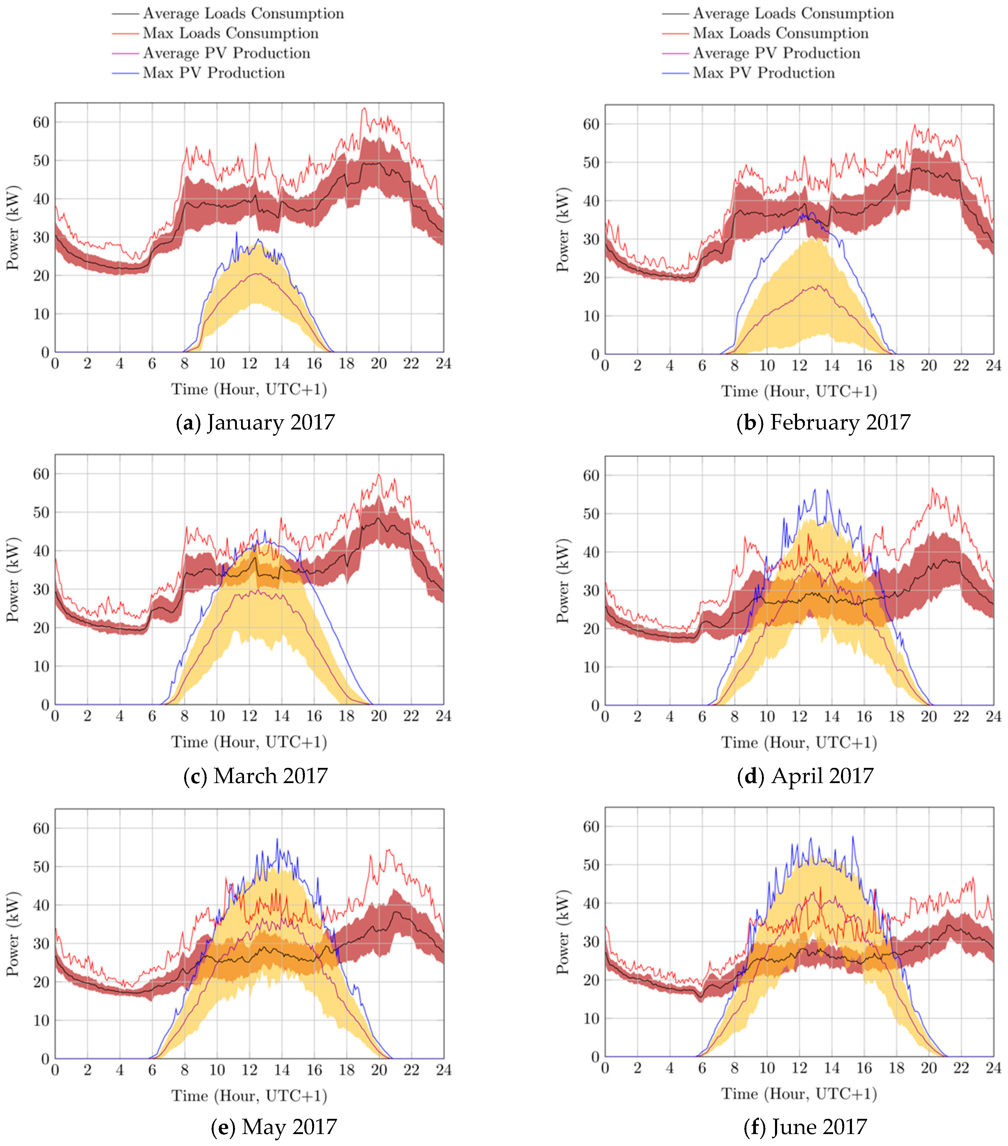
In the following, the PV production and loads consumption data used for the simulation are briefly introduced, by presenting the monthly average and peak power data of the PV production and of user’s loads consumption recorded from January to June 2017, and from July to December 2017, as depicted in Figure 1 and Figure 2, respectively.

The presented monthly average and peak data are computed from a set of data recorded every 5 min. Each of the recorded value is computed as the average of data sampled every 10 s. The yellow and red area represent the standard deviation of the measured PV power production and of the measured loads power consumption, respectively. Further information on the measurement system used to collect the herein presented data is provided in Reference [30].

As it can be observed by the graphs of Figure 1 and Figure 2, the power consumption profile of loads shows a typical behavior during almost all the months of the year, by forming a sort of “reverse tilde” shape. The power demand of loads reaches its maximum value among 8 and 9 p.m. (with monthly averages ranging from 26.4 to 50.5 kW), and then rapidly decreases up to 1 am, by afterwards slowly reaching its minimum around 4 and 6 a.m. in the morning (with monthly averages ranging from 15.4 to 26.3 kW). After 6 a.m. in the morning, the power consumption rapidly increases up to 8 a.m., by then remaining almost constant up to 4 p.m. in the afternoon, and then by further increasing to reach the peak around 8 and 9 p.m. It must be also noted that this particular shape is generally replicated each month, with only few differences during July and August (apparently due to summer vacations), where the power consumption profile shows a sort of flattening, i.e., a reduction between peaks and valleys. Moreover, the typical shape of the daily power consumption profile also reveals a sort of “drift” effect during the year, by progressively showing a global down shift from January to August, and then a global up shift from September to December. Finally, it can also be observed that also the computed standard deviation of the mean shows noticeable variations depending on the time of the day and on the considered month. Generally, it can be noted that, for each observed month, the power demand profile seems quite stable, i.e., by showing very small deviations (ranging from 0.5 to 2.6 kW), while during peaks, or during months characterized by unstable weather conditions (such as April), the standard deviation of the average power consumption can be very high, by ranging from 5.1 to 8.9 kW.

Data depicted in Figure 1 and Figure 2 also show that, as expected, the power production of the PV system exhibits the typical daily and seasonal variations during the year, and that its standard deviation is noticeably greater than that of loads. The comparison between the PV and loads power profiles also reveals that during months characterized by high solar radiation (i.e., from April to September), the PV production may be greater than the loads consumption, thus producing reverse power flows into the grid.

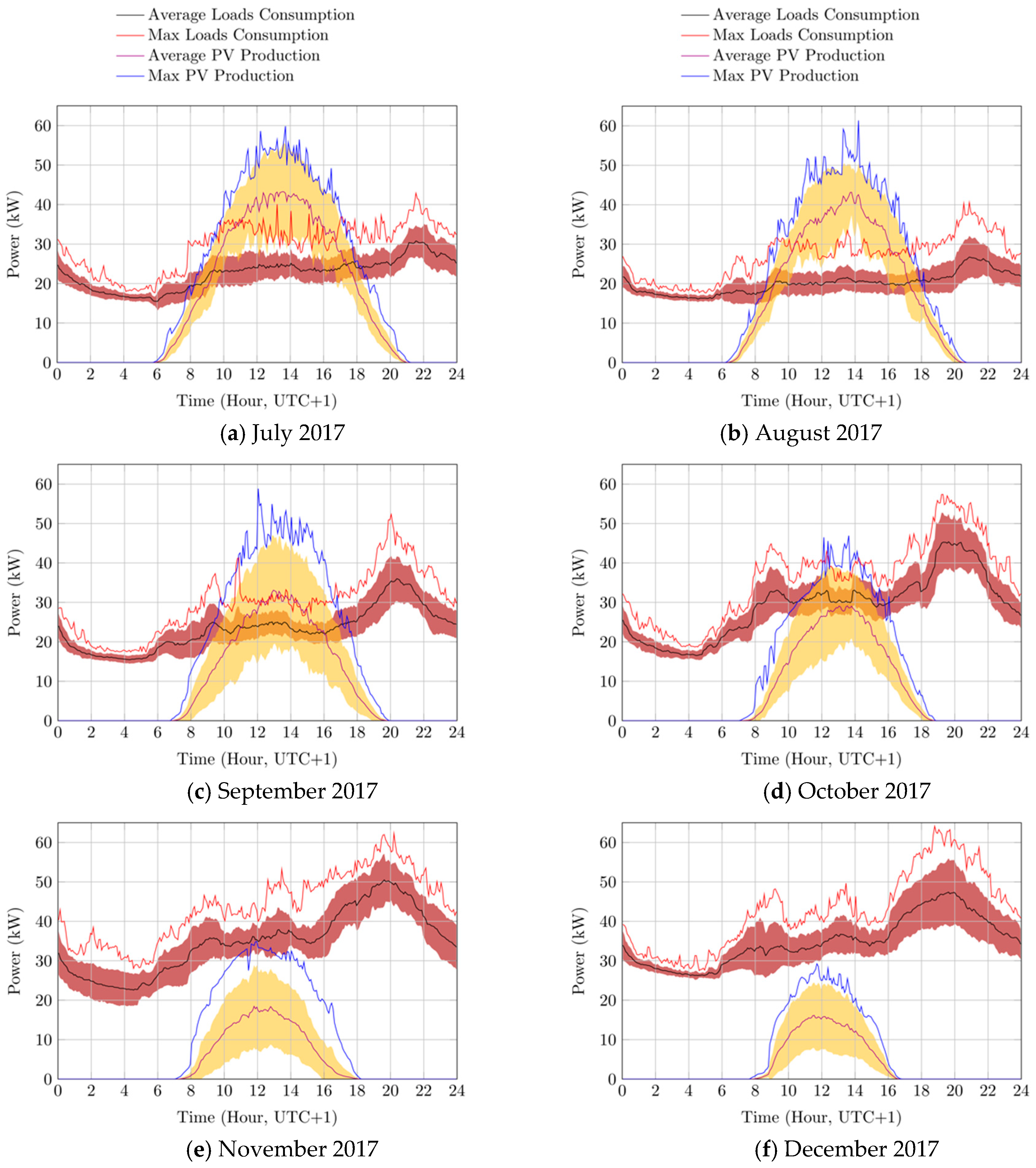
The power balance at the user’s POD has been then computed for each 5 min time interval, by taking into account the power consumption of the loads and the PV production, and the monthly average, standard deviation, and peak values have been plotted for each month, from January to June 2017, and from July to December 2017, as depicted in Figure 3 and Figure 4, respectively.

The maximum power consumption from the grid is computed for each time interval of 15 min, and then used to determine the monthly charged power from the utility (i.e., equal to the highest value of all of the computed 15 min maximum values).

As it can be observed by the graphs depicted in Figure 3 and Figure 4, the power profile at the user’s POD shows a typical “tilted S” shape, which results from the combination of the typical profiles of the loads consumption and of the PV production. In particular, it can be noted that the computed standard deviations of the power flows at the user’s POD are noticeably greater than that of user’s loads, with highest monthly values ranging from 10.4 to 17.4 kW, while the same values recorded by user’s loads rage from 5.1 to 8.9 kW. This is apparently due to the variability and uncertain production of the PV system, which causes relevant disturbances to the power flows measured at the user’s POD.

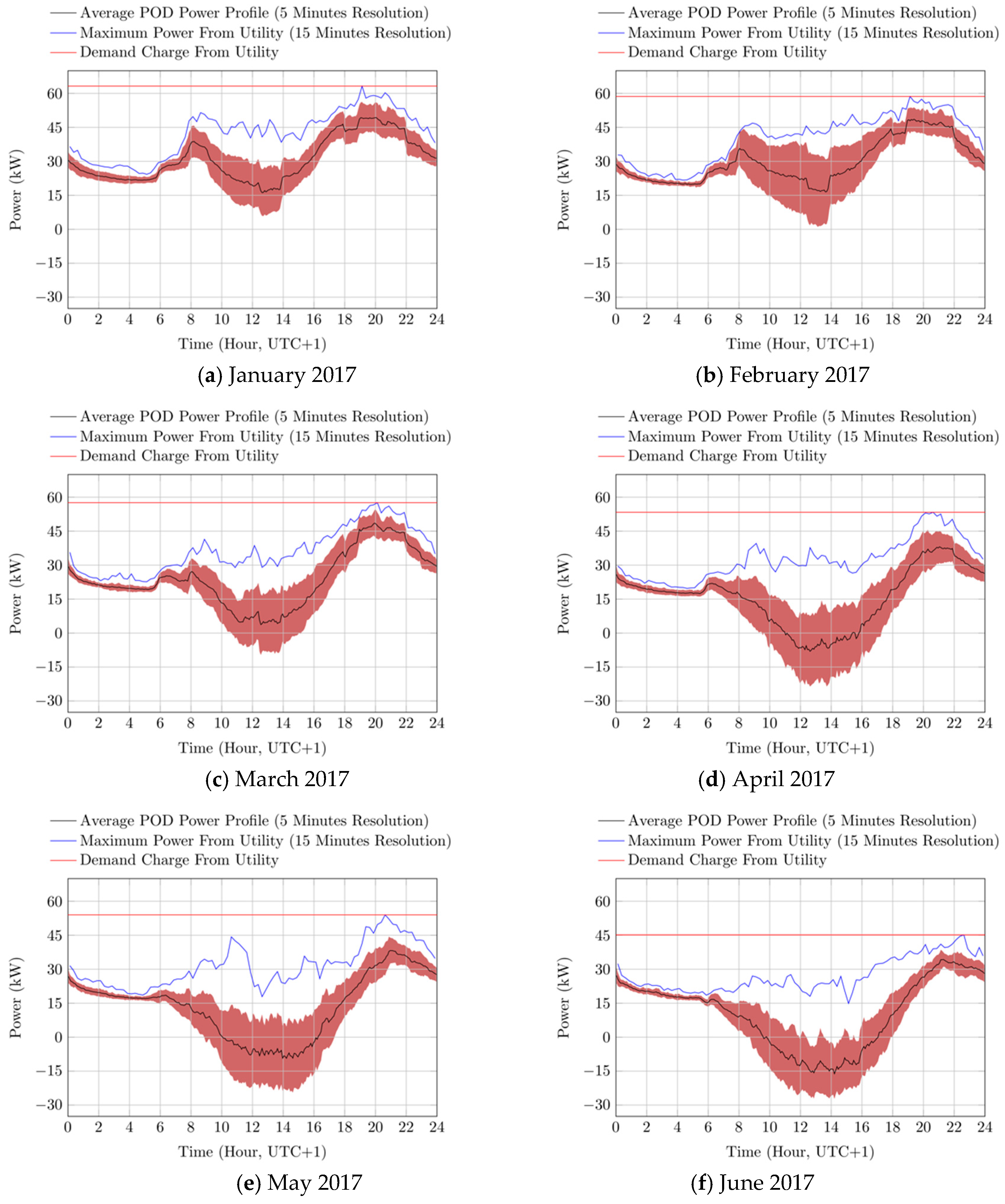
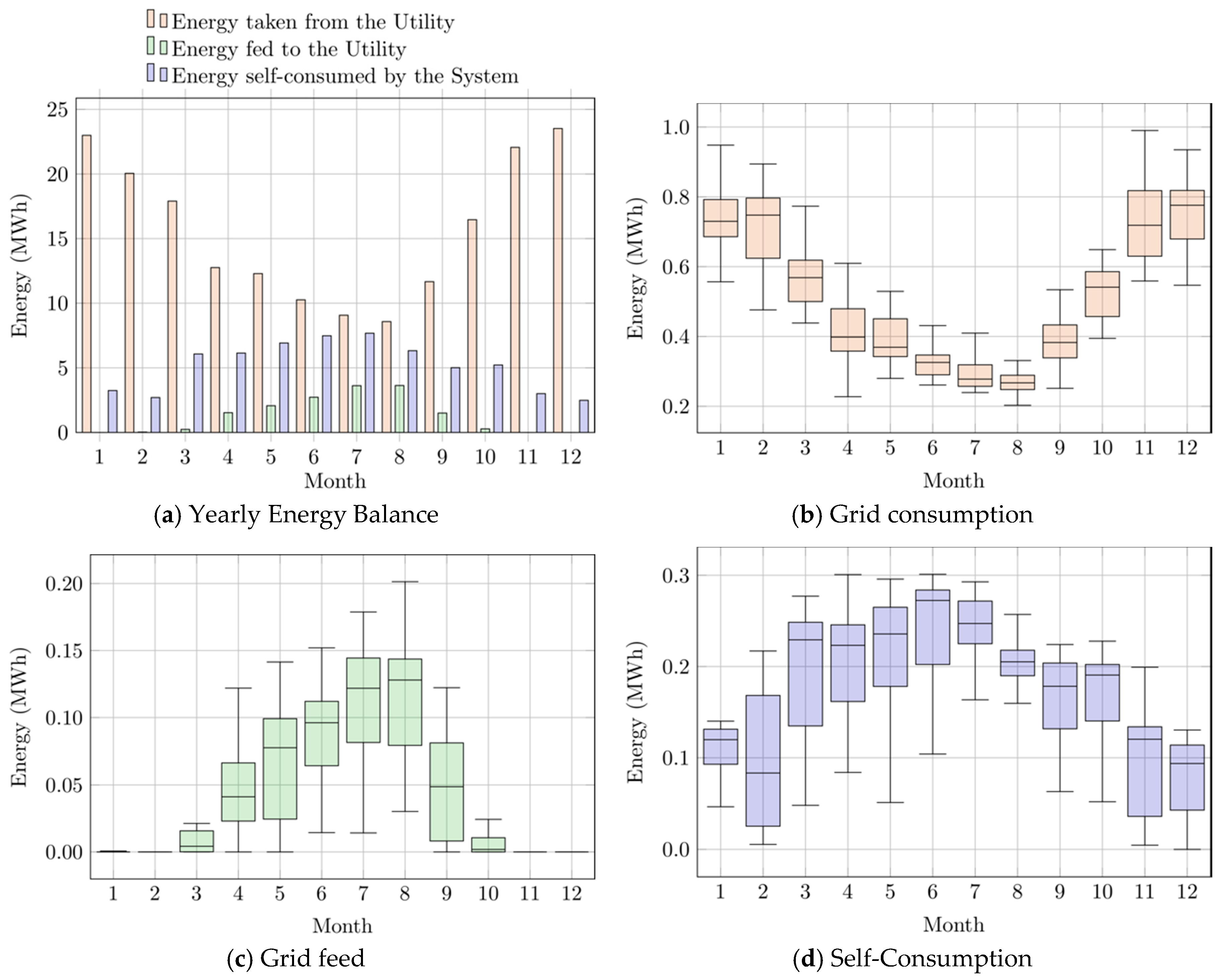
The monthly and yearly energy balance of the system is then computed based on all of the data recorded during 2017 every 5 min, as depicted in Figure 5. In sub-figure (a) the monthly energy flows of the system are reported for each month, by specifying the amount of energy absorbed from the grid, injected into the grid, and self-consumed by the system (i.e., produced by the photovoltaic system and consumed by the user’s loads). In sub-figures (b), (c), and (d), the interquartile analyses of the daily energy absorbed from the grid, injected into the grid, and self-consumed by the system are reported for each month, respectively.

If we look at charts of Figure 5, it can be noted that the amount of energy absorbed from the utility decreases from January to August, and then increases during the following months, with values ranging from 8.6 MWh to 23.5 MWh. Conversely, the amount of energy injected into the utility, due to the overproduction of the PV system, and the amount of self-consumed energy increase from January to August, and then decrease during the following months, with values raging from almost zero to 3.6 MWh, and from 2.5 MWh to 7.7 MWh, respectively.

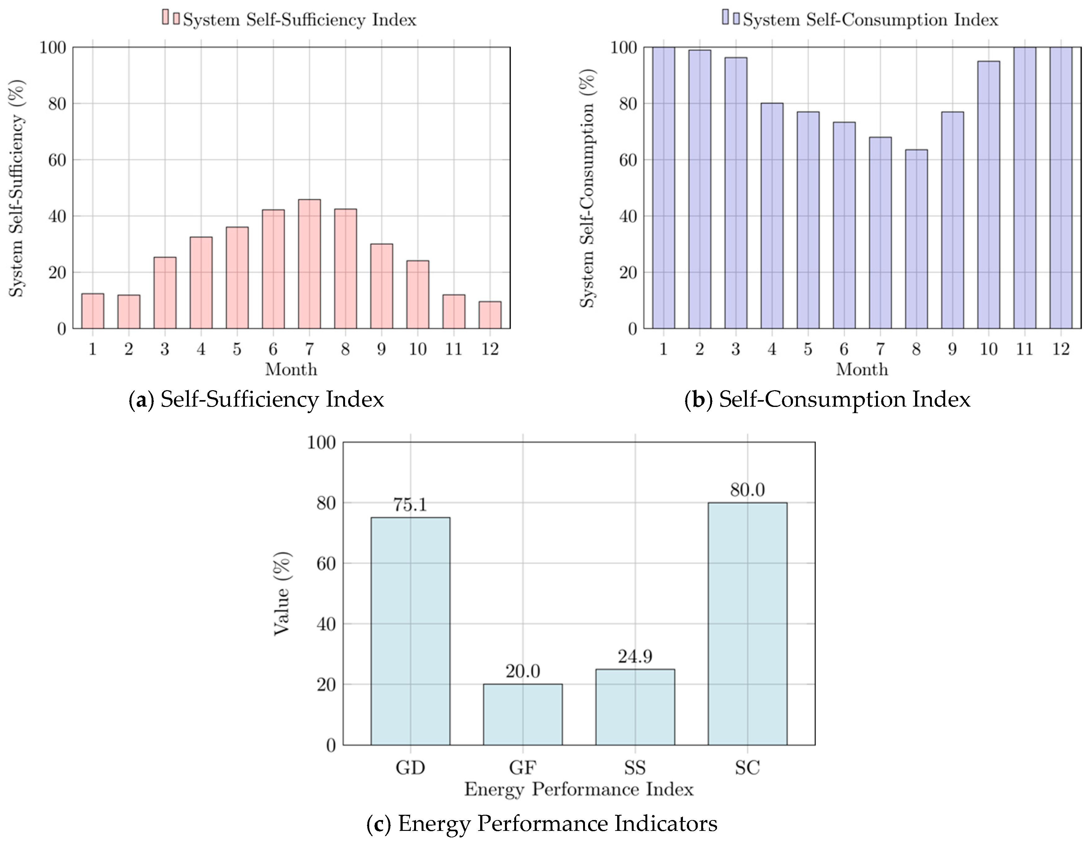
Finally, the energy key performance indicators (KPIs) of the system have been computed, based on data measured during 2017, as shown in Figure 6. In subfigures (a) and (b) the self-sufficiency and the self-consumption of the system are reported for each month, respectively. In sub-figure (c), the Grid-Dependency (GD), Grid-Feed (GF), Self-Sufficiency (SS), and Self-Consumption (SC) indices are reported.

The self-sufficiency index of the system estimates the independency of the system from the power grid and is computed as the ratio between the energy provided by the PV to loads, and the overall loads consumption. In particular, the self-sufficiency index can be computed as follows:

$${\mathrm{SS}}_m=\frac{{\sum }_{d=1}^{d_m}{\sum }_i\min \{{\overline{P}}_{i,d,m}^{\mathrm{PV}},{\overline{P}}_{i,d,m}^{\mathrm{L}}\}\Delta t}{{\sum }_{d=1}^{d_m}{\sum }_i{\overline{P}}_{i,d,m}^{\mathrm{L}}\Delta t},$$

(8)

where:

• ${\mathrm{SS}}_m$ is self-sufficiency index of month $m$;
• ${\overline{P}}_{i,d,m}^{\mathrm{PV}}$ and ${\overline{P}}_{i,d,m}^{\mathrm{L}}$ are the average power produced by the PV system and consumed by the user’s loads during the $i$-th time interval of day $d$ of month $m$, respectively;
• $\Delta t$ is the duration of the considered time interval.

The self-consumption index estimates the amount of energy produced by the PV plant, which is directly consumed by the system loads, and is computed as the ratio between the energy provided by the PV to loads, and the overall PV production. In particular, the self-consumption index can be computed as follows:

$${\mathrm{SC}}_m=\frac{{\sum }_{d=1}^{d_m}{\sum }_i\min \{{\overline{P}}_{i,d,m}^{\mathrm{PV}},{\overline{P}}_{i,d,m}^{\mathrm{L}}\}\Delta t}{{\sum }_{d=1}^{d_m}{\sum }_i{\overline{P}}_{i,d,m}^{\mathrm{PV}}\Delta t},$$

(9)

where ${\mathrm{SC}}_m$ is self-consumption index of month $m$.

The grid-dependency index estimates the dependency of the user’s loads from the grid and is computed as the ratio between the grid consumption and the overall loads consumption. In particular, the grid-dependency index can be computed as follows:

$${\mathrm{GD}}_m=\frac{{\sum }_{d=1}^{d_m}{\sum }_i{\overline{P}}_{i,d,m}^{\mathrm{FU}}\Delta t}{{\sum }_{d=1}^{d_m}{\sum }_i{\overline{P}}_{i,d,m}^{\mathrm{L}}\Delta t},$$

(10)

where:

• ${\mathrm{GD}}_m$ is grid-dependency index of month $m$;
• ${\overline{P}}_{i,d,m}^{\mathrm{FU}}$ is the average power absorbed from the grid by the user’s loads during the $i$-th time interval of day $d$ of month $m$.

Finally, the grid-feed index estimates the overproduction ratio of the PV system and is computed as the ratio between the energy injected into the grid by the PV system, and the overall PV production. In particular, the grid-feed index can be computed as follows:

$${\mathrm{GF}}_m=\frac{{\sum }_{d=1}^{d_m}{\sum }_i{\overline{P}}_{i,d,m}^{\mathrm{TU}}\Delta t}{{\sum }_{d=1}^{d_m}{\sum }_i{\overline{P}}_{i,d,m}^{\mathrm{PV}}\Delta t},$$

(11)

where:

• ${\mathrm{GF}}_m$ is grid-feed index of month $m$;
• ${\overline{P}}_{i,d,m}^{\mathrm{TU}}$ is the average power injected into the grid by the PV system during the $i$-th time interval of day $d$ of month $m$.

3.3. Simulation Parameters

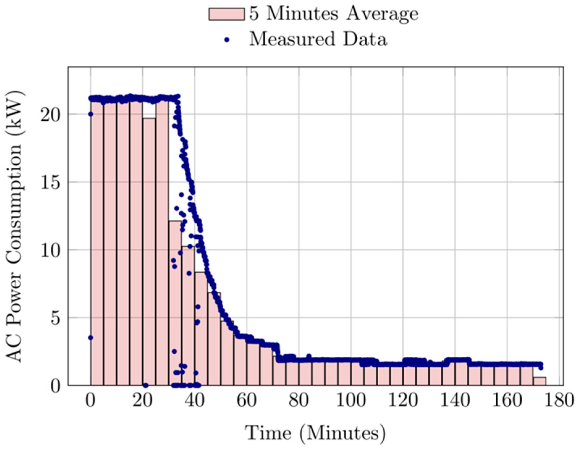
In this study, a typical EV charging power profile is assumed as reference charging cycle. The considered EV charging profile, depicted in Figure 7, was measured during a real charging process of a commercial EV (Renault ZOE), with an initial state of charge (SOC) of 35%, up to a 100% SOC.

A three-phase power meter UPM209 produced by Algodue Elettronica s.r.l. (Maggiora, Italy), equipped with a Rogowski coil current transducer, was used to measure the power consumption of the EVSE, while the EV SOC was measured by accessing the on-board diagnostic (OBD) system of the EV. Further details on system used for the power and EV SOC measurements can be found in [31].

The set of EV charging cycles considered in the simulation are defined by the charging calendar reported in

Table 1. Charging calendar considered in the present study. Days where the EV charging service is available are represented by 1, and by 0 otherwise. EV: Electric Vehicle.

Day/Month	1	2	3	4	5	6	7	8	9	10	11	12
1	0	1	1	0	0	1	0	1	1	0	0	1
2	0	1	1	0	1	0	0	1	0	1	1	0
3	0	1	1	1	1	0	1	1	0	1	1	0
4	0	0	0	1	1	0	1	1	1	1	0	1
5	0	0	0	1	1	1	1	0	1	1	0	1
6	0	1	1	1	0	1	1	0	1	1	1	1
7	0	1	1	1	0	1	1	1	1	0	1	1
8	0	1	1	0	1	1	0	1	1	0	1	0
9	1	1	1	0	1	1	0	1	0	1	1	0
10	1	1	1	1	1	0	1	1	0	1	1	0
11	1	0	0	1	1	0	1	1	1	1	0	1
12	1	0	0	1	1	1	1	0	1	1	0	1
13	1	1	1	1	0	1	1	0	1	1	1	1
14	0	1	1	1	0	1	1	0	1	0	1	1
15	0	1	1	0	1	1	0	0	1	0	1	1
16	1	1	1	0	1	1	0	0	0	1	1	0
17	1	1	1	0	1	0	1	0	0	1	1	0
18	1	0	0	1	1	0	1	0	1	1	0	1
19	1	0	0	1	1	1	1	0	1	1	0	1
20	1	1	1	1	0	1	1	0	1	1	1	1
21	0	1	1	1	0	1	1	1	1	0	1	1
22	0	1	1	0	1	1	0	1	1	0	1	1
23	1	1	1	0	1	1	0	1	0	1	1	0
24	1	1	1	0	1	0	1	1	0	1	1	0
25	1	0	0	0	1	0	1	1	1	1	0	0
26	1	0	0	1	1	1	1	0	1	1	0	0
27	1	1	1	1	0	1	1	0	1	1	1	0
28	0	1	1	1	0	1	1	1	1	0	1	0
29	0	-	1	0	1	1	0	1	1	0	1	0
30	1	-	1	0	1	1	0	1	0	1	1	0
31	1	-	1	-	1	-	1	1	-	1	-	0

. The table defines, for each day of each month of 2017, the availability of the charging service to the public. Days where the EV charging service is available are represented by 1, and by 0 otherwise. The calendar was defined by taking into consideration the weekly opening days of the building, and the national and local holidays. In particular, considering that the daily opening hours of the buildings are from 8 a.m. to 8 p.m., and that the assumed EV charging cycle time is of about 3 h, in this study it is assumed that the EV charging initial time $s$ may range from 8 a.m. to 5 p.m.

Even though variable tariff profiles can be applied in the proposed model, for both the energy purchased from the grid and the energy sold to the grid, constant tariff components have been considered in the present study. In particular, a rated power cost ($T_m^{P_{\mathrm{FU}}}$) of 5 €/kW per month was considered for the monthly power peak from the grid, while 0.18 €/kWh and 0.1 €/kWh was set as energy consumption tariff ($T_m^{E_{\mathrm{FU}}}$) and energy feed tariff ($T_m^{E_{\mathrm{TU}}}$), respectively. The use of constant tariff components has been chosen to better evaluate the benefits of the proposed model for the estimation of the EV charging cost, with respect to the use of the energy prices applied by the utility.

4. Results and Discussion

The average cost of the EV uncoordinated charging starting at hour $s$ for each month $m$, ${\overline{C}}_{s,m}^{\mathrm{EV}}$, was computed by using the measured loads consumption and PV production data described in Section 3. For each day of month $m$, and for each hour $s$, an EV charging process starting at hour $s$ was simulated by adding the EV charging power profile to the measured loads power profile. The simulated POD power profile was then built by taking into account the measured PV power production, and the related monthly average charging cost was computed according to the model described in Section 2. The simulation has been implemented by means of a dedicated C++ code.

In the following, the results of the simulation are presented and discussed in detail.

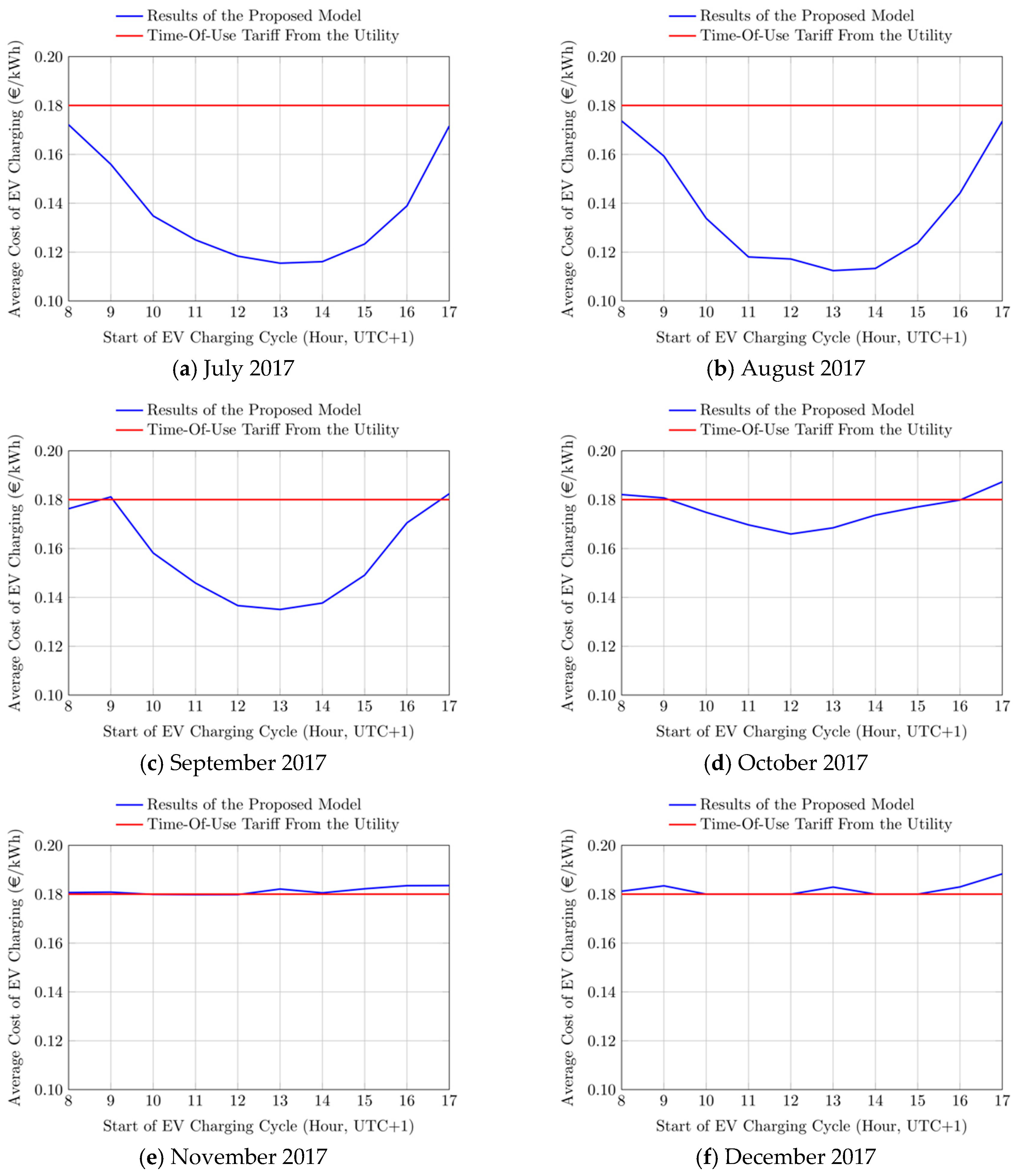
In Figure 8 and Figure 9, the computed monthly average cost of EV charging (reported as €/kWh) from January to June 2017, and from July to December 2017 are reported, respectively. The computed EV charging cost for each hour (i.e., depending on the time of arrival of the EV at the charging station), represented with the blue line, is compared to the time-of-use (TOE) electricity tariff applied to the amount of energy purchased from the grid (red line).

The results show that the EV charging costs computed by the proposed model may noticeably differ from the reference TOU profile, depending on the considered month and on the time of charging during the day. In particular, it can be noted that during seasons characterized by low PV production (i.e., from October to March), the computed EV charging cost is very close or equal to the TOU tariff applied by the utility to the amount of energy purchased by the grid. Only during early morning and late afternoon hours the computed EV charging cost is slightly higher than the TOU tariff, due to the sensible increase of rated power demand from the utility.

Conversely, during seasons with higher PV production (i.e., from April to September), the computed EV charging cost noticeably differ from the TOU tariff, particularly during late mornings and early afternoons, where the PV production reaches its higher values. It must be also noted that the highest reported difference (occurring at 1 p.m. in August) is on the order of 0.07 €/kWh, which corresponds to a difference of 1.24 € per each EV charging cycle, thus representing a possible estimated saving of about 40% with respect the considered TOU tariff.

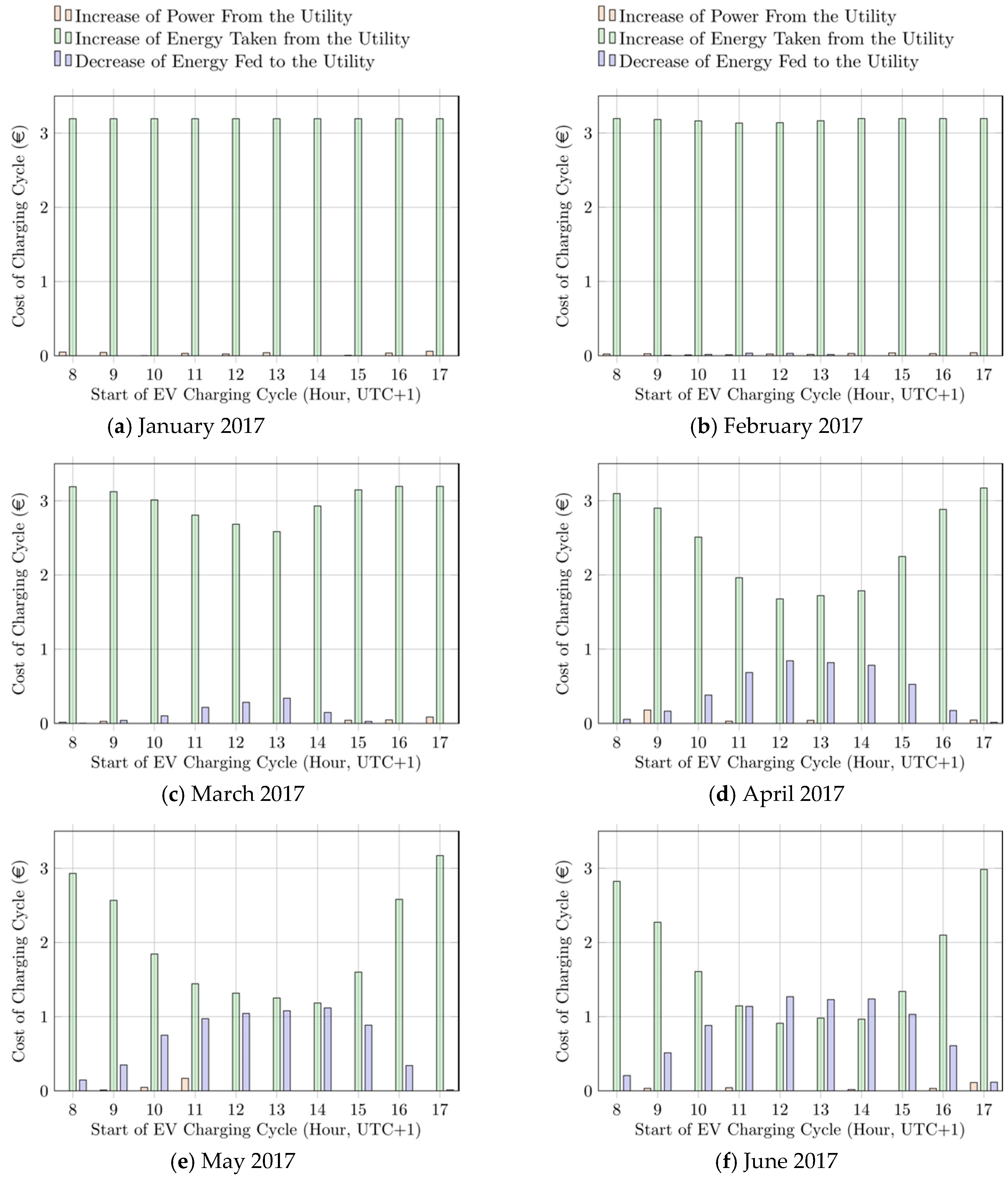
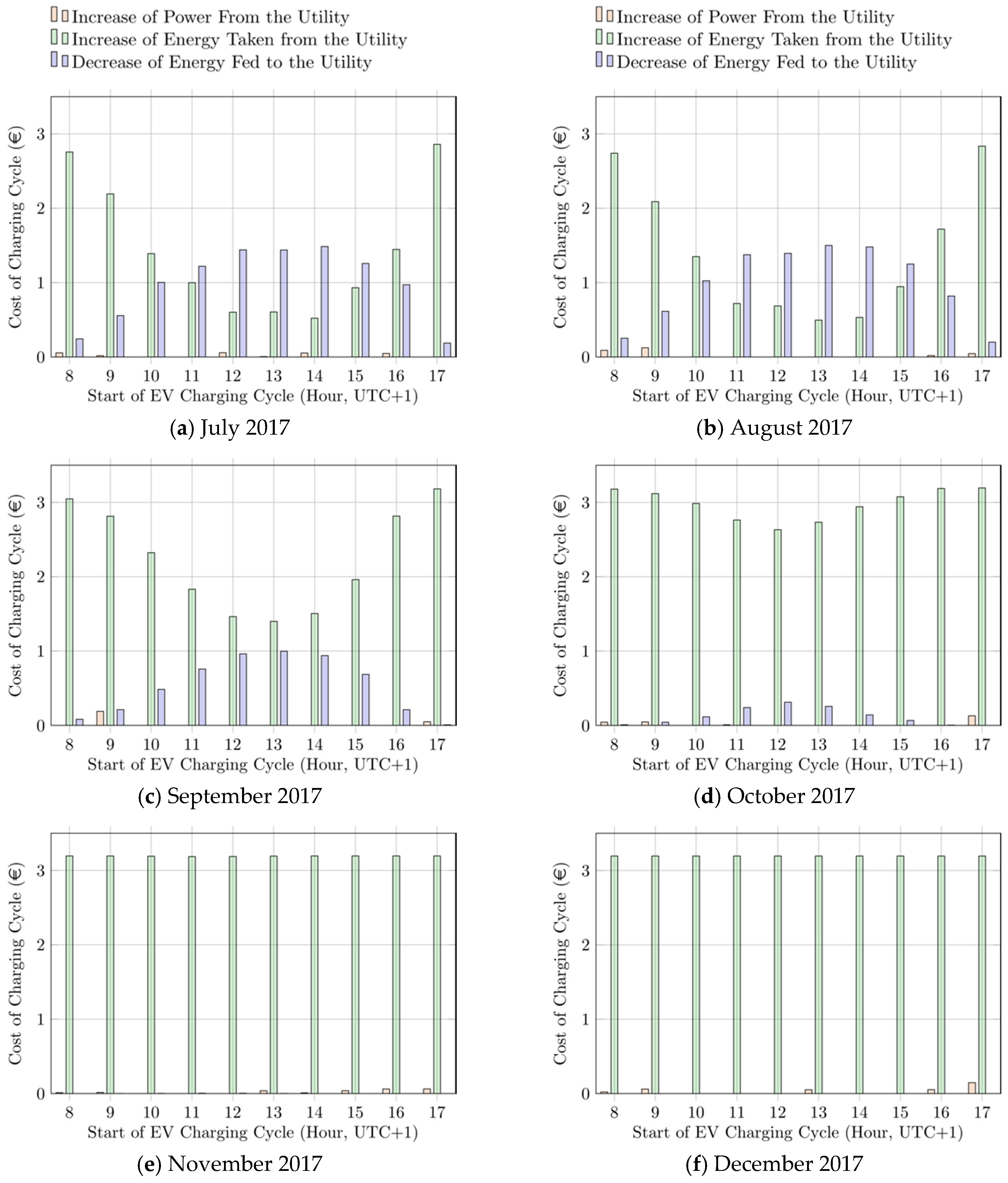
To better estimate the effect of each tariff component on the overall computed EV charging cost, in Figure 10 and Figure 11, the EV charging cost components (reported in €) from January to June 2017, and from July to December 2017 are reported, respectively. The cost components are presented for each charging cycle, depending on the time of arrival of the EV at the charging station.

As it can be noted by the analysis of the cost components, during seasons with low PV production (i.e., from October to March), the cost due to the amount of energy purchased by the grid is predominant over the other costs, thus leading to overall costs close to the applied TOU tariff. Conversely, during seasons with higher PV production (i.e., from April to September), the costs due to the loss of revenues related to the amount of energy self-consumed and not sold to the utility become more relevant, such as during late mornings and early afternoons of July and August. This clearly explains why during such periods the computed EV charging cost is noticeably lower than the considered TOU tariff. Finally, it must be noted that the effect of the demand charge cost component is almost negligible because of the low value currently applied for the rated power tariff.

5. Conclusions

The results of the simulation show that, as expected, the contribution of distributed PV generation to the charging costs of EVs strongly depend on the period of the year and on the time of connection of the EV to the EVSE during the day. At the same time, the results also show that the application of the proposed model is able to better estimate the EV charging costs with respect to the TOU energy tariffs applied by the utility. In particular, during seasons with higher PV production (i.e., from April to September), the computed EV charging cost resulted noticeably lower from the considered TOU tariff, with a highest difference of about 0.07 €/kWh. It must be noted that this value corresponds to a difference of 1.24 € per each EV charging cycle, which leads to a possible saving estimation of about 40% with respect the TOU tariff.

These results can lead to two main conclusions. First, the evaluation of the charging costs of EVs as function of the period of the year and of the time of the day must be considered to optimize the use of prosumers’ DERs. Secondly, even though it is apparent that the application of variable EV charging tariffs (i.e., compared to flat pricing schemes) could be used to promote the self-consumption of renewables, a detailed estimation of the charging costs of EVs is required to determine proper price signals that would not affect the operational costs of the system.