Robust Day-Ahead Forecasting of Household Electricity Demand and Operational Challenges


MINES ParisTech, PSL University, PERSEE—Center for Processes, Renewable Energies and Energy Systems, 06904 Sophia-Antipolis, France
*
Author to whom correspondence should be addressed.
Energies 2018, 11(12), 3503; https://doi.org/10.3390/en11123503
Submission received: 4 October 2018
/
Revised: 21 November 2018
/
Accepted: 13 December 2018
/
Published: 15 December 2018
Abstract
:In the recent years, several short-term forecasting models of household electricity demand have been proposed in the literature. This is partly due to emerging smart-grid applications, which require these kinds of forecasts to manage systems such as smart homes, prosumer aggregations, etc., and partly thanks to the availability of data from smart meters, which enable the development of such models. Since most models are academically developed, they often do not address challenges related to their implementation in a real-world environment. In the latter case, several issues arise, related to data quality and availability, which affect the operational performance and robustness of a forecasting system. In this paper, we design a hierarchical forecasting framework based on a total of 5 probabilistic models of varying complexity, after analyzing the respective performance and advantages of the models with an offline dataset. This multi-layered framework is necessary to address the various problematic situations occurring in practice and abide by the requirements for a real-world deployment. The forecasting system is deployed in a real-world case and evaluated here on data from 20 households. Field data, comprising forecasts and measurements, are analyzed for each household. A detailed comparison is drawn between the online and offline performances. Since a notable degradation is observed in the operational environment, we discuss at length the reasons for such an effect. We determine that the exact settings of the training and test periods are marginally responsible, but that the main cause is the intrinsic evolution of the demand time series, which hinders the forecasting performance. This evolution is due to unknown household characteristics that need to be monitored to provide more adaptable models.
1. Introduction
The emergence of smart grids has resulted in new business models and applications, featuring short-term forecasts of electricity demand at a local scale ranging from households to feeders. These kinds of forecasts are requested by different actors and applications: i.e., by Home Energy Management Systems to manage smart homes, and by aggregators or retailers to optimize the supply cost for a group of consumers in their portfolio. Aggregators can also offer flexibility to network operators based on their pool of individual clients. Efficiently predicting household demand is important for these actors to optimize the cost of supplying their customers and to anticipate energy purchases. Retailers can offer electricity flexibility to network operators based on their pool of individual clients. Businesses usually rely on the day-ahead electricity market—such as the EPEX or Nord Pool spots. For this reason, the focus in this paper is hourly day-ahead forecasts of household electricity demand. The development of such forecasting models has been feasible in recent years thanks to the availability of data from smart meters. In Europe, the European Parliament has enacted the roll-out of smart meters, with a landmark of 80% deployment by 2020 in most countries [1]. Individual smart meters record the electricity consumption of a household during a fixed period, e.g., one hour. Collecting such data is seen as a key factor to reach the EU energy policy goals, because it enables precise evaluation of action plans [2] and empowers consumers with detailed feedback about their electricity consumption [3].
Although a wealth of literature exists on load forecasting at regional and national scales, few studies examine load forecasting at customer level. Forecasting household demand is not straightforward. Different households have very different electricity usage profiles depending on the number of inhabitants, their lifestyle, the floor area, and other factors. Moreover, consumption in each household varies considerably from one day to the next due to house occupancy and activities, weather conditions etc.
The literature on load forecasting at local scale has grown in the last few years. The models proposed look for the most informative inputs—such as quantifying the temperature influence [4] and identifying the relevant household characteristics [5]—to make use of mature statistical methods—such as kernel density estimator [6] and copulae [7]; machine-learning techniques—such as neural networks [8] and support vector machines [9]; and original hybrid methods—such as household activity pattern modelling coupled with standard forecasting techniques [10]. A recent review of forecasting methods at the smart-meter level is proposed by Yildiz et al. [11]. This anticipation of the future electricity demand of a household is then required by other applications, such as to optimize the operation of a microgrid [12,13], or to manage smart homes through an aggregator [14]. The required forecasting horizons range from a few hours to few days ahead depending on the application. Hereafter, we consider a day-ahead horizon which is typical for applications related to electricity markets.
In most of the literature, the forecasting quality is assessed in an offline context, i.e., the forecasters work with a fixed dataset over which they have total control. In particular, the data selection is often non-detailed and follows the forecaster’s own rules, such as household choice, removal of absurd values etc. While this kind of selection is necessary to highlight the interest of the forecasting models, it does not necessarily reflect the real-life situations. In the real world, the availability of smart-meter data collection is far from perfect due to faulty meters and communication issues. Some studies [15] present efficient methods to fill in the incomplete data at the aggregated level, whereby a central agent gathers and manages the data. However, in the absence of a central agent, i.e., in a distributed context, other standalone strategies need to be employed.
The European project SENSIBLE demonstrates the use of energy storage for buildings and communities. It requires the deployment, for each household, of a day-ahead electricity demand forecasting model [16]. Since the performance of demand forecasting is known to be quite poor at the household level—state-of-the-art errors range from 5% to 60% [11]—a probabilistic output is employed to quantify the uncertainty, following a current trend in the forecasting literature [17]. In the frame of SENSIBLE, an operational load forecasting platform was set up to predict the consumption of each household at the demonstration site of the city of Évora in Portugal. The platform retrieves information from the smart meters at each household through appropriate application programming interfaces (APIs). The outputs of the forecasting models are then transmitted to other applications to be used as inputs, such as Home Energy Management Systems [18]. Hereafter, we focus on the day-ahead horizon. Specifically, our model should provide the probabilistic forecasts at 12:00 on day of the future demand expected on day D at 0:00, 1:00, ⋯, and 23:00, i.e., for horizons of 12, 13, ⋯, and 35 h. In such a use case, several features are required for the forecasting model to be implemented:
- High robustness: demand forecasts are required at all times in all situations, e.g., new house, faulty meter, etc., with reasonable performance.
- Fast computation: the model should carry out demand forecasts in a reasonable time for a potentially large number of households than can range from hundreds to thousands.
- Easy replicability: the model should be easily replicable for many household typologies and demand profiles.
- Remote control: no direct intervention is possible in situ.
- Easy interpretation: finally, among two competitive models with equivalent performance, some end-users may have preference for a model that is understandable by anyone, instead of a black-box approach.
To address these requirements, in Section 2, we introduce 5 forecasting models—and a reference model based on machine learning—at the household level. These are combined in a hierarchical framework so that they can always provide a forecast output. In Section 3, we (1) analyze the respective performance of each model with an offline dataset and (2) identify the possible situations preventing the usage of a specific forecasting model to (3) propose a hierarchical framework to design a foolproof forecasting model. After deployment in 2018 at the demonstration site, the field experience is used to evaluate the performance of the forecasting hierarchical framework. A comparison between this online performance and the offline performance is drawn and discussed in Section 4.
The key contributions of this paper lie in the proposal of a probabilistic approach for forecasting household electricity consumption. Given the operational requirement for high availability in the forecasts, a robust approach is proposed based on the operation of alternative models of varying complexity combined through a hierarchical approach. In contrast to most academic approaches in the literature, here we compare the simulation results under ideal conditions (i.e., in terms of input data availability) with field tests featuring erroneous or missing data. This provides a realistic view of the level of load predictability at local scale.
2. Case Study and Models
Firstly, we describe the offline dataset collected in bulk with the smart meters set up as part of the SENSIBLE project. Secondly, we define the selected input values that are to be fed into the forecasting models we then introduce. Finally, we present the different scores that are used to assess the forecasting performance of the models.
2.1. Offline Data Set
As part of the SENSIBLE project, smart meters are set up in a localized neighborhood in Évora, Portugal, and record the hourly electricity demand of each of the 226 households of the neighborhood. The recordings collected during the 8760 h in 2015 form the offline data set, made up of 226 individual time series. A mean demand time series is created by averaging the demand of the 226 individual households.
Following common practice, this dataset is divided into a training period to fit the models’ parameters, from 1st January to 30th September—6552 values, and a test period from 1st October to 31st December—2208 values. This separation is made to emulate real-life conditions where a model is trained and then installed for operational use. In this case, the forecasting model is trained with historical data, and then deployed at a given instant, on the 1 October 2015, to be tested over 3 months. The recordings collected during the 8760 h in 2015 form the offline dataset, made up of 226 individual time series. Advanced learning techniques exist, such as a recursive training process that regularly refines the model parameters with the most recent data, blurring the lines between the training and test periods [19]. We do not consider such techniques here since they require high maintenance.
2.2. Input of the Forecasting Models
An efficient forecasting model makes use of informative inputs to produce relevant forecasts. Based on the electricity demand forecasting literature and to keep a small input set, we select only two kinds of information: historical data of demand measurements, and local outside temperature.
2.2.1. Historical Demand Measurements
Recent demand measurements, i.e., lagged values of the time series, constitute precious information when forecasting future demand [20]. Selecting the most informative lagged values is tricky and is ideally made for each household separately. A common practice is to analyze the partial auto-correlation function. This function quantifies how much each lagged value is correlated with the current value independently of the values in between, e.g., how much is correlated with after removing the correlation effect between and [21]. However, selecting automatically how many lagged values and which ones for each household is often cumbersome, and hinders the replicability of the model. For instance, the number of relevant lags change with household, and consequently, they modify the complexity of the models.
Here we consider that the primary interest is to develop a model that is easily replicable for a (very) large number of households that range from hundreds to thousands. We therefore opt to keep only two lagged values that proved efficient on average:
- The measurement made 24 h before the instant to forecast , which is highly informative due to the strong daily seasonality.
- When the forecasting horizon is superior to 24 h, the measurement made 48 hours before is used as a direct surrogate.
- The median demand made on the previous week , which reflects the recent behavior.
While these two historical inputs are related, both are insightful: the value observed the previous day is volatile and depends on the specific inhabitant’s activity on this particular day, the median value of the previous week conveys the recent habits in a smoother manner.
2.2.2. Outside Temperature
The impact of the local outside temperature on electricity demand is generally recognized [22]. For forecasting purposes, we retrieve the local temperature predictions made on the previous day from a Numerical Weather Prediction (NWP) model. In this case, study, we consider NWPs provided by the European Centre for Medium-Range Weather Forecasts (ECMWF) [23]. For the offline dataset, and to mimic the real application, we retrieve the deterministic forecasts made at 12:00 for the next day, i.e., with forecasting horizons of h. In fact, ECMWF provides only one forecast value every 3 h, and, hence, the gap hours are filled with a linear interpolation. Therefore, the temperature forecasts produced at 12:00 on 31 December 2014, 1 January 2015, ⋯, 30 December 2015 are collated in a time series, noted , comprising the 8760 hourly temperature values in the neighborhood in 2015. For the online usage, the NWPs are directly retrieved at the household level through an API. Although some studies show that lagged values of the temperature slightly improve the electricity demand forecasting performance, we select only one single value to keep the model simple and interpretable [24].
2.3. Forecasting Models
To provide a day-ahead probabilistic forecast of the electricity consumption of a household at all times, we propose a total of 5 alternative models of increasing complexity: 2 “climatology” models, 2 temperature-dependent models, and 1 additive model. These models are meant to be used in a hierarchical manner to always provide the most accurate forecast depending on the situation. Additionally, a reference model based on machine learning is introduced as a benchmark. The models’ parameters are fitted to the data from the training period, to keep out-of-sample the data from the test period [25]. Each model is probabilistic and produces a set of forecasts for instant t at quantile levels . The median probabilistic forecast at level is used as the point/deterministic forecast.
2.3.1. Climatology Models
We create a “climatology” type of model for each one of the 226 households. This kind of model was early introduced in the weather community [26] and consists in computing quantile forecasts based on all the historical observations unconditionally. In our case, all the demand measurements of the training period made on a given day of the week and hour of the day are used to compute fixed quantile values for this hour and day, independently of the recent demand values or the weather conditions. This method means that the forecasts for every Monday are always the same, be it in August or in December.
The 1512 () values computed from the training period provide a quantile forecast of the demand for any future instant t, noted .
This climatology model is then referred to as for household . Additionally, we create an average climatology model, referred to as , based on the mean demand time series.
2.3.2. Temperature-Dependent Models
Since the temperature time series is retrieved from a different source than the smart-meter measurements, the presence of this input is expected to have a different reliability. Usually, given a good internet connection, the availability of NWPs is high. They are also provided several times per day and even if once they are not available one can use forecasts from previous runs of the NWP model. For this reason, it is useful to design a forecasting model relying solely on this information. Quantile smoothing spline functions are fitted by optimizing with the quantile score as a loss function. The fit is done with function rqss implemented in the R package quantreg [27]. Since the temperature has a different impact on demand depending on the hour of the day, a total of functions are fitted, for , so that
is the quantile forecast of the demand at level , where the instant t to be forecast is associated with the hour h of the current day. In practice, the function is not fitted to the actual demand , but rather to the residual errors after shifting the demand value by the median climatology forecasts. Our experiments, not reported here, show that proceeding as such slightly refines the spline fitting process.
This temperature-dependent model is then referred to as for household . An average temperature-dependent model, using the mean demand time series, is also fitted, and noted .
2.3.3. Additive Model
Three independent quantile smoothing spline functions are fitted to the data of the training period to reflect the effects of three inputs: the demand measured 24 h before, the median demand during the 7 previous days, and the temperature forecast. The fit is done with function rqss implemented in the R package quantreg [27]. An additive structure is selected to simplify the fitting process, and a fit is done for each hour of the day h, so that
is the quantile forecast of the residual error at level , where the instant t to be forecast is associated with the hour h of the current day. As with for the temperature-dependent model, the fitting is made on the residual errors rather than the actual demand. The fitting process for the 6552 points of the training period is fast, i.e., less than 5 seconds on an average 2013 laptop. In the literature, this kind of additive framework proves efficient when forecasting electricity demand [20].
This additive model is then referred to as for household . No average model is created because it would involve gathering individual smart-meter data in real time to compute the mean demand time series. Such gathering is strongly invasive of privacy and thus to be avoided [28]. Advanced methods to protect user privacy exist, such as employing a consensus framework [29] but are not considered in this study.
2.3.4. Reference Model Based on Machine Learning
Additionally, we train a gradient boosting model that makes use of the same inputs as the additive model, i.e., the demand measured 24 h before, the median demand value during the 7 previous days, the temperature forecast, and the hour of the day. A total of 9 versions are computed for quantile levels . The meta-parameters of the gradient boosting model are adjusted in such a way that the computation time for the training phase is approximately the same as for the additive model, i.e., about 5 s. This gradient boosting model is then referred to as for household . This machine-learning model is used as a benchmark due to its established performance [30]. Note that this black-box model cannot be used in the demonstration project due to its somewhat obscure behavior.
2.4. Forecasting Performance Scores
To assess the performance of a forecasting model, we compare the forecast values with the observations during a test period, i.e., for . Considering a point forecast, we calculate the Normalized Mean Average Error (NMAE)
where is the point forecast for instant t, and its corresponding observation. Considering a probabilistic forecast, the aim is to calculate the reliability (Rel) between two successive quantile levels
for , where is the Heaviside function, and is the forecast quantile at level . To ensure that the forecast distribution is reliable, or calibrated, the reliability for interval k must be close to the theoretical frequency . This frequency is never exactly observed due to natural statistical fluctuation, so Candille and Talagrand propose a reliability ratio that quantifies how well-calibrated the forecast distribution is, see [31] (Section 3). In addition to the reliability, we compute the Normalized Quantile Score (NQS) to check the accuracy of the probabilistic forecasts. Specifically,
The NQS is negatively oriented: a lower value indicates a better performance at quantile level . Note that .
3. Hierarchical Forecasting Framework
We first select a subset of 20 households with high-quality smart-meter data to assess the performance of each forecasting model. Then, we identify the problematic situations occurring in practice, before finally designing a hierarchical forecasting framework combining the models based on their respective performance and robustness to problematic situations.
3.1. Offline Forecasting Performance of a Subset of Households
For each household, we have 6 alternative day-ahead forecasting models, , , , , , and .
Based on their respective level of complexity and the forecasting literature, we expect similar performance from and , and that both will outperform , then , then , and then . We wish to assess their respective performance during the test period going from 1 October to 31 December 2015. To perform this evaluation, we select a subset of households based on two criteria:
- The availability of the smart-meter data of the household should be almost perfect. We only retain households whose demand data are available at least 95% of the time in both the training and the test periods.
- There should be no abrupt change in demand patterns between the training and the test periods. This is assessed by examining the climatology probabilistic forecasts computed during the training period. With such a model, the reliability of the forecast should be fairly correct during the test period when no abrupt changes occur. Therefore, we check that the reliability ratio defined by Candille and Talagrand, see Section 2.4, is close to the ideal ratio of 1. Somewhat arbitrarily, we choose that a household passes this reliability test when the ratio is below 20.
A subset of only 20 out of the 226 households fulfill the two criteria, later denoted subset . In fact, most of the 226 households exhibit abrupt changes in their demand patterns that are quite difficult to anticipate, and that do not reflect the intrinsic performance of the forecasting model.
For the 20 households in the subset , we compute the Reliability and the Normalized Quantile Score, see Section 2.4, for the 6 models introduced. The average results are shown in Figure 1, and in Table 1.
When examining the reliability ratio, we observe that the specific models are reasonably calibrated but that the average models are not. The whole forecast distribution of the latter either overestimates or underestimates the demand. Consequently, providing point forecasts of the demand of an unknown household is reasonably efficient—NMAE around 31.1%—but providing average probabilistic forecasts makes no sense and requires specific measurements of the corresponding household.
The quantile score curves, visible on the right panel in Figure 1, depict the performance at different quantile levels, i.e., for different parts of the forecast distribution. The values of the NMAE scores are readable at quantile level 50% and indicate which forecasting model is better to provide point forecasts.
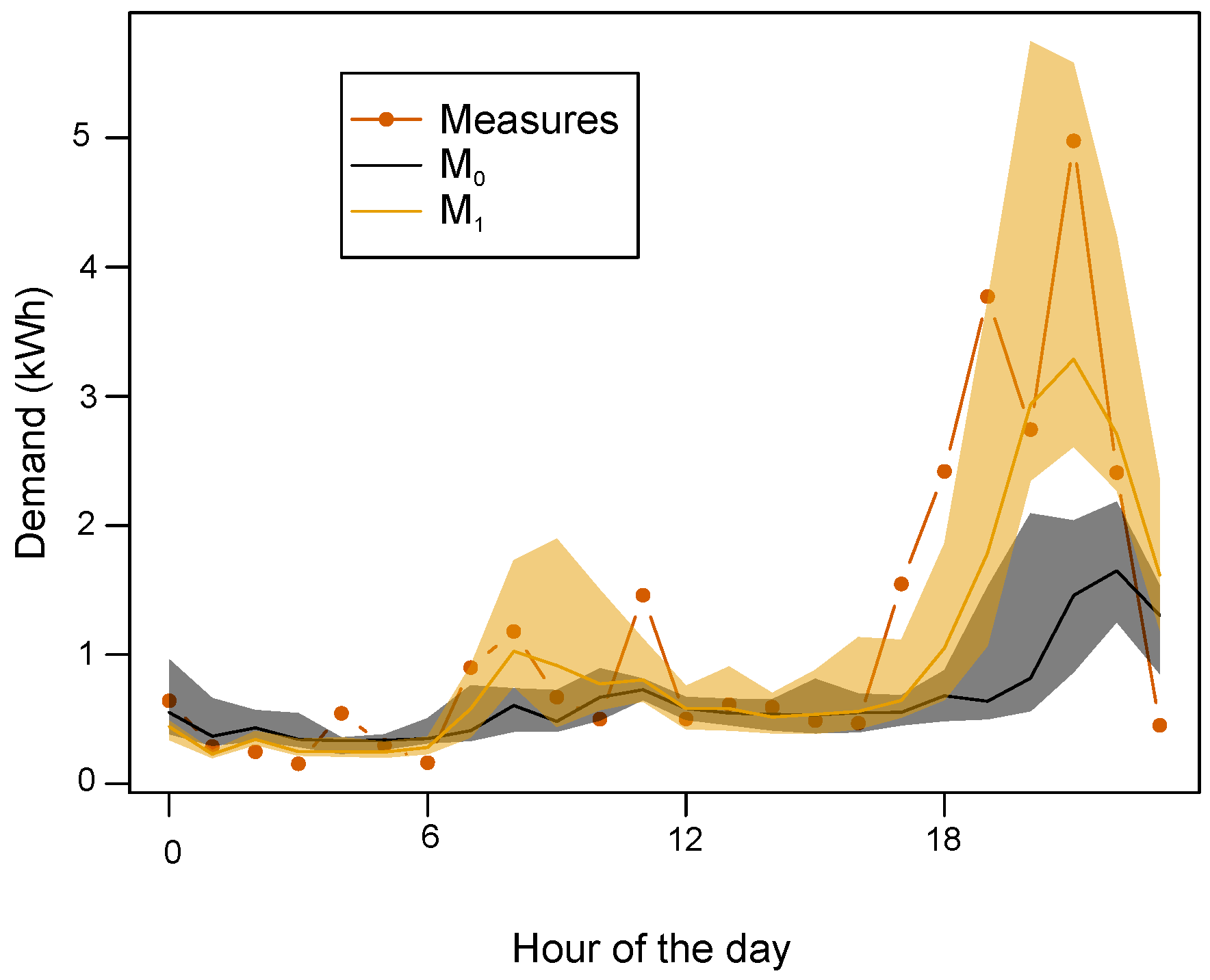
We see that the performance of each model is ordered as expected, with a top performance of 27.2% for . The hypothesis that all 5 models have similar performance is rejected according to the Friedman statistical test (p-value of ) [32]. Additionally, we note that the most efficient proposed model M has similar performance to the reference model : the nonparametric Wilcoxon test does not reject the null hypothesis claiming similar performance (p-value of 0.54) [33]. On average, the models specifically trained for households decrease the errors by around 10% in comparison with the average models. This relative improvement is intensified when considering the distribution tails. The curves crossings between the models suggest that forecasters should use the additive model for lower quantile levels (10–60%) and then switch to the specific climatology model for higher levels. This observation highlights that it is, perhaps surprisingly, more efficient to carry out conservative forecasts for the upper part of the forecast distribution. However, this conclusion should be adapted depending on the household considered. For instance, for about one third of the households, the models with a temperature input, i.e., M and M, clearly outperform the climatology M at all levels. Identifying these households that benefit from the temperature input is quite straightforward: they are equipped with heating or cooling electrical devices, i.e., they have clear thermal sensitivity [34]. This sensitivity is measured by retrieving the correlation between the electricity demand and the outside temperature. Thermal sensitivity is defined as the squared correlation and so a high (resp. low) sensitivity depicts a strong (resp. weak) demand–temperature correlation. The households with high sensitivity show a clear increase in electricity demand when it is cold outside. In these cases, the forecasts are more accurate as illustrated in Figure 2, where the evening demand is well anticipated by the temperature-dependent model M (orange) since it is a cold day, but not by the climatology model M (black).
3.2. Problematic Situations
Although the additive model provides the best performance, it is also the least robust model and several problematic situations occasionally prevent its usage. This is often the case for similar type of models based on time-series approach. The following situations are identified to be problematic when forecasting the demand of household :
- No data in the training period. There is no way to create the specific models , , and .
- No temperature forecast. Models making use of the temperature , , and are missing an input and cannot properly carry out a forecast.
- No recent measurements. Input values or are then unavailable, meaning that cannot operate.
- Unknown situation. A drawback of the smoothing splines is that extrapolation is known to perform poorly, affecting the activation of A, M, and M. For instance, if recently observed demand values have never been this low in the training set, it is better to refrain from using the additive model .
3.3. Hierarchical Framework
3.3.1. Flowchart
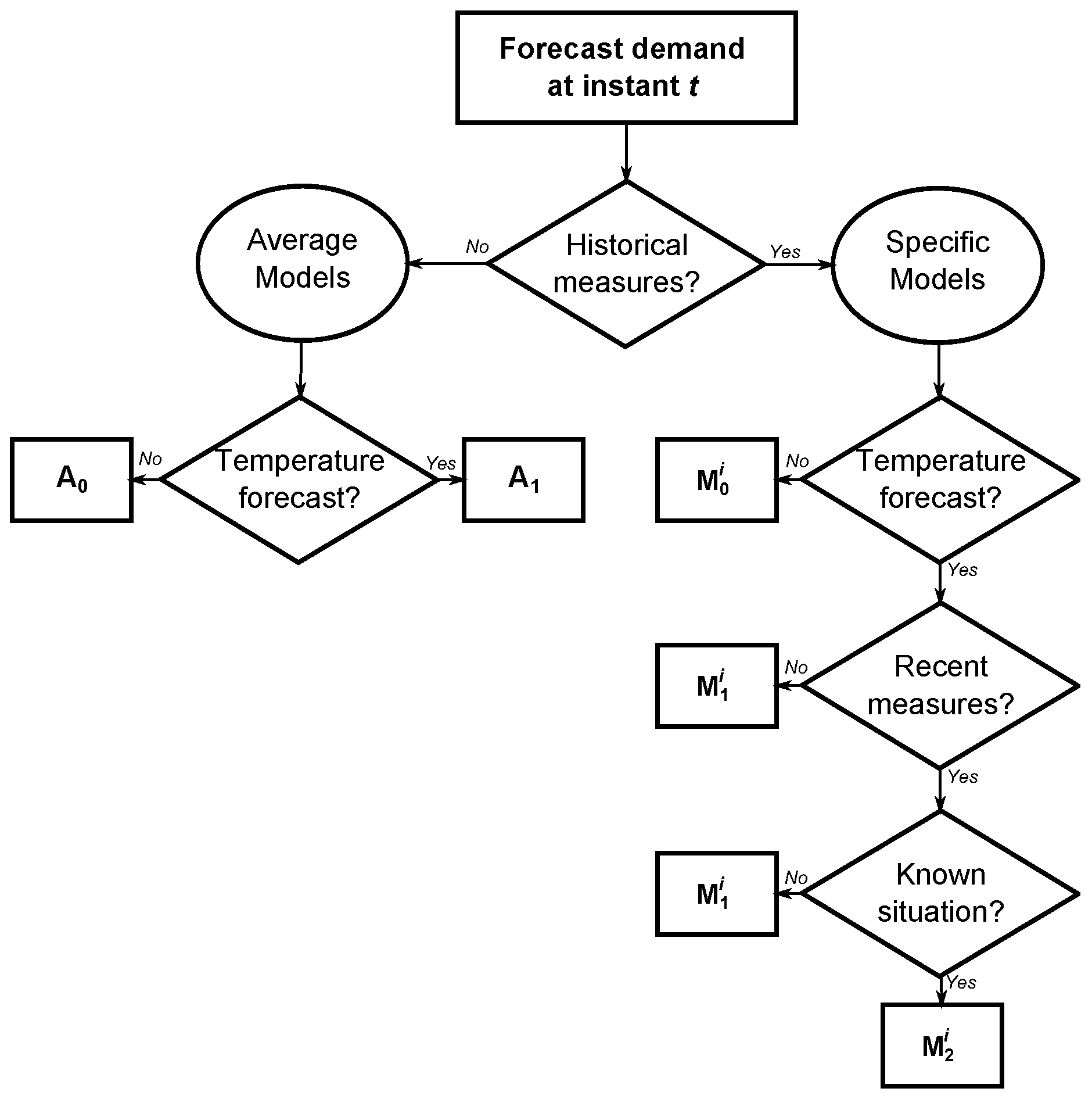
The respective performance of each model coupled with the identification of problematic situations enable us to design a forecast hierarchical framework represented in Figure 3. In the implementation, when producing a forecast for instant t for a household i, we successively check:
- Are there historical measures specific to this household?
- Is there a temperature forecast available?
- Are the recent measures and available?
- Is the future situation known, i.e., do the inputs values extrapolate from the ones that occurred during the training period?
3.3.2. Performance
We implement the hierarchical framework for each of the 226 households in the neighborhood. The flowchart detailing the model usage according to the situation allows us to always provide day-ahead probabilistic forecasts for each hour of the day in the test period—from 1 October to 31 December 2015. We assess the performance by comparing these forecasts to the available data. Since some households have missing demand measurements, the length of the test period is not the same for all the households. For instance, one household has no measurement at all in December and so the performance is estimated with a test subperiod going from 1st October to 30 November.
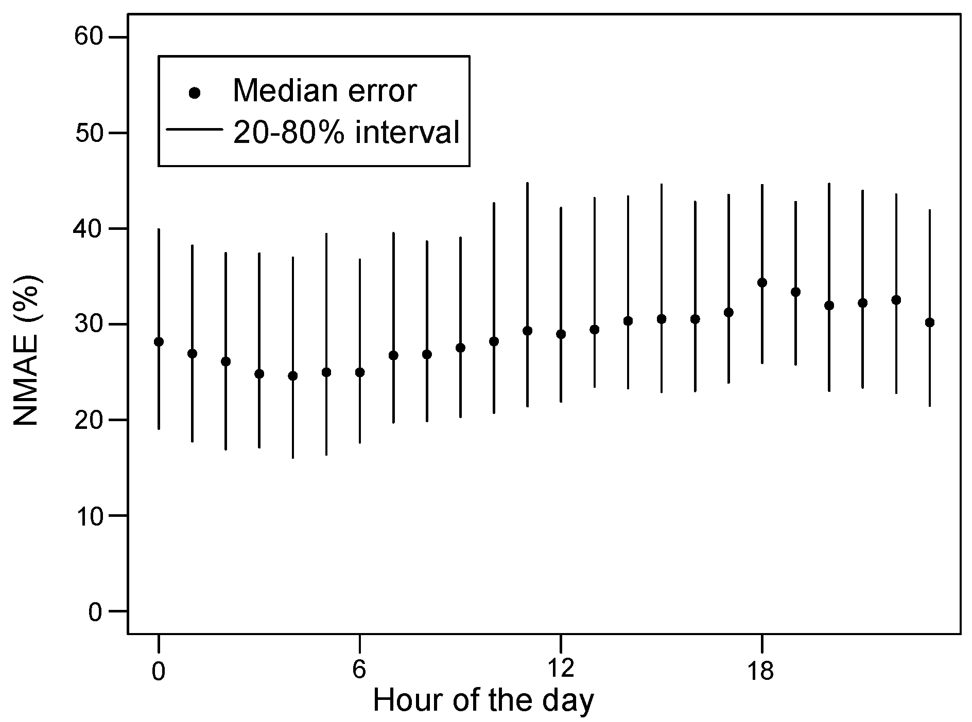
Figure 4 depicts the NMAE observed for each hour of the day among all the 226 households. The points show the median NMAE, and the segments show the variation 20–80% among households. The errors follow the same trend as the actual demand values: lower in the nighttime, and higher in the evening. However, the fluctuation throughout the day is minor. Since all the forecasts are carried out at 12:00 on the previous day, forecasts for a specific hour of the day represents a specific horizon. It means that errors at 0:00 correspond to a forecasting horizon of 12 hours, errors at 1:00 correspond to a forecasting horizon of 13 h, and so on.
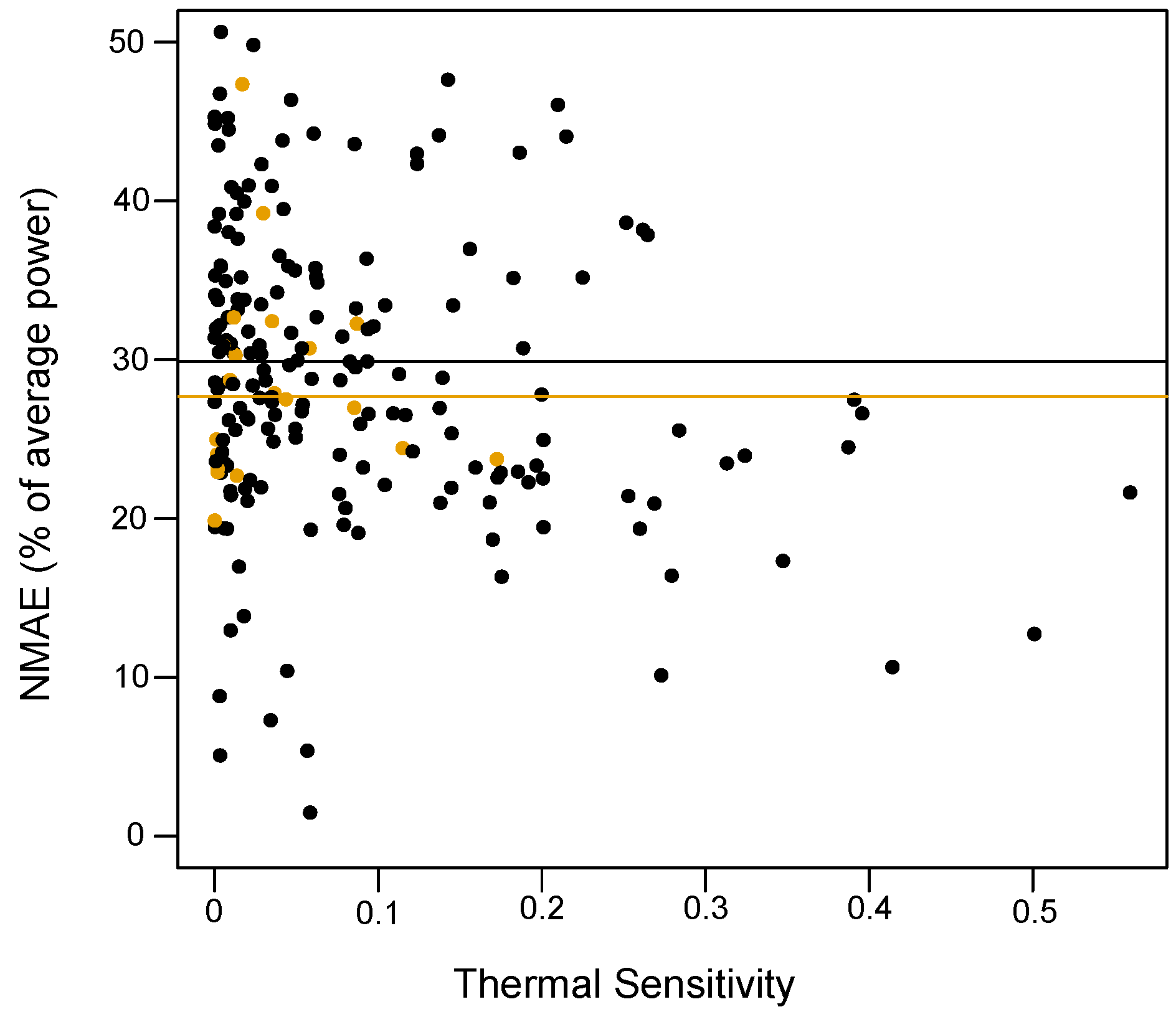
We then represent the NMAE, averaged over the 24 h, as a function of the thermal sensitivity in Figure 5.
The households in the subset are represented by the orange dots, and the rest by black dots. We can see that the model performs slightly better on the subset : the median NMAE decreases from 29.9% to 27.7%. The graph also logically shows that households with greater thermal sensitivity are easier to forecast. Additionally, we can see that performances greatly vary between households with similar sensitivity: errors range from 2% to 51% for low sensitivity (below 0.1). This is due to the unknown behaviors of the householders and other cultural factors, e.g., the number of appliances in the house. It highlights that anticipating a forecasting performance for a different use case should be done with caution.
4. Offline and Online Performances
We first draw a household-by-household comparison of the offline and online forecasting performances. Then, we discuss and quantify in detail the factors that cause a noticeable performance degradation with precise test cases.
4.1. Performance Comparison
The hierarchical forecasting framework is implemented at the Évora demonstration site. The forecasts produced and smart-meter measurements are retrieved, providing a recent online dataset. This dataset is made up of two parts: a training period going from July to December 2017, and a test period from April to August 2018.
We first analyze the frequency with which each one of the 5 models that compose the framework, depicted in the flowchart in Figure 3, are activated as a function of the available data. The results are given in Table 2. It is noted that, at each instant, a single model produces the final forecast, according to the situation. The most efficient model M is activated in about three quarters of the cases. We observe similar model activation frequencies in the online and offline cases.
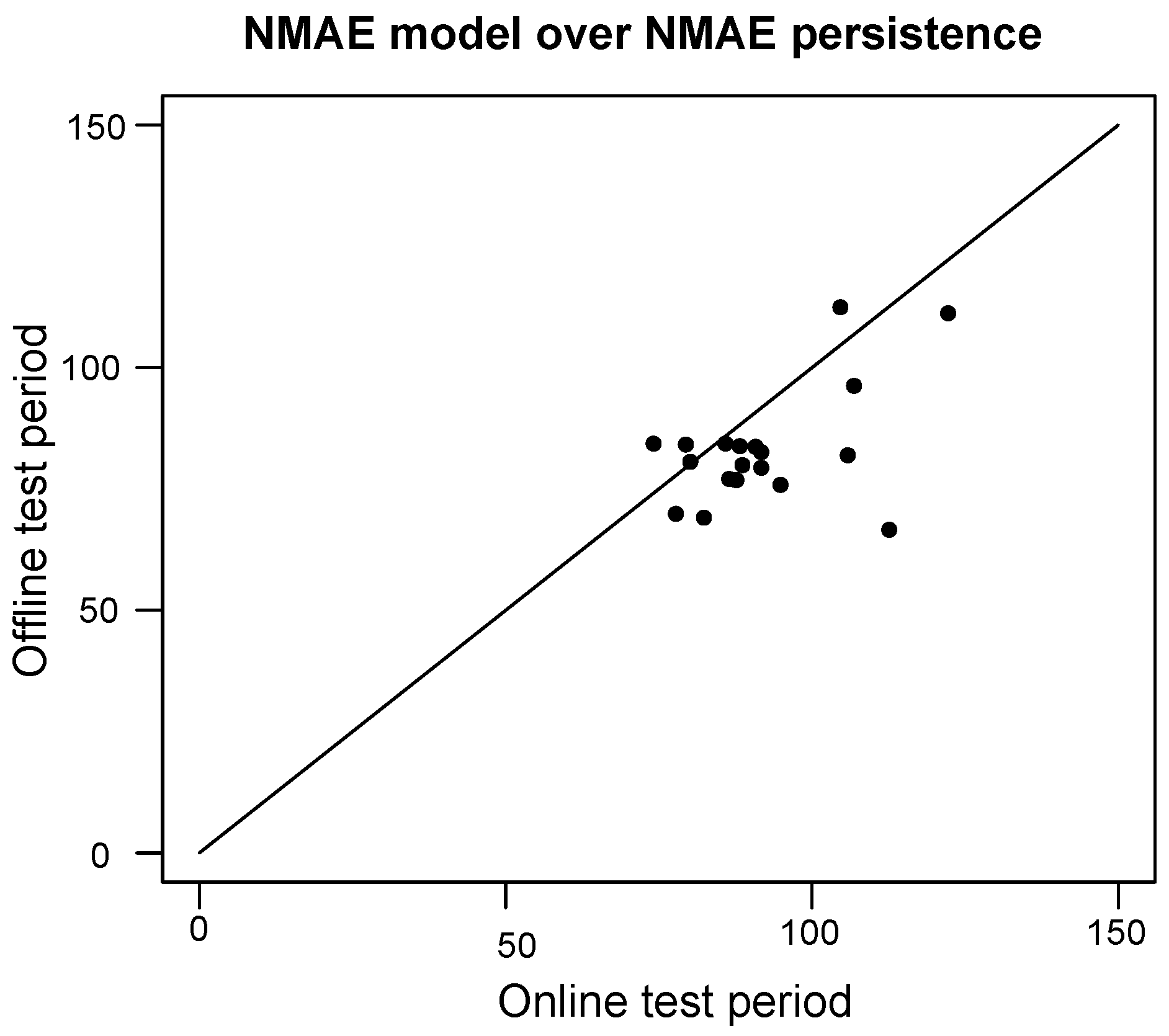
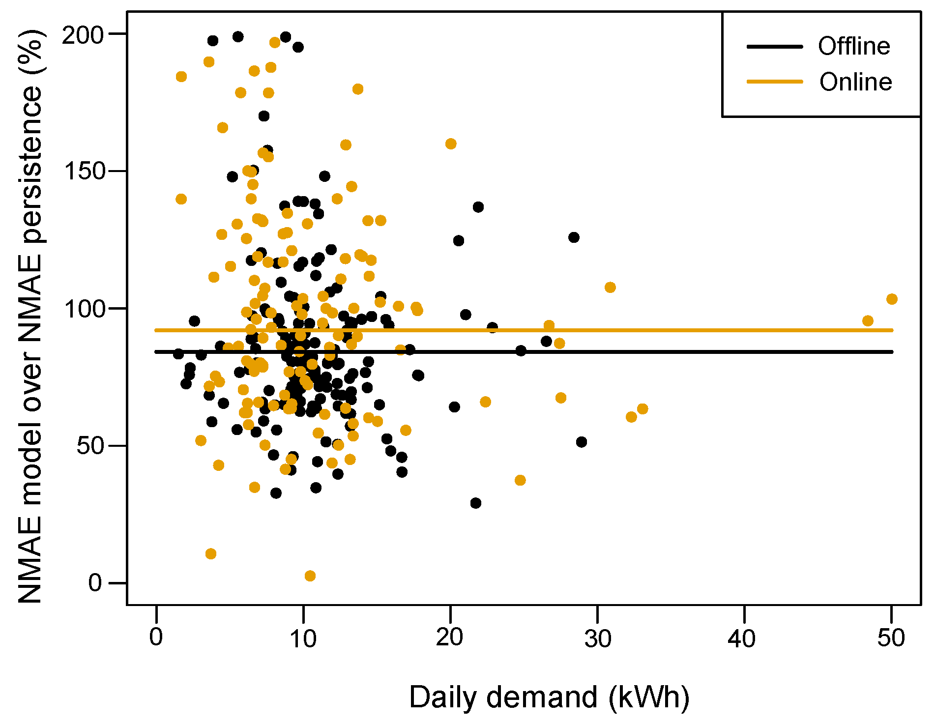
The online data is collected from the 20 households of the subset introduced in Section 3.1. Figure 6 compares the performance of these 20 households obtained during online test period—1 April to 31 August 2018—and during the offline test period—1 October to 31 December 2015. We compare the NMAE obtained during the two periods. with our forecasting framework and divide this error by the NMAE obtained with a 1-day persistence model. Note that the normalization in the NMAE score comes from the mean value observed from the sets studied, and so the normalization value evolves between the offline and online test sets. For most households, the errors made by our model is lower than the persistence errors (average of 0.90 offline and 0.97 online). Furthermore, for 17 out of 20 households, the individual NMAE obtained offline is lower than online, meaning that the model performance has decreased between the two test cases. We also provide in Figure 7 the NMAE computed over a single day. Each point, in black for the offline case and in orange for the online test, represents the ratio between the NMAE of our forecasting framework and the NMAE of the persistence model (y-axis). The daily demand of the day (in kWh) is represented on the x-axis. We see that the daily performance is more volatile when the demand of the day is low than when this demand is important. In fact, this performance volatility is due to the persistence forecasts performance that also widely range for low-demand day: performance is either very good (when the previous day is also a low-demand day) or very poor (when the previous day is not a low-demand day). The improvement over persistence is clearer for high-demand days in online and offline cases.
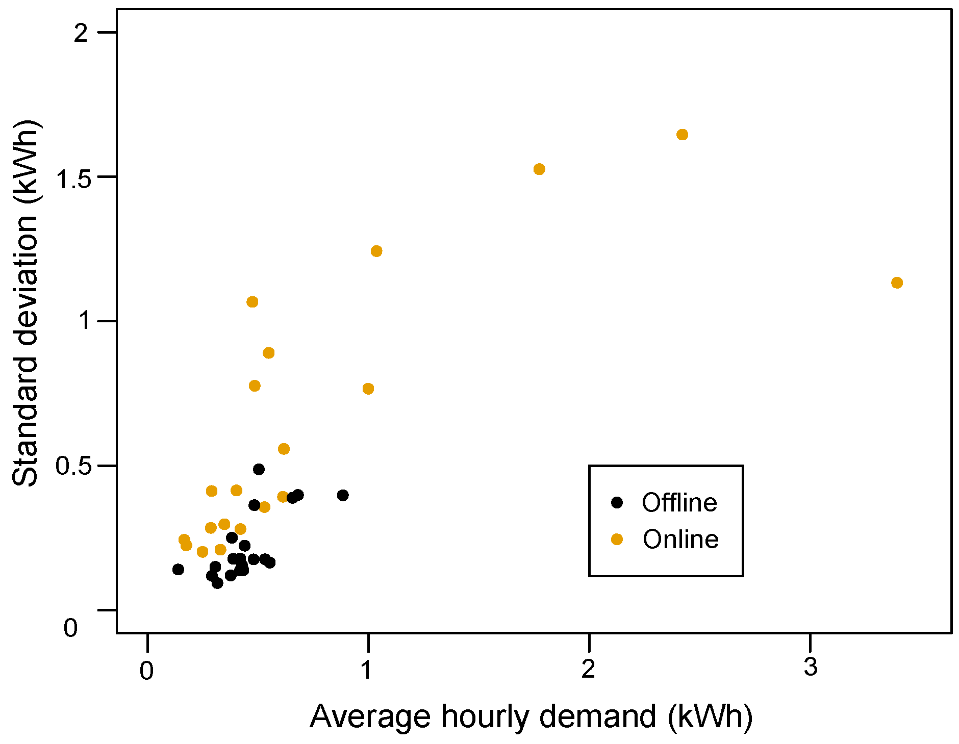
On average, the online performance is worse than the offline performance. In absolute values, the average NMAE goes from 34.8% on the offline test to 58.5% on the online test. This comes from the demand characteristics that are quite different between two cases. Figure 8 provides an indicative illustration. For the same set of households in the two cases, one point represents the average hourly electricity demand of the household (x-axis) and its standard deviation (y-axis). Both the mean and deviation largely increase between the two cases. This evolution directly influences the forecasting performance since it denotes the usage of more appliances, hence more demand volatility and forecasting complexity.
4.2. Discussion
We investigate the possible reasons for the performance degradation between the offline and online tests: the evolution of the demand time series, the availability rate in the test period, the duration and recency of the training period, the position during the year of the test period. The subsequent tests are made using our offline 2015 dataset with the subset of 20 households to quantify the possible performance degradation.
4.2.1. Evolution of the Demand
Since there is a considerable time gap between the offline test, in 2015, and the online test, in 2018, the behaviors of the householders living in the 20 households have evolved: new people, new appliances, new habits, etc. This evolution is reflected in the electricity demand patterns which modify the intrinsic complexity of the forecasting task. Defining this complexity is not straightforward: we examine the performance of a 1-day persistence model—by which we use the demand measured on the current day to provide point forecasts for the next day. We observe that this persistence model has an average NMAE of 45% from April to August 2015, and this error increases to 69% from April to August 2018. This means that forecasting the 2018 time series is roughly 50% more difficult than forecasting the 2015 time series.
4.2.2. Availability Rate in the Test Period
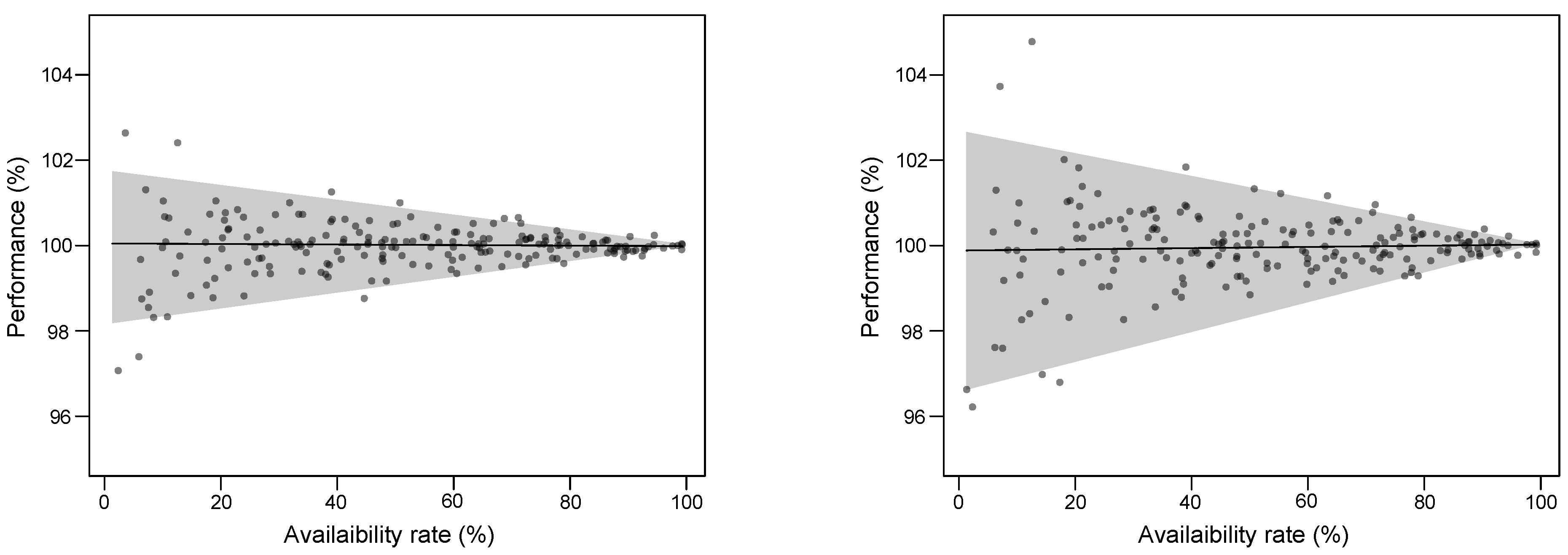
For each one of the 20 households in the subset, we randomly discard a certain amount of available measurements in the test set, obtaining an availability rate between 0 and 1. This mimics the case when a specific hourly observation is missing, and so the forecast cannot be compared to the actual observation. We compute the forecasting performance of M with the NMAE and indices on the available subperiod. In Figure 9, we represent the performance fluctuation (in %) regarding the availability rate. Logically, we see that the average performance is constant, i.e., at a reference level of 100%, whatever the availability rate. However, note that the missing values introduce variability in the performance evaluation. This variability logically increases when the availability rate decreases. It goes up to 2% when examining the NMAE. This effect is emphasized for the distribution tails, as seen on the going up to 4 % for low rates, that are more difficult to estimate accurately.
We conclude that missing values in a test set induces limited performance fluctuation. However, the missing values here are assumed to be uniformly spread throughout the period, which is the case in the actual online dataset retrieved. Another use case may result in different missing value distribution, e.g., when a smart meter is disconnected during a contiguous period of time.
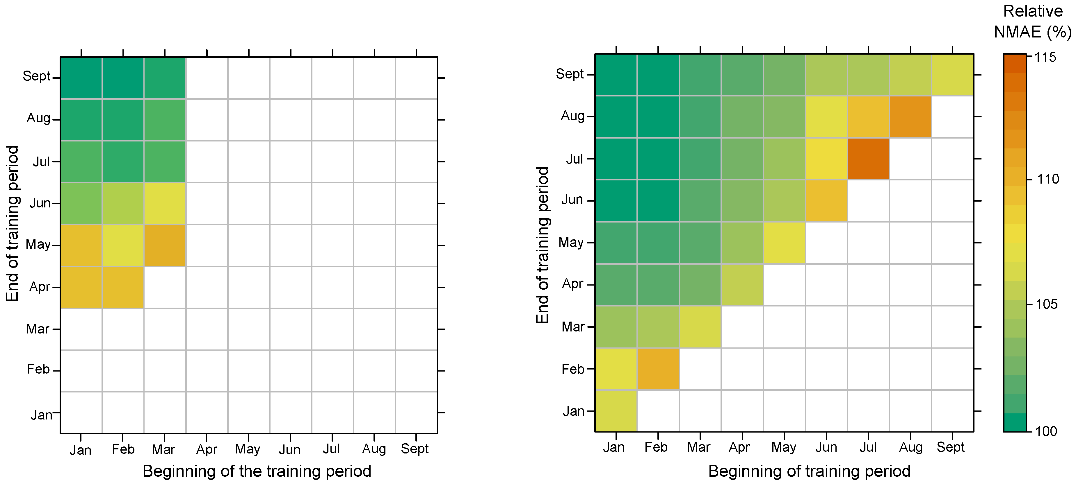
4.2.3. Training Period Position
For each of the 20 households in the subset, we train the forecasting models M and G at quantile level 50% with different training periods. Figure 10 represents the average NMAE achieved on the test period, fixed from 1 October to 31 December 2015, relatively to the minimal NMAE obtained with the longest training period going from January to September. The beginning of the training period is selected on the x-axis, and the end is selected on the y-axis. The left panel represents the performance with the M model while the right panel represents the performance with the G. Since the additive model M is not designed for extrapolation, the training period necessarily should include the first months of the year, to observe similar temperature as during the test period, to produce forecasts. It means that only a limited range of training periods could be evaluated. On the other hand, the machine-learning model G is designed for such extrapolation, so we can extend the performance on more diverse training periods. While both models produce the same performance when using the 9 months (January to September) as training sets, we see that G does a better job with reduced periods. We logically see that reducing the duration of the period damage the performance of both models. We see that the degradation can be up to 10% for M when the period lasts only 3 months (February to April) with a time gap between training and test, instead of 9 months (January to September).
We conclude that training with the all the data, and using as recent data as possible, is the best way to grasp the various recent demand patterns. Furthermore, we stress the importance of using data collected during similar situations to those to be forecast, especially regarding the temperature. For instance, to efficiently forecast summer 2018 ideally means training the model with data collected in summer 2017.
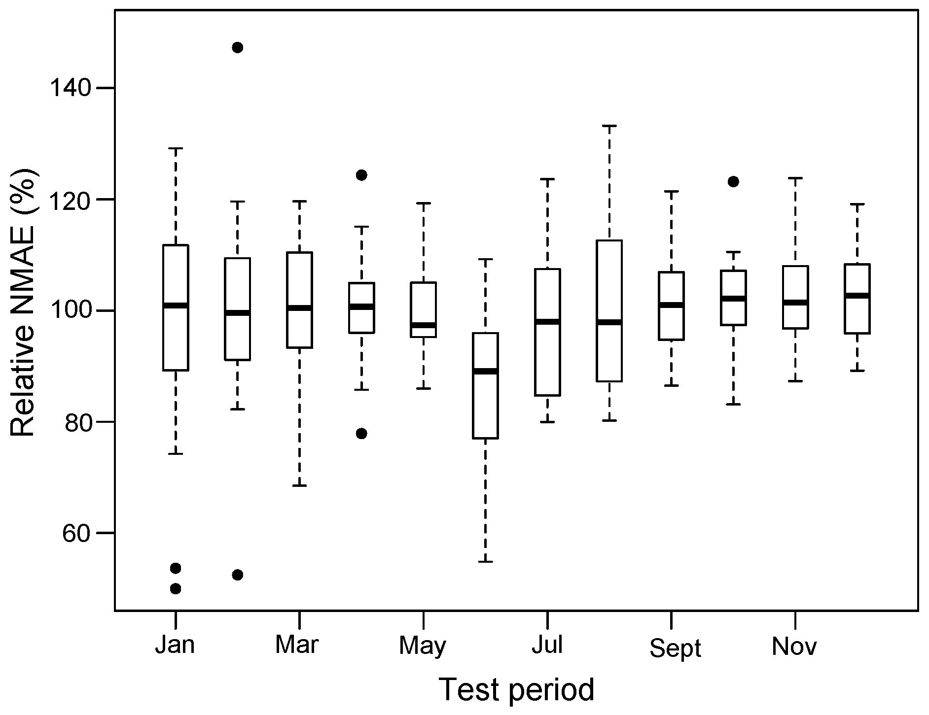
4.2.4. Test Period Position
The test period’s position in the year impacts the performance. Figure 11 represents the forecasting performance with model M obtained using, in turn, each month of the year 2015 as the test period, using the remainder as the training period. This framework implies that, while the test period is always out-of-sample, it is surrounded by the training period, which prevents any major deviation, possible in a real case. For each household in the subset, the NMAE obtained for each month of the year is divided by the average over the whole year, to obtain a relative NMAE. The boxplot representation indicates the variation in the subset. We can see that, on average, the summer period, i.e., June to August, produces a slightly better performance than the other months, with a NMAE decrease of around 5%.
4.3. Summary
As a reminder: (1) the offline training period goes from 1 January to 30 September 2015, the offline test period from 1 October to 31 December 2015, and the offline NMAE is 34.8%; (2) the online training period goes from 1 July to 31 December 2017, the online test period from 1 April to 31 August 2018, and the offline NMAE is 58.5%.
We identify that the main cause of this 68% relative performance degradation is due to the intrinsic evolution of the time series. Thanks to a simple persistence forecasting model, we assess that the demand time series in the online case are roughly 50% more difficult to forecast than those of the offline case. To a great extent, we remove this intrinsic time-series evolution by analyzing the performance improvement of the forecasting framework over the persistence model. On average, we have seen that the NMAE is reduced to 90% of the persistence NMAE in the offline dataset, but only 97% in the online dataset. This remaining relative performance discrepancy of 8% is due to the mismatch of the training and test period positions in the online case. In fact, the models are trained with fall data, but tested with spring data, which causes a relative degradation of around 15%. This effect is counterbalanced by around 5% due to the position of the test period, since the spring period (online case) is easier to predict than the fall period (offline case).
5. Conclusions
We present 5 probabilistic forecasting models that employ small input sets—day of the week, hour of the day, recent smart-meter data, temperature prediction—to produce day-ahead forecasts of electricity demand at the household level. We compare the performance of the models on an offline dataset collected at a demonstration site in a Portuguese neighborhood. We observe that the more flexible, and thus more complex, model logically results in better overall performance, similar to that of a machine-learning benchmark.
However, many problematic situations arise and prevent the usage of this flexible model in real time. We therefore propose a hierarchical forecasting framework, combining the 5 models introduced, that addresses the following requirements: high robustness, fast computation, easy replicability, remote control, and easy interpretation. These requirements are essential for deployment of a forecasting model for a large number of households in real-world applications. After deployment in 2018, in the demonstrator in the frame of SENSIBLE project, the feedback data collected at the demonstration site are analyzed to provide an online forecasting performance. A household-by-household comparison with the performance assessed using an offline dataset shows a considerable relative degradation. We quantify the possible reasons for this degradation. Although it is due, in part, to the mismatch between the online training and test periods, the main cause is the evolution of the demand. From the distance in time between the initial offline testing of the model and its implementation for real operation, we observed an evolution of the characteristics of the physical process itself. The complexity of the demand pattern has greatly increased, meaning that the forecasting task is found to be about 50% intrinsically more complex during the online test. This observation highlights the fact that assessing forecasting performance at the household level is challenging. While forecasting performance was observed to vary greatly between two households, even when located in the same neighborhood, our experimental feedback shows that this performance also significantly evolves with time. This evolution is caused by unknown abrupt characteristics changes in the household, such as new people, additional appliances, changing habits of the householders, etc.
This raises the question of the adaptability of forecasting models at the household scale. We recommend incorporating the most recent data into a training period, to which the forecasting models are regularly fitted. The regularity of this training process can be quite coarse, e.g., every month, since most recent demand patterns are only slight deviations of older ones. Such a framework still implies a degree of model maintenance, such as reviewing the validity of the most recent smart-meter data recorded and starting the training process. A more intricate issue is caused by occasional abrupt changes in demand patterns. These changes are difficult to observe solely from the electricity demand time series. We advise using external input information about such changes, e.g., moving-in of new householders, to discard obsolete data and train using only smart-meter data recorded after the changes.
Author Contributions
Formal analysis, A.G. and R.G.; Software, A.G. and A.B.; Supervision and research methodology, G.K.; Writing—original draft, A.G.; Writing—review & editing, R.G. and G.K.
Funding
This research was funded by the European Union under the Horizon 2020 Framework Programme grand agreement No. 645963 as part of the research and innovation project SENSIBLE (Storage ENabled SustaInable energy for BuiLdings and communitiEs—www.projectsensible.eu)
Acknowledgments
The authors would like to thank ECMWF, the European Centre for Medium Range Weather Forecasts, for the provision of Numerical Weather Predictions, the industrial partners of SENSIBLE project for the provision of the measurements used in this work, as well as the three anonymous reviewers who provided valuable remarks improving the quality of the paper.
Conflicts of Interest
The authors declare no conflict of interest. The founding sponsors had no role in the design of the study; in the collection, analyses, or interpretation of data; in the writing of the manuscript, and in the decision to publish the results.
References
- European Parliament. Directive 2009/72/EC concerning common rules for the internal market in electricity. Off. J. Eur. Union 2009, 4, 29–67. [Google Scholar]
- Armel, K.C.; Gupta, A.; Shrimali, G.; Albert, A. Is disaggregation the holy grail of energy efficiency? The case of electricity. Energy Policy 2013, 52, 213–234. [Google Scholar] [CrossRef] [Green Version]
- Nordic Energy Regulators. Recommendations on Common Nordic Metering Methods; NordREG: Eskilstuna, Sweden, 2014. [Google Scholar]
- Haben, S.; Giasemidis, G.; Ziel, F.; Arora, S. Short Term Load Forecasts of Low Voltage Demand and the Effects of Weather. arXiv, 2018; arXiv:1804.02955. [Google Scholar]
- Kavousian, A.; Rajagopal, R.; Fischer, M. Determinants of residential electricity consumption: Using smart meter data to examine the effect of climate, building characteristics, appliance stock, and occupants’ behavior. Energy 2013, 55, 184–194. [Google Scholar] [CrossRef]
- Arora, S.; Taylor, J.W. Forecasting electricity smart meter data using conditional kernel density estimation. Omega 2016, 59, 47–59. [Google Scholar] [CrossRef] [Green Version]
- Ben Taieb, S.B.; Taylor, J.W.; Hyndman, R.J. Hierarchical Probabilistic Forecasting of Electricity Demand with Smart Meter Data. 2017. Available online: https://robjhyndman.com/publications/hpf-electricity/ (accessed on 14 December 2018).
- Rodrigues, F.; Cardeira, C.; Calado, J.M.F. The daily and hourly energy consumption and load forecasting using artificial neural network method: A case study using a set of 93 households in Portugal. Energy Procedia 2014, 62, 220–229. [Google Scholar] [CrossRef]
- Humeau, S.; Wijaya, T.K.; Vasirani, M.; Aberer, K. Electricity load forecasting for residential customers: Exploiting aggregation and correlation between households. In Proceedings of the 2013 Sustainable Internet and ICT for Sustainability (SustainIT), Palermo, Italy, 30–31 October 2013; pp. 1–6. [Google Scholar]
- Gajowniczek, K.; Ząbkowski, T. Electricity forecasting on the individual household level enhanced based on activity patterns. PLoS ONE 2017, 12, e0174098. [Google Scholar] [CrossRef] [PubMed]
- Yildiz, B.; Bilbao, J.; Dore, J.; Sproul, A. Recent advances in the analysis of residential electricity consumption and applications of smart meter data. Appl. Energy 2017, 208, 402–427. [Google Scholar] [CrossRef]
- Grover-Silva, E.; Girard, R.; Kariniotakis, G. Optimal sizing and placement of distribution grid connected battery systems through an SOCP optimal power flow algorithm. Appl. Energy 2018, 219, 385–393. [Google Scholar] [CrossRef] [Green Version]
- Grover-Silva, E.; Heleno, M.; Mashayekh, S.; Cardoso, G.; Girard, R.; Kariniotakis, G. A stochastic optimal power flow for scheduling flexible resources in microgrids operation. Appl. Energy 2018, 229, 201–208. [Google Scholar] [CrossRef]
- Correa-Florez, C.A.; Michiorri, A.; Kariniotakis, G. Robust optimization for day-ahead market participation of smart-home aggregators. Appl. Energy 2018, 229, 433–445. [Google Scholar] [CrossRef]
- Ponocko, J.; Milanovic, J.V. Forecasting Demand Flexibility of Aggregated Residential Load Using Smart Meter Data. IEEE Trans. Power Syst. 2018, 33, 5446–5455. [Google Scholar] [CrossRef] [Green Version]
- SENSIBLE. Évora Demonstrator Site. 2018. Available online: https://www.projectsensible.eu/demonstrators/evora/ (accessed on 14 December 2018).
- Hong, T.; Fan, S. Probabilistic electric load forecasting: A tutorial review. Int. J. Forecast. 2016, 32, 914–938. [Google Scholar] [CrossRef]
- Correa-Florez, C.A.; Gerossier, A.; Michiorri, A.; Kariniotakis, G. Stochastic operation of home energy management systems including battery cycling. Appl. Energy 2018, 225, 1205–1218. [Google Scholar] [CrossRef] [Green Version]
- Rydén, T. On recursive estimation for hidden Markov models. Stoch. Process. Appl. 1997, 66, 79–96. [Google Scholar] [CrossRef]
- Gerossier, A.; Girard, R.; Kariniotakis, G.; Michiorri, A. Probabilistic day-ahead forecasting of household electricity demand. CIRED-Open Access Proc. J. 2017, 2017, 2500–2504. [Google Scholar] [CrossRef]
- Brockwell, P.J.; Davis, R.A. Time Series: Theory and Methods; Springer Science & Business Media: New York, NY, USA, 2013. [Google Scholar]
- Bessec, M.; Fouquau, J. The non-linear link between electricity consumption and temperature in Europe: A threshold panel approach. Energy Econ. 2008, 30, 2705–2721. [Google Scholar] [CrossRef]
- Buizza, R. The TIGGE Global, Medium-Range Ensembles; ECMWF: Reading, UK, 2014. [Google Scholar]
- Wang, P.; Liu, B.; Hong, T. Electric load forecasting with recency effect: A big data approach. Int. J. Forecast. 2016, 32, 585–597. [Google Scholar] [CrossRef]
- Tashman, L.J. Out-of-sample tests of forecasting accuracy: An analysis and review. Int. J. Forecast. 2000, 16, 437–450. [Google Scholar] [CrossRef]
- Murphy, A.H. The value of climatological, categorical and probabilistic forecasts in the cost-loss ratio situation. Mon. Weather Rev. 1977, 105, 803–816. [Google Scholar] [CrossRef]
- Koenker, R. Quantreg: Quantile Regression. R Package Version 4.79. 2012. Available online: https://cran.r-project.org/web/packages/quantreg/index.html (accessed on 14 December 2018).
- McKenna, E.; Richardson, I.; Thomson, M. Smart meter data: Balancing consumer privacy concerns with legitimate applications. Energy Policy 2012, 41, 807–814. [Google Scholar] [CrossRef] [Green Version]
- Boyd, S.; Parikh, N.; Chu, E.; Peleato, B.; Eckstein, J. Distributed optimization and statistical learning via the alternating direction method of multipliers. Found. Trends Mach. Learn. 2011, 3, 1–122. [Google Scholar] [CrossRef]
- Ben Taieb, S.; Hyndman, R.J. A gradient boosting approach to the Kaggle load forecasting competition. Int. J. Forecast. 2014, 30, 382–394. [Google Scholar] [CrossRef] [Green Version]
- Candille, G.; Talagrand, O. Evaluation of probabilistic prediction systems for a scalar variable. Q. J. R. Meteorol. Soc. 2005, 131, 2131–2150. [Google Scholar] [CrossRef] [Green Version]
- Fan, G.F.; Peng, L.L.; Hong, W.C. Short term load forecasting based on phase space reconstruction algorithm and bi-square kernel regression model. Appl. Energy 2018, 224, 13–33. [Google Scholar] [CrossRef]
- Derrac, J.; García, S.; Molina, D.; Herrera, F. A practical tutorial on the use of nonparametric statistical tests as a methodology for comparing evolutionary and swarm intelligence algorithms. Swarm Evolut. Comput. 2011, 1, 3–18. [Google Scholar] [CrossRef]
- Gerossier, A.; Barbier, T.; Girard, R. A novel method for decomposing electricity feeder load into elementary profiles from customer information. Appl. Energy 2017, 203, 752–760. [Google Scholar] [CrossRef] [Green Version]
Figure 1.
Reliability graph (left figure) and quantile score curves (right figure) for the 6 models in the selected subset .
Figure 1.
Reliability graph (left figure) and quantile score curves (right figure) for the 6 models in the selected subset .

Figure 2.
Day-ahead forecasts of hourly demand of an individual household on Sunday 22nd November 2015 with the specific climatology model and the specific temperature-dependent model : solid lines depict the median forecast, and the filled-in areas show the interval prediction 30–70%. The actual demand measurements are represented by the red line connecting the circles.

Figure 3.
Flowchart of the hierarchical framework indicating which forecasting model is used.

Figure 4.
Hourly errors distribution (NMAE in % on the y-axis) depending on the hour of the day (x-axis).
Figure 4.
Hourly errors distribution (NMAE in % on the y-axis) depending on the hour of the day (x-axis).

Figure 5.
Forecasting performance (y-axis) for each of the 226 households, regarding their respective thermal sensitivity (x-axis). The 20 households of the selected subset are depicted in orange, and the rest in black. The lines represent the median value of the households.
Figure 5.
Forecasting performance (y-axis) for each of the 226 households, regarding their respective thermal sensitivity (x-axis). The 20 households of the selected subset are depicted in orange, and the rest in black. The lines represent the median value of the households.

Figure 6.
Each point represents the household performance on the online test period (x-axis)—1 April to 31 August 2018 —compared to the performance on the offline test period (y-axis)—1 October to 31 December 2015. The performance is the ratio between the NMAE obtained with the forecasting framework and the NMAE obtained with a 1-day persistence model.

Figure 7.
Each point represents the forecasting performance computed over a single household and single day. The NMAE ratio between our model and the persistence model (in %) is on the y-axis, and the total daily demand (in kWh) is on the x-axis. The horizontal lines represent the average performance over all households and all days.

Figure 8.
Characteristics of the individual time series of the 20 households in the offline (black points) and online (orange points) cases. The standard deviation of the series (y-axis) is represented in regard with its mean hourly demand (x-axis).
Figure 8.
Characteristics of the individual time series of the 20 households in the offline (black points) and online (orange points) cases. The standard deviation of the series (y-axis) is represented in regard with its mean hourly demand (x-axis).

Figure 9.
Variety of the performance (y-axis) according to the data availability in the test period (x-axis). One point represents one trial run for a given availability rate. The solid line represents the median spline, while the grey filled zone represents the confidence interval 5–95% induced by the availability randomness.

Figure 10.
Forecasting performance depending on the exact period of the training set, i.e., the beginning of the training period (x-axis), and its end (y-end). For each training period, the relative NMAE is equal to the average NMAE over the subset divided by the minimal NMAE obtained with the maximal training period. The left panel represents the results obtained with M, the right panel represents the results with G.

Figure 11.
Boxplot of the forecasting performance depending on the exact test period. Each month of the year is, in turns, selected as the test period while the rest of the year is used as the training period. For each household in the subset, the NMAE obtained for each month is divided by the mean value obtained across the 12 months.


Table 1.
Median performance indices (in %) and reliability ratio for various day-ahead forecasting models among the subset .
Table 1.
Median performance indices (in %) and reliability ratio for various day-ahead forecasting models among the subset .
| Type | Model | NMAE | |||
|---|---|---|---|---|---|
| Average climatology | 24.7 | 31.6 | 25.2 | 741 | |
| Average temperature-dependent | 24.6 | 31.1 | 30.6 | 871 | |
| Specific climatology | 10.9 | 29.0 | 13.6 | 6 | |
| Specific temperature-dependent | 10.8 | 28.3 | 15.1 | 11 | |
| Specific additive | 11.1 | 27.2 | 14.7 | 11 | |
| Machine Learning | 10.9 | 27.2 | 14.3 | 8 |
Table 2.
Average usage frequency (rounded in %) of the various models on the offline dataset (226 households) and on the online dataset (20 households).
Table 2.
Average usage frequency (rounded in %) of the various models on the offline dataset (226 households) and on the online dataset (20 households).
| Model | Offline | Online |
|---|---|---|
| A | 0 | 0 |
| A | 3 | 0 |
| M | 3 | 3 |
| M | 18 | 19 |
| M | 76 | 78 |
© 2018 by the authors. Licensee MDPI, Basel, Switzerland. This article is an open access article distributed under the terms and conditions of the Creative Commons Attribution (CC BY) license (http://creativecommons.org/licenses/by/4.0/).
Share and Cite
MDPI and ACS Style
Gerossier, A.; Girard, R.; Bocquet, A.; Kariniotakis, G. Robust Day-Ahead Forecasting of Household Electricity Demand and Operational Challenges. Energies 2018, 11, 3503. https://doi.org/10.3390/en11123503
AMA Style
Gerossier A, Girard R, Bocquet A, Kariniotakis G. Robust Day-Ahead Forecasting of Household Electricity Demand and Operational Challenges. Energies. 2018; 11(12):3503. https://doi.org/10.3390/en11123503
Chicago/Turabian StyleGerossier, Alexis, Robin Girard, Alexis Bocquet, and George Kariniotakis. 2018. "Robust Day-Ahead Forecasting of Household Electricity Demand and Operational Challenges" Energies 11, no. 12: 3503. https://doi.org/10.3390/en11123503
Note that from the first issue of 2016, this journal uses article numbers instead of page numbers. See further details here.