Multiple-Regression Method for Fast Estimation of Solar Irradiation and Photovoltaic Energy Potentials over Europe and Africa

 , , , , ,
Abstract
:1. Introduction
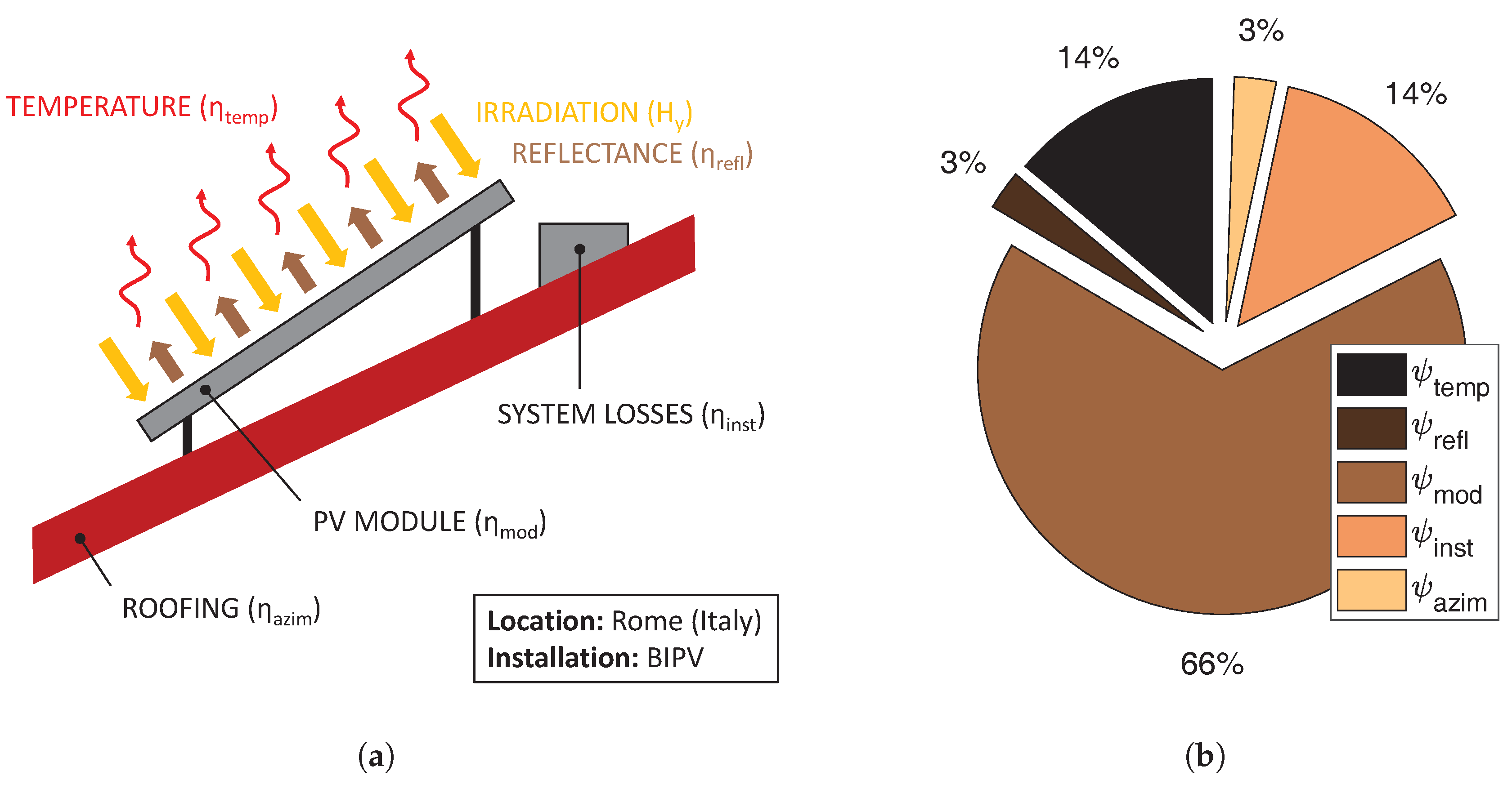
2. Methodology
3. Results
3.1. Solar Irradiation Model
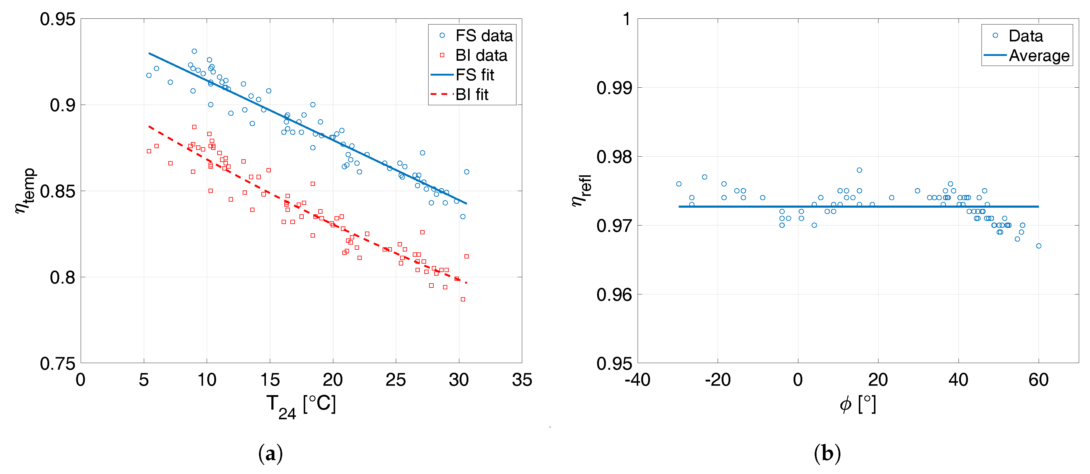
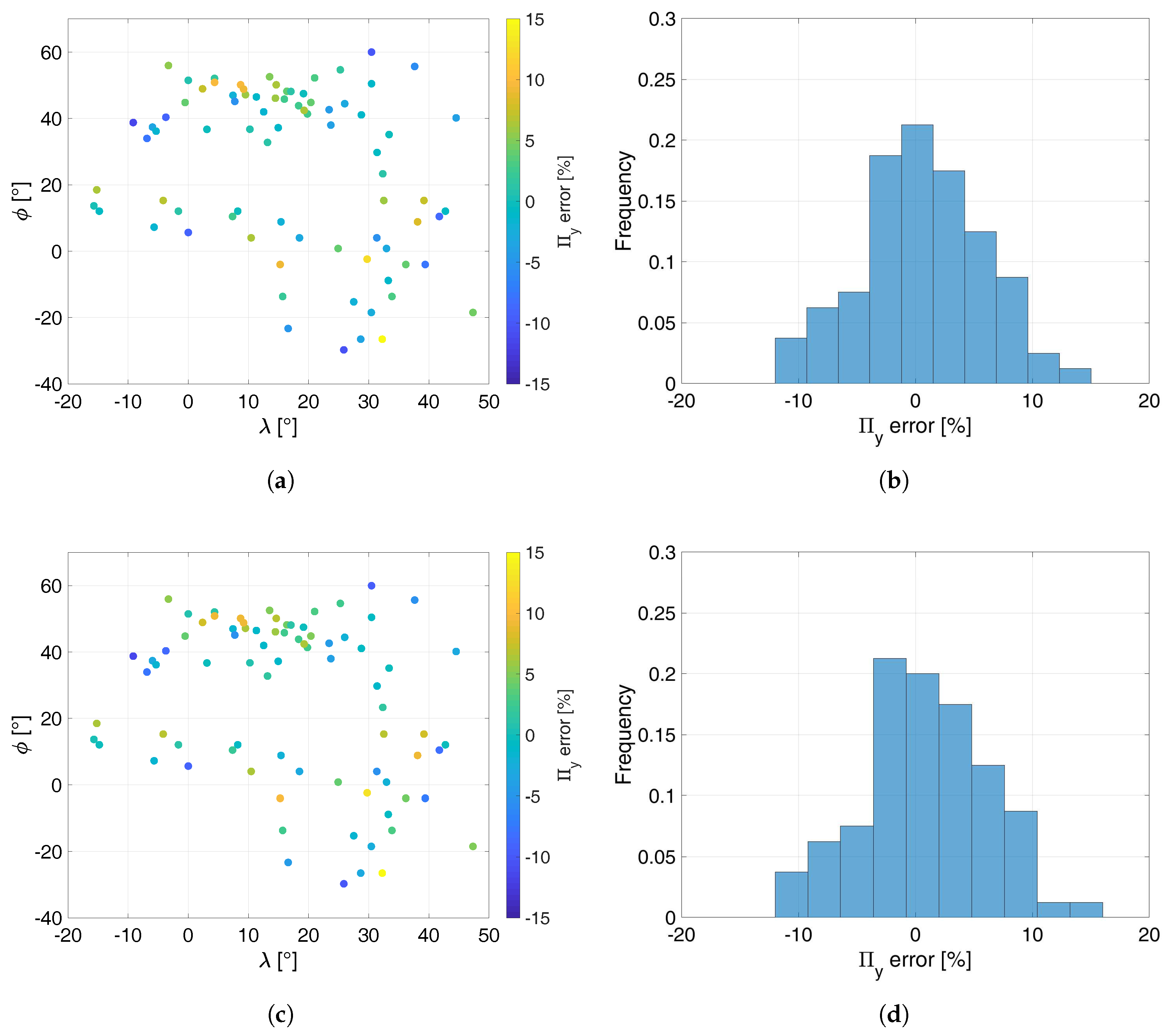
3.2. PV Energy Model (Optimal Azimuth)
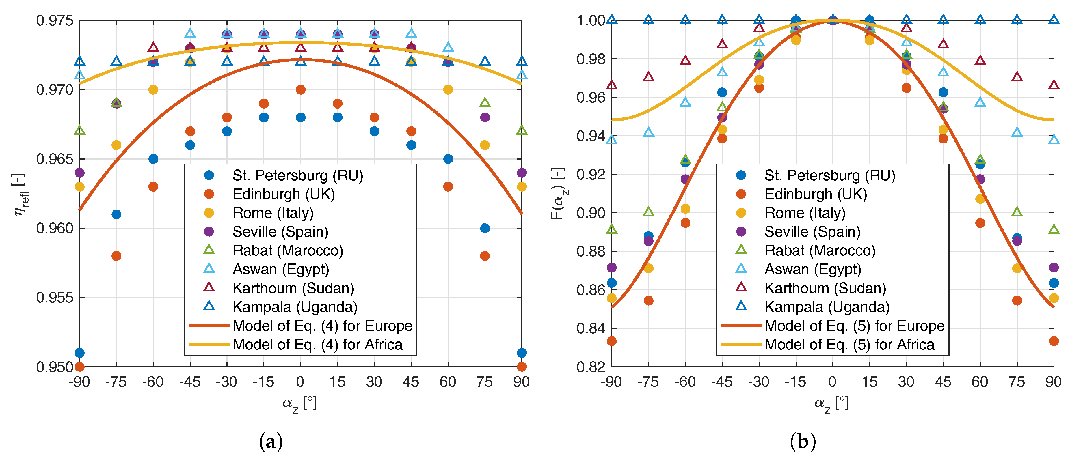
3.3. Effect of Non-Optimal Azimuth
4. Concluding Remarks
Author Contributions
Funding
Acknowledgments
Conflicts of Interest
Abbreviations
| PV | Photovoltaic |
| BIPV | Building-Integrated Photovoltaic |
| PVGIS | Photovoltaic Geographic Information System |
| JRC | Joint Research Centre (European Commission) |
| CM-SAF | Satellite Application Facility on Climate Monitoring |
| MAPE | Mean Absolute Percent Error |
| NRMSE | Normalized Root Mean Square Error |
Appendix A

| Location | Country | [] | [] | h [m] | [C] | [kWh/m2] | [%] | |
|---|---|---|---|---|---|---|---|---|
| PVGIS | Computed | |||||||
| Edinburgh | Scotland | 55.94 | −3.30 | 44 | 9.0 | 1140 | 1208 | 6.0 |
| Vilnius | Lithuania | 54.64 | 25.27 | 186 | 7.1 | 1140 | 1142 | 0.2 |
| Warsaw | Poland | 52.20 | 21.00 | 110 | 8.9 | 1240 | 1270 | 2.4 |
| London | England | 51.48 | 0.00 | 28 | 10.2 | 1320 | 1351 | 2.4 |
| Kiev | Ukraine | 50.45 | 30.46 | 165 | 8.9 | 1340 | 1306 | −2.6 |
| Prague | Czech Republic | 50.12 | 14.62 | 280 | 9.3 | 1270 | 1350 | 6.3 |
| Vienna | Austria | 48.17 | 16.39 | 223 | 11.0 | 1410 | 1476 | 4.7 |
| Budapest | Hungary | 47.47 | 19.15 | 123 | 11.5 | 1510 | 1505 | −0.3 |
| Vaduz | Liechtenstein | 47.14 | 9.50 | 454 | 10.3 | 1420 | 1477 | 4.0 |
| Bolzano | Italy | 46.47 | 11.32 | 238 | 14.1 | 1740 | 1725 | −0.8 |
| Zagreb | Croatia | 45.81 | 15.97 | 127 | 11.7 | 1500 | 1539 | 2.6 |
| Belgrade | Serbia | 44.80 | 20.38 | 80 | 13.0 | 1590 | 1633 | 2.7 |
| Bucharest | Romania | 44.43 | 26.00 | 90 | 11.9 | 1640 | 1563 | −4.7 |
| Sofia | Bulgaria | 42.63 | 23.41 | 575 | 10.3 | 1640 | 1557 | −5.1 |
| Rome | Italy | 41.97 | 12.53 | 54 | 16.4 | 1940 | 1914 | −1.3 |
| Tirana | Albania | 41.36 | 19.80 | 111 | 16.4 | 1890 | 1923 | 1.8 |
| Yerevan | Armenia | 40.16 | 44.52 | 1011 | 13.6 | 1950 | 1844 | −5.4 |
| Lisbon | Portugal | 38.75 | −9.15 | 89 | 16.3 | 2170 | 1919 | −11.6 |
| Seville | Spain | 37.38 | −5.95 | 14 | 18.4 | 2180 | 2076 | −4.8 |
| Tunisi | Tunisia | 36.74 | 10.24 | 16 | 18.6 | 2090 | 2091 | 0.0 |
| Gibraltar | Gibraltar | 36.15 | −5.35 | 4 | 17.7 | 2050 | 2017 | −1.6 |
| Rabat | Morocco | 33.96 | −6.87 | 75 | 17.5 | 2200 | 2011 | −8.6 |
| Cairo | Egypt | 29.74 | 31.38 | 96 | 22.7 | 2390 | 2368 | −0.9 |
| Aswan | Egypt | 23.31 | 32.33 | 240 | 27.4 | 2560 | 2583 | 0.9 |
| Mopti | Mali | 15.27 | −4.17 | 261 | 29.8 | 2270 | 2420 | 6.6 |
| Kaolack | Senegal | 13.66 | −15.69 | 0 | 28.6 | 2280 | 2278 | −0.1 |
| Ouagadougou | Burkina Faso | 12.05 | −1.64 | 319 | 29.0 | 2250 | 2273 | 1.0 |
| Djibouti | Republic of Djibouti | 12.05 | 42.74 | 942 | 30.6 | 2370 | 2400 | 1.3 |
| Dire Dawa | Ethiopia | 10.45 | 41.73 | 677 | 28.9 | 2490 | 2258 | −9.3 |
| Addis Ababa | Ethiopia | 8.84 | 38.11 | 2379 | 19.0 | 2140 | 2331 | 8.9 |
| Accra | Ghana | 5.63 | 0.00 | 9 | 27.1 | 2140 | 1985 | −7.2 |
| Bangui | Central African Republic | 4.02 | 18.48 | 376 | 25.5 | 2080 | 1997 | −4.0 |
| Douala | Cameroon | 4.02 | 10.45 | 327 | 25.3 | 1880 | 1992 | 5.9 |
| Kisangani | DR Congo | 0.80 | 24.91 | 445 | 25.7 | 1850 | 1923 | 3.9 |
| Mombasa | Kenya | −4.02 | 39.38 | 219 | 26.7 | 2130 | 1967 | −7.6 |
| Brazzaville | Republic of the Congo | −4.02 | 15.27 | 399 | 24.5 | 1850 | 2007 | 8.5 |
| Huambo | Angola | −13.66 | 15.69 | 1562 | 21.2 | 2260 | 2288 | 1.3 |
| Harare | Zimbabwe | −18.48 | 30.42 | 1281 | 20.8 | 2340 | 2285 | −2.3 |
| Maputo | Mozambique | −26.52 | 32.24 | 48 | 21.9 | 1990 | 2260 | 13.6 |
| Johannesburg | South Africa | −26.52 | 28.66 | 1602 | 16.1 | 2250 | 2149 | −4.5 |
| Location | Country | [] | [] | h [m] | [C] | [kWh/m2] | [%] | |
|---|---|---|---|---|---|---|---|---|
| PVGIS | Computed | |||||||
| St. Petersburg | Russia | 59.98 | 30.46 | 18 | 5.4 | 1070 | 941 | −12.1 |
| Moscow | Russia | 55.65 | 37.63 | 170 | 6.0 | 1160 | 1070 | −7.7 |
| Berlin | Germany | 52.54 | 13.52 | 55 | 9.7 | 1250 | 1307 | 4.6 |
| The Hague | Netherlands | 52.06 | 4.36 | 0 | 10.3 | 1320 | 1346 | 2.0 |
| Brussels | Belgium | 50.86 | 4.37 | 54 | 10.4 | 1250 | 1377 | 10.2 |
| Frankfurt | Germany | 50.13 | 8.70 | 133 | 10.5 | 1280 | 1404 | 9.7 |
| Paris | France | 48.91 | 2.37 | 38 | 11.4 | 1370 | 1469 | 7.2 |
| Stuttgart | Germany | 48.80 | 9.20 | 242 | 10.5 | 1320 | 1438 | 8.9 |
| Bratislava | Slovakia | 48.11 | 17.06 | 134 | 11.2 | 1460 | 1478 | 1.2 |
| Bern | Switzerland | 46.96 | 7.43 | 571 | 8.7 | 1440 | 1407 | −2.3 |
| Ljubljana | Slovenia | 46.08 | 14.48 | 311 | 11.5 | 1460 | 1547 | 6.0 |
| Turin | Italy | 45.11 | 7.73 | 210 | 12.9 | 1720 | 1641 | −4.6 |
| Bordeaux | France | 44.79 | −0.53 | 4 | 13.5 | 1600 | 1660 | 3.7 |
| Sarajevo | Bosnia-Herzegovina | 43.83 | 18.34 | 514 | 10.3 | 1500 | 1532 | 2.1 |
| Podgorica | Montenegro | 42.42 | 19.26 | 48 | 17.3 | 1880 | 1991 | 5.9 |
| Istanbul | Turkey | 41.07 | 28.77 | 90 | 14.9 | 1800 | 1803 | 0.2 |
| Madrid | Spain | 40.35 | −3.73 | 615 | 14.5 | 2040 | 1851 | −9.3 |
| Athens | Greece | 37.98 | 23.70 | 30 | 18.4 | 2120 | 2080 | −1.9 |
| Syracuse | Italy | 37.20 | 14.95 | 348 | 16.3 | 1990 | 1958 | −1.6 |
| Algiers | Algeria | 36.70 | 3.10 | 12 | 19.1 | 2140 | 2132 | −0.4 |
| Nicosia | Cyprus | 35.14 | 33.38 | 171 | 20.3 | 2240 | 2245 | 0.2 |
| Tripoli | Libya | 32.76 | 13.17 | 51 | 21.1 | 2280 | 2273 | −0.3 |
| Nouakchott | Mauritania | 18.48 | −15.21 | 12 | 28.2 | 2310 | 2437 | 5.5 |
| Karthoum | Sudan | 15.27 | 32.50 | 379 | 30.3 | 2350 | 2456 | 4.5 |
| Asmara | Eritrea | 15.27 | 39.17 | 1337 | 25.4 | 2250 | 2405 | 6.9 |
| Bafatá | Guinea Bissau | 12.05 | −14.79 | 7 | 28.0 | 2230 | 2205 | −1.1 |
| Kano | Nigeria | 12.05 | 8.22 | 514 | 27.2 | 2270 | 2255 | −0.7 |
| Kaduna | Nigeria | 10.45 | 7.36 | 589 | 26.8 | 2160 | 2208 | 2.2 |
| Moundou | Chad | 8.84 | 15.41 | 420 | 27.8 | 2230 | 2149 | −3.6 |
| Bouaflé | Côte d’Ivoire | 7.23 | −5.68 | 185 | 26.5 | 2100 | 2056 | −2.1 |
| Juba | South Sudan | 4.02 | 31.34 | 803 | 26.7 | 2180 | 2047 | −6.1 |
| Kampala | Uganda | 0.80 | 32.95 | 1075 | 24.1 | 2110 | 2038 | −3.4 |
| Ngoma | Rwanda | −2.41 | 29.73 | 1692 | 19.9 | 1970 | 2201 | 11.7 |
| Tarangire N.P. | Tanzania | −4.02 | 36.16 | 1175 | 22.1 | 2090 | 2129 | 1.8 |
| Mbeya | Tanzania | −8.84 | 33.24 | 1261 | 20.9 | 2260 | 2194 | −2.9 |
| Lilongwe | Malawi | −13.66 | 33.85 | 1438 | 20.7 | 2180 | 2260 | 3.7 |
| Lusaka | Zambia | −15.27 | 27.50 | 1030 | 21.4 | 2300 | 2238 | −2.7 |
| Antananarivo | Madagascar | −18.48 | 47.32 | 1392 | 20.0 | 2170 | 2271 | 4.7 |
| Windhoek | Namibia | −23.31 | 16.60 | 1794 | 21.5 | 2560 | 2437 | −4.8 |
| Bloemfontein | South Africa | −29.74 | 25.85 | 1411 | 16.8 | 2430 | 2152 | −11.4 |
References
- IEA World Energy Outlook 2017. Available online: http://www.iea.org/weo/ (accessed on 14 June 2018).
- Kyoto Protocol to the United Nations Framework Convention on Climate Change; U.N. Doc FCCC/CP/1997/7/ Add.1, 37 I.L.M. 22. Kyoto, Japan, 1998. Available online: http://www.globaldialoguefoundation.org/files/ENV.2009-jun.unframeworkconventionclimate.pdf (accessed on 11 December 2018).
- Huld, T.; Gracia Amillo, A.M. Estimating PV Module Performance over Large Geographical Regions: The Role of Irradiance, Air Temperature, Wind Speed and Solar Spectrum. Energies 2015, 8, 5159–5181. [Google Scholar] [CrossRef] [Green Version]
- Directive 2009/28/EC of the European Parliament and of the Council. 2009. Available online: http://data.europa.eu/eli/dir/2009/28/oj (accessed on 11 December 2018).
- Proposal for a Directive COM 2016/767/F2 of the European Parliament and of the Council. 2016. Available online: https://ec.europa.eu/transparency/regdoc/rep/1/2016/EN/COM-2016-767-F2-EN-MAIN-PART-1.PDF (accessed on 11 December 2018).
- Martínez-Rubio, A.; Sanz-Adan, F.; Santamaría-Peña, J.; Martínez, A. Evaluating solar irradiance over facades in high building cities, based on LiDAR technology. Appl. Energy 2016, 183, 133–147. [Google Scholar] [CrossRef]
- Numbi, B.P.; Malinga, S.J. Optimal energy cost and economic analysis of a residential grid-interactive solar PV system-case of eThekwini municipality in South Africa. Appl. Energy 2017, 186, 28–45. [Google Scholar] [CrossRef]
- Micangeli, A.; Del Citto, R.; Santori, S.G.; Gambino, V.; Kiplagat, J.; Viganò, D.; Poli, D.; Fioriti, D.; Del Citto, R.; Kiva, I.N. Energy Production Analysis and Optimization of Mini-Grid in Remote Areas: The Case Study of Habaswein, Kenya. Energies 2017, 10, 2041. [Google Scholar] [CrossRef]
- International Renewable Energy Agency (IRENA). Solar PV in Africa: Costs and Markets. 2016. Available online: https://www.irena.org/-/media/Files/IRENA/Agency/Publication/2016/IRENA_Solar_PV_Costs_Africa_2016.pdf (accessed on 11 December 2018).
- Quansah, D.A.; Adaramola, M.S.; Mensah, L.D. Solar Photovoltaics in sub-Saharan Africa—Addressing Barriers, Unlocking Potential. Energy Procedia 2016, 106, 97–110. [Google Scholar] [CrossRef]
- Rus-Casas, C.; Aguilar, J.D.; Rodrigo, P.; Almonacid, F.; Pérez-Higueras, P.J. Classification of methods for annual energy harvesting calculations of photovoltaic generators. Energy Convers. Manag. 2014, 78, 527–536. [Google Scholar] [CrossRef]
- Yousif, J.H.; Kazem, H.A.; Boland, J. Predictive models for photovoltaic electricity production in hot weather conditions. Energies 2017, 10, 971. [Google Scholar] [CrossRef]
- Dobos, A.P. PVWatts Version 5 Manual; Technical Report; National Renewable Energy Laboratory (NREL): Golden, CO, USA, 2014.
- Šúri, M.; Huld, T.A.; Dunlop, E.D. PV-GIS: A web-based solar radiation database for the calculation of PV potential in Europe. Int. J. Sustain. Energy 2005, 24, 55–67. [Google Scholar] [CrossRef]
- International Renewable Energy Agency (IRENA). Global Atlas for Renewable Energy: Overview of Solar and Wind Maps. 2014. Available online: https://www.irena.org/-/media/Files/IRENA/Agency/Publication/2014/GA_Booklet_Web.pdf (accessed on 11 December 2018).
- SOLARGIS. Available online: https://solargis.info/ (accessed on 14 June 2018).
- Huld, T.; Müller, R.; Gambardella, A. A new solar radiation database for estimating PV performance in Europe and Africa. Sol. Energy 2012, 86, 1803–1815. [Google Scholar] [CrossRef]
- Besharat, F.; Dehghan, A.A.; Faghih, A.R. Empirical models for estimating global solar radiation: A review and case study. Renew. Sustain. Energy Rev. 2013, 21, 798–821. [Google Scholar] [CrossRef]
- Zhang, J.; Zhao, L.; Deng, S.; Xu, W.; Zhang, Y. A critical review of the models used to estimate solar radiation. Renew. Sustain. Energy Rev. 2017, 70, 314–329. [Google Scholar] [CrossRef]
- Erbs, D.G.; Klein, S.A.; Duffie, J.A. Estimation of the diffuse radiation fraction for hourly, daily and monthly-average global radiation. Sol. Energy 1982, 28, 293–302. [Google Scholar] [CrossRef]
- Noorian, A.M.; Moradi, I.; Kamali, G.A. Evaluation of 12 models to estimate hourly diffuse irradiation on inclined surfaces. Renew. Energy 2008, 33, 1406–1412. [Google Scholar] [CrossRef]
- Perez, R.; Ineichen, P.; Seals, R.; Michalsky, J.; Stewart, R. Modeling daylight availability and irradiance components from direct and global irradiance. Sol. Energy 1990, 44, 271–289. [Google Scholar] [CrossRef]
- Skoplaki, E.; Palyvos, J.A. On the temperature dependence of photovoltaic module electrical performance: A review of efficiency/power correlations. Sol. Energy 2009, 83, 614–624. [Google Scholar] [CrossRef]
- Bocca, A.; Chiavazzo, E.; Macii, A.; Asinari, P. Solar energy potential assessment: An overview and a fast modeling approach with application to Italy. Renew. Sustain. Energy Rev. 2015, 49, 291–296. [Google Scholar] [CrossRef] [Green Version]
- Bocca, A.; Bottaccioli, L.; Chiavazzo, E.; Fasano, M.; Macii, A.; Asinari, P. Estimating photovoltaic energy potential from a minimal set of randomly sampled data. Renew. Energy 2016, 97, 457–467. [Google Scholar] [CrossRef]
- Pfenninger, S.; Staffell, I. Long-term patterns of European PV output using 30 years of validated hourly reanalysis and satellite data. Energy 2016, 114, 1251–1265. [Google Scholar] [CrossRef]
- Pfenninger, S. Dealing with multiple decades of hourly wind and PV time series in energy models: A comparison of methods to reduce time resolution and the planning implications of inter-annual variability. Appl. Energy 2017, 197, 1–13. [Google Scholar] [CrossRef]
- Bergamasco, L.; Asinari, P. Scalable methodology for the photovoltaic solar energy potential assessment based on available roof surface area: Application to Piedmont Region (Italy). Sol. Energy 2011, 85, 1041–1055. [Google Scholar] [CrossRef] [Green Version]
- Bergamasco, L.; Asinari, P. Scalable methodology for the photovoltaic solar energy potential assessment based on available roof surface area: Further improvements by ortho-image analysis and application to Turin (Italy). Sol. Energy 2011, 85, 2741–2756. [Google Scholar] [CrossRef] [Green Version]
- ESRI World Imagery. Available online: https://www.arcgis.com/ (accessed on 14 June 2018).
- Duffie, J.A.; Beckman, W.A. Solar Engineering of Thermal Processes; John Wiley & Sons: Hoboken, NJ, USA, 2013. [Google Scholar]
- Aldobhani, A.A.M.S. Effect of Altitude and Tilt Angle on Solar Radiation in Tropical Regions. J. Sci. Technol. 2014, 19, 96–109. [Google Scholar]
- Wong, L.; Chow, W. Solar radiation model. Appl. Energy 2001, 69, 191–224. [Google Scholar] [CrossRef]
- Dubey, S.; Sarvaiya, J.N.; Seshadri, B. Temperature Dependent Photovoltaic PV Efficiency and Its Effect on PV Production in the World—A Review. Energy Procedia 2013, 33, 311–321. [Google Scholar] [CrossRef]
- Bocca, A.; Bottaccioli, L.; Macii, A. Temperature Efficiency Analysis in Photovoltaics Using Basic Geodata: Application to Europe. In Proceedings of the 2018 International Symposium on Power Electronics, Automation and Motion (SPEEDAM), Amalfi, Italy, 20–22 June 2018; pp. 823–828. [Google Scholar]
- Martin, N.; Ruiz, J.M. Calculation of the PV modules angular losses under field conditions by means of an analytical model. Sol. Energy Mater. Sol. Cells 2001, 70, 25–38. [Google Scholar] [CrossRef]
- PVGIS, Online Tool. Available online: http://re.jrc.ec.europa.eu/pvgis (accessed on 14 June 2018).
- Šúri, M.; Huld, T.; Dunlop, E.; Ossenbrink, H. Potential of solar electricity generation in the European Union member states and candidate countries. Sol. Energy 2007, 81, 1295–1305. [Google Scholar] [CrossRef]
- Gracia Amillo, A.M.; Huld, T. Performance Comparison of Different Models for the Estimation of Global Irradiance on Inclined Surfaces. Validation of the Model Implemented in PVGIS; Technical Report EUR 26075 EN, JRC81902; 2013; ISBN 978-92-79-32507-6. Available online: https://publications.europa.eu/en/publication-detail/-/publication/4ef8c4e1-4397-4e27-8487-448786327f27 (accessed on 11 December 2018).
- Urraca, R.; Gracia-Amillo, A.M.; Koubli, E.; Huld, T.; Trentmann, J.; Riihelä, A.; Lindfors, A.V.; Palmer, D.; Gottschalg, R.; Antonanzas-Torres, F. Extensive validation of CM SAF surface radiation products over Europe. Remote Sens. Environ. 2017, 199, 171–186. [Google Scholar] [CrossRef] [Green Version]
- Berkeley Earth. Available online: http://berkeleyearth.lbl.gov (accessed on 12 September 2018).
- Zhang, J.; Hodge, B.M.; Florita, A.; Lu, S.; Hamann, H.F.; Banunarayanan, V. Metrics for Evaluating the Accuracy of Solar Power Forecasting. In Proceedings of the 3rd International Workshop on Integration of Solar Power into Power Systems, London, UK, 21–22 October 2013; pp. 1–19. [Google Scholar]
- Taylor, B.N.; Thompson, A. The International System of Units (SI)—NIST Special Publication 330; National Institute of Standards and Technology: Gaithersburg, MD, USA, 2008.
- Šúri, M.; Cebecauer, T.; Skoczek, A. SolarGIS: Solar data and online applications for PV planning and performance assessment. In Proceedings of the 26th European Photovoltaics Solar Energy Conference, Hamburg, Germany, 5–9 September 2011. [Google Scholar]
- Global Solar Atlas: Accuracy. Available online: http://globalsolaratlas.info/knowledge-base/accuracy? (accessed on 12 September 2018).
- Khatib, T.; Mohamed, A.; Sopian, K.; Mahmoud, M. Solar energy prediction for Malaysia using artificial neural networks. Int. J. Photoenergy 2012, 2012, 419504. [Google Scholar] [CrossRef]
- Rumbayan, M.; Abudureyimu, A.; Nagasaka, K. Mapping of solar energy potential in Indonesia using artificial neural network and geographical information system. Renew. Sustain. Energy Rev. 2012, 16, 1437–1449. [Google Scholar] [CrossRef]
- Kuo, P.H.; Chen, H.C.; Huang, C.J. Solar Radiation Estimation Algorithm and Field Verification in Taiwan. Energies 2018, 11, 1374. [Google Scholar] [CrossRef]
- Williams, S.R.; Gottschalg, R. Accuracy of European Energy Modelling Approaches. In Proceedings of the 21st European Photovoltaic Solar Energy Conference, Dresden, Germany, 4–8 September 2006; pp. 2452–2455. [Google Scholar]
- Green, M.A.; Hishikawa, Y.; Dunlop, E.D.; Levi, D.H.; Hohl-Ebinger, J.; Ho-Baillie, A.W.Y. Solar cell efficiency tables (version 51). Prog. Photovolt. Res. Appl. 2017, 26, 3–12. [Google Scholar] [CrossRef] [Green Version]
- Aderemi, B.; Chowdhury, S.; Olwal, T.; Abu-Mahfouz, A. Techno-Economic Feasibility of Hybrid Solar Photovoltaic and Battery Energy Storage Power System for a Mobile Cellular Base Station in Soshanguve, South Africa. Energies 2018, 11, 1572. [Google Scholar] [CrossRef]
- Gueymard, C. Prediction and performance assessment of mean hourly global radiation. Sol. Energy 2000, 68, 285–303. [Google Scholar] [CrossRef]
- Rose, A.; Stoner, R.; Pérez-Arriaga, I. Prospects for grid-connected solar PV in Kenya: A systems approach. Appl. Energy 2016, 161, 583–590. [Google Scholar] [CrossRef]
- Mohan, G.; Kumar, U.; Pokhrel, M.K.; Martin, A. A novel solar thermal polygeneration system for sustainable production of cooling, clean water and domestic hot water in United Arab Emirates: Dynamic simulation and economic evaluation. Appl. Energy 2016, 167, 173–188. [Google Scholar] [CrossRef]
- Pintér, G.; Baranyai, N.H.; Wiliams, A.; Zsiborács, H. Study of Photovoltaics and LED Energy Efficiency: Case Study in Hungary. Energies 2018, 11, 790. [Google Scholar] [CrossRef]
- Zsiborács, H.; Baranyai, N.H.; Vincze, A.; Háber, I.; Pintér, G. Economic and Technical Aspects of Flexible Storage Photovoltaic Systems in Europe. Energies 2018, 11, 1445. [Google Scholar] [CrossRef]
- Morciano, M.; Fasano, M.; Secreto, M.; Jamolov, U.; Chiavazzo, E.; Asinari, P. Installation of a concentrated solar power system for the thermal needs of buildings or industrial processes. Energy Procedia 2016, 101, 956–963. [Google Scholar] [CrossRef]
- Marucci, A.; Cappuccini, A. Dynamic photovoltaic greenhouse: Energy efficiency in clear sky conditions. Appl. Energy 2016, 170, 362–376. [Google Scholar] [CrossRef]
- Morciano, M.; Fasano, M.; Salomov, U.; Ventola, L.; Chiavazzo, E.; Asinari, P. Efficient steam generation by inexpensive narrow gap evaporation device for solar applications. Sci. Rep. 2017, 7, 11970. [Google Scholar] [CrossRef] [Green Version]


| Parameter | Average Value | Standard Deviation |
|---|---|---|
| [kWh·m] | −21.569 | ±2.073 |
| [kWh·m] | 0.137 | ±0.031 |
| [kWh·mC] | −0.421 | ±0.133 |
| [kWh·mC] | 0.071 | ±0.003 |
| [kWh·m] | 2119.345 | ±108.680 |
| Parameter | Free-Standing | Building-Integrated |
|---|---|---|
| [C] | ||
| [C] | ||
| [−] |
© 2018 by the authors. Licensee MDPI, Basel, Switzerland. This article is an open access article distributed under the terms and conditions of the Creative Commons Attribution (CC BY) license (http://creativecommons.org/licenses/by/4.0/).
Share and Cite
Bocca, A.; Bergamasco, L.; Fasano, M.; Bottaccioli, L.; Chiavazzo, E.; Macii, A.; Asinari, P. Multiple-Regression Method for Fast Estimation of Solar Irradiation and Photovoltaic Energy Potentials over Europe and Africa. Energies 2018, 11, 3477. https://doi.org/10.3390/en11123477
Bocca A, Bergamasco L, Fasano M, Bottaccioli L, Chiavazzo E, Macii A, Asinari P. Multiple-Regression Method for Fast Estimation of Solar Irradiation and Photovoltaic Energy Potentials over Europe and Africa. Energies. 2018; 11(12):3477. https://doi.org/10.3390/en11123477
Chicago/Turabian StyleBocca, Alberto, Luca Bergamasco, Matteo Fasano, Lorenzo Bottaccioli, Eliodoro Chiavazzo, Alberto Macii, and Pietro Asinari. 2018. "Multiple-Regression Method for Fast Estimation of Solar Irradiation and Photovoltaic Energy Potentials over Europe and Africa" Energies 11, no. 12: 3477. https://doi.org/10.3390/en11123477