Operational Planning and Bidding for District Heating Systems with Uncertain Renewable Energy Production


1
Department of Applied Mathematics and Computer Science, Technical University of Denmark, Richard Petersens Plads, 2800 Kgs. Lyngby, Denmark
2
EMD International A/S, Niels Jernesvej 10, 9220 Aalborg Ø, Denmark
*
Author to whom correspondence should be addressed.
Energies 2018, 11(12), 3310; https://doi.org/10.3390/en11123310
Submission received: 24 October 2018
/
Revised: 15 November 2018
/
Accepted: 21 November 2018
/
Published: 27 November 2018
Abstract
:In countries with an extended use of district heating (DH), the integrated operation of DH and power systems can increase the flexibility of the power system, achieving a higher integration of renewable energy sources (RES). DH operators can not only provide flexibility to the power system by acting on the electricity market, but also profit from the situation to lower the overall system cost. However, the operational planning and bidding includes several uncertain components at the time of planning: electricity prices as well as heat and power production from RES. In this publication, we propose a planning method based on stochastic programming that supports DH operators by scheduling the production and creating bids for the day-ahead and balancing electricity markets. We apply our solution approach to a real case study in Denmark and perform an extensive analysis of the production and trading behavior of the DH system. The analysis provides insights on system costs, how DH system can provide regulating power, and the impact of RES on the planning.
1. Introduction
To achieve the decarbonization of the energy sector, several countries especially in the European Union started to consider district heating (DH) and cooling systems for CO-emission reduction strategies [1]. Since it is assumed that fossil fuels will be mostly replaced by intermittent renewable energy sources (RES), DH and cooling systems can facilitate a larger share of intermittent energy sources in the energy mix following the concept of integrated energy systems [2]. DH systems are able to contribute to the grid balancing by the use of flexible heat and power production, power-to-heat technologies and thermal storages.
The efficiency of DH systems has been demonstrated already in countries in northern Europe. In Denmark, more than 60% of the heat consumption is delivered by DH [3], and there exists a total of approximately 400 DH systems. The major part of those are small/medium DH systems that are usually operated based on a portfolio of different units such as combined heat and power (CHP) units (e.g., gas engines), fuel boilers, and power-to-heat technologies such as electric boilers and heat pumps. Furthermore, the installation of large solar thermal facilities (≥1000 ) in Denmark has increased significantly during the last few years, and it is expected that 20% of the total heat consumption will be covered by solar heating in 2025 [4]. Furthermore, the wider spread of power-to-heat technologies and decentralization of power production enables DH providers to include renewable power production, e.g., in the form of wind farms, in their portfolio. Although the primary goal of the DH operator is to fulfill the heat demand in the DH network at the lowest cost, selling the power production from the CHP units or other RES as well as buying the power for heat-to-power technologies on electricity markets offers the potential for additional income, resulting in lower total operating costs. However, as the RES production in the power and heat systems depends on weather conditions, the operation and planning have to deal with increased complexity and uncertainty, which requires advanced modeling techniques [5]. Moreover, the significant integration of RES and the stronger interconnection between countries led to uncertain long-term electricity price forecasts [6]. Long-term price forecasts drastically affect the investment decisions for the installation of new heat production technologies [7]. Consequently, the operation of DH systems should be robust against uncertain electricity prices to incentivize the investment and use of DH systems. Therefore, bidding methods must account for uncertain electricity prices and RES production.
In this publication, we pursue two main objectives. First, we propose an operational planning method for DH operators coping with the complexity of a system with several traditional and RES production units. This includes the bidding in two electricity markets, namely the day-ahead and balancing market. Our approach is based on the methodology presented in [8], which uses stochastic programming to account for the uncertainty of electricity prices in the operation of virtual power plants (VPPs) when creating price-dependent bids. Second, we use the proposed method to analyze the real case of a DH system in Hvide Sande, Denmark. The analysis investigates among others the behavior of the DH system in different situations, the influence of uncertainty in the RES production, and benefits from including RES power production. The results offer several insights on how DH systems should operate and can benefit in future systems with high shares of RES.
1.1. Description of Electricity Markets
Currently, the integration of the power and DH system is achieved through the participation of the latter in the electricity markets. Before describing the related work, we want to recall the concepts of the day-ahead and balancing electricity markets that are considered by the proposed planning method.
In most of the EU countries, the short-term trading of electricity is organized in a similar way. Most of the power volume is traded one day before the energy is delivered in the so-called day-ahead market. To ensure enough backup generation, producers can also bid offers in the reserve capacity market, which takes place usually also one day before the delivery of energy. Getting closer to the time of delivery, intra-day markets are organized throughout the day to help RES producers submit more accurate power production offers. The purpose of these markets is to correct the imbalances produced by RES, allowing producers to reformulate their bids. Finally, balancing markets are organized each hour of the day with gate closure one hour before the energy delivery.
Balancing markets are slightly different from intra-day markets and take place shortly before the hour of energy delivery. The balancing markets are cleared by the transmission system operator (TSO), and their goal is to provide flexibility for the operation of the system and not to the producers, as is the case for the intra-day market. Balancing prices are highly volatile and quite unpredictable even for the following hour. In addition, balancing offers are just activated in case the TSO has the need for regulation. In the case that there is a lack of power production due to a failure of a unit or an unpredictable demand, the TSO will activate offers for upward regulation, paying producers to increase the production of their power plants. On the contrary, if there is more power production than expected due to an excess of RES production, the TSO will activate downward regulation offers for producers to deactivate the production they had previously scheduled in the day-ahead market or incentivize more power consumption.
To operate efficiently in these markets, producers and consumers are allowed to submit price-dependent bids. These type of bids consist of pair-wise points of power volume and power prices that must follow a merit ascending or descending order. In this way, producers and consumers are able to provide a wider range of offers to hedge against the uncertain electricity prices. In this work, we focus on day-ahead and balancing markets.
1.2. Related Work
As mentioned before, the integration of heat and power production units complicates the operation of the system, requiring suitable tools. Among other techniques, mixed integer linear programming (MILP) has been shown as one well-suited approach to optimize the operation of DH systems. To provide some examples, the authors in [9] proposed a unit commitment model that optimizes the integration of a solar collector in a DH system that includes one fuel boiler and one CHP unit connected to a thermal storage tank. Furthermore, the authors in [10] worked with a DH system that includes several CHP units, fuel boilers, thermal storage, as well as a solar thermal plant. The authors propose an optimization model that accounts for the synchronization of the operation of the units providing an extensive analysis of the flexibility between units. Finally, the authors in [11] went a step further by introducing a wind farm in a DH system that can feed both a heat pump and the power grid. To provide flexibility to the system, they also integrated a CHP unit and a thermal storage that increased the complexity of the operating the system. All these presented publications have in common that they operate a portfolio of distributed generators and flexible loads.
Apart from the operational planning, planning methods have to consider the bidding in electricity markets. Currently, a widespread approach in practice is that producers base their offers on the given electricity price forecast, which is very volatile due to the variability of RES production and uncertain one day before the energy is delivered [12]. Additionally, the production from RES in the DH system itself is uncertain. Consequently, tools that optimize the operation of DH systems and propose bidding strategies need to consider the uncertainty given by price and production. Despite several bidding strategies for price-taker power producers in the day-ahead market have been proposed (see the references in [13]), the authors in [8] demonstrated that under high uncertainty of electricity prices, the use of stochastic programming [14] for creating bidding curves for the day-ahead market renders good solutions that consider the uncertainty involved in the bidding process. Based on the representation of the uncertain electricity prices as scenarios, the authors used non-anticipativity constraints that order the bids presented to the market in a step-wise manner to create price-dependent bids.
The above-mentioned methods consider power production only. Hence, they are not directly applicable for DH operators, as the heat production is neglected. The heat production is an important part, and a planning method needs to ensure heat demand fulfillment as well as consider the limitations of the production units and storages. Therefore, bidding methods for systems with a connected DH system need to model the heat production, as well. For example, the method proposed in [15] determines the optimal production of a CHP unit. The bidding price is the price forecast, which is the same price used to determine the power production. In [16], the authors proposed a bidding strategy for CHP units that takes into account other heat units to define the heat production costs to determine the bidding price. Finally, the authors in [17] apply the bidding strategy of [8] for the day-ahead market using stochastic programming for a DH system that includes one CHP unit, a peak boiler, and one heat storage tank.
The methods presented so far focus on the day-ahead market trading only. The consideration of bidding in sequential markets was considered, e.g., in [18], who created bids using stochastic programming in both day-ahead and intra-day markets for an aggregator, combining decentralized RES production and consumption without any connection to DH systems. The presented approach first creates bids for the day-ahead market. After this market is cleared, the already committed power production or consumption in the day-ahead market is used to formulate optimal bids for each intra-day market auction throughout the day. Additionally, the standalone participation of different units in sequential electricity markets (especially day-ahead and balancing markets) has been widely discussed in the literature (see for instance these sequence bidding strategies for thermal generators [19], microgrids [20], wind farms [21], hydropower [22], or CHP units [23]).
To the best of our knowledge, we see a research gap regarding the optimal participation of DH systems in a sequential electricity market structure using a realistic framework that includes bidding strategies. There is a need for a planning method that allows DH operators with a portfolio of units to schedule their production under uncertainty and participate in both day-ahead and balancing markets. In particular, for the case when the DH system contains CHP units, power-to-heat technologies and potentially RES power production, which offer the opportunity to lower the heat production costs by trading on the markets. The consideration of all units as portfolio hedges against the uncertain RES production and resembles the concept of a VPP power producer. However, the operational planning and bidding method needs to account for the limitations of the heat production with respect to demand and thermal storages. Such a method offers the opportunity to analyze the optimal production behavior of DH systems in a context with RES production. The contributions of this paper can be summarized as follows:
- The above-mentioned gap is addressed by extending the VPP bidding method of [8], which only considers power production, to a DH setting. Furthermore, we add a second model to optimize the trading on the balancing market after the day-ahead market is cleared. The underlying stochastic programs for modeling the operation of the DH system are formulated in a general manner to be applicable to arbitrary sets of production units in DH systems.
- In contrast to previous work, the method explicitly accounts for the uncertainty coming from RES production in both heat and power and enables us to perform an analysis of the impact of the different uncertainty sources.
- The method is analyzed using a real case study based on the Hvide Sande DH system in Denmark that allows us to draw conclusions on: (a) the behavior of the system under uncertain RES production; (b) the impact of including balancing market trading in the planning method; (c) the benefits of including renewable power production in the portfolio; and (d) the annual system costs compared to traditional bidding methods based on forecasts.
- An additional contribution is a new approach to generate scenarios for balancing market price scenarios needed for the stochastic programming, addressing the balancing market-related operation.
Our study is based on the following assumptions. First, we assume the DH operator is a price-taker, i.e., we do not influence the market price, which is reasonable for small- and medium-sized DH systems. Second, we assume that the markets allow the submission of price-dependent bids, as is the case in Nord Pool. Third, we do not consider minimum and maximum power volume restrictions in either market. Fourth, we assume electricity prices and RES production are uncertain when planning the day-ahead bidding. For the balancing bids, we consider the RES production known for the next hour. The heat demand is assumed to be known and adjusted to cover the heat losses. The reason we consider heat demand as a known parameter is due to its strong correlation with the ambient temperature and season of the year. Thus, having previous observations, we can obtain very accurate predictability 24 h ahead [24]. In addition, if a particular deviation from the predicted heat demand occurs, the DH operators have mechanisms to correct these imbalances such as increasing or decreasing the pressure in the DH network. Finally, we do not consider wind spillage as a recourse variable, and therefore, we are responsible for our own imbalances.
The remainder of this paper is organized as follows. In Section 2, we provide the mathematical formulation that describe the two operational problems for day-ahead and balancing market, respectively. Section 3 describes the modeling of uncertainty, i.e., the scenario generation for the RES production and electricity prices. Section 4 describes the bidding strategy. The Hvide Sande case study is described in detail in Section 5. Section 6 provides an analysis and discussion of the results obtained for the case study. Finally, Section 7 summarizes our work and gives an outlook on future work.
2. Operational Planning Model
We start by introducing the two-stage stochastic programs that are the basis for creating bids for the day-ahead and balancing market. The major part of the constraints is valid for both markets and relates to the operation of a portfolio of production units in a DH system. We start by introducing those constraints. The specific constraints and objectives regarding the two different markets are given in Section 2.1 and Section 2.2 for day-ahead and balancing market, respectively. For an overview of the nomenclature, we refer to Table 1.
The overall goal is to fulfill the heat demand in the DH network in each period of time at the lowest cost while taking expected income from bids won on the electricity markets into account. The DH operator has a set of heat and power production units that are operated as a portfolio. We divide the set of units into heat producing units and intermittent renewable power-only production units (wind power or photo-voltaic). The heat-producing units are further categorized into CHP plants (producing heat and power simultaneously at a heat-to-power ratio ), heat-only units using electricity , heat-only units with controllable production based on other fuels , and stochastic heat production units (e.g., solar thermal). The stochastic production of both heat and power units is modeled based on a set of scenarios given by the parameters and , respectively. Each of the heat-producing units has a lower and upper limit on the production amount per period given by and .
The DH operator further uses thermal storages to store heat over several periods. The minimum and maximum level of each storage are denoted by and , whereas the initial level is set by . The physical connections of the units to the storages and the DH network are modeled by the binary parameters and , respectively (equals one, if a connections exists, and zero otherwise).
The operational cost for producing one MWh of heat are represented by the coefficients . A special case is the production of heat based on electricity, i.e., the units have additional costs on top of the operational cost based on the electricity needed. We consider a special tariff for producing heat with heat units fueled by power produced by our own power generators . Electricity bought from the grid for units is included in the bids to the market. The income from the market is approximated based on the amount of power offered to the market and electricity price scenarios .
The decisions determined by the model are the production amounts of heat () and power () for the dispatchable units as well as the amount of power offered to the electricity market, the latter being the first-stage decisions in our stochastic program. Further variables relate to the storage and feeding to the DH and are described later. All variables and their domains are given in Table 1.
The following constraints are valid for the production scheduling on both a day-ahead market and balancing market level. The heat production of each unit is limited to the capacities of the unit by constraints (1a). In constraints (1b), the production of each unit is split into heat used in the DH network () and heat stored in the thermal storage (). The possibility of this split is dependent on the existing connections to storages and the DH network. Flow in non-existent connections is avoided by constraints (1c) and (1d).
The coupling of heat and power production in CHP units is modeled in constraints (1e). Furthermore, the electric boiler production can be based on electricity bought on the market () or from our own power generators () (see constraints (1f)). Stochastic renewable heat production from, e.g., solar thermal units is dependent on the scenario and given as input in constraints (1g).
The thermal storage level () limitations as well as in- and out-flows () are modeled in constraints (1h) and (1i), respectively. At the end of the planning horizon, we impose that the storage level is at least as high as in the beginning of the planning horizon to avoid emptying the storage in every optimization (constraints (1j)).
The heat demand in the network in each period is ensured by constraints (1k) by using either heat directly from the units or from the storage.
The renewable power production from the stochastic power generators is modeled in constraints (1l), depending on the scenario. The power can be used either to produce heat with the power-to-heat units () or sold on the market ().
Based on this initial set of constraints, the model is extended for day-ahead or balancing market optimization in the succeeding sections.
2.1. Optimization for the Day-Ahead Market
The first-stage variables (here-and-now decisions) for the day-ahead market production scheduling are the power bids for each hour of the next day . As these are dependent on the production of all other dispatchable units, we determine the heat () and power production () of all units as well as the power bid amounts for the remaining planning horizon () as second-stage variables.The objective function (2a) minimizes the expected cost of producing heat by all units minus the expected income for the day-ahead electricity market. Deviations from the day-ahead market bid are penalized by paying the imbalances () at the balancing stage.
The bidding amount is dependent on the power production from CHP units and the generator as well as the power used for the electric boiler (see constraints (2b)). Any deviations from the bidding amount are captured in the variables and to be penalized in the objective function.
Equation (2c) are based on the method in [8] and ensure that only one bidding curve, i.e., one set of power amount and price pairs, is created per time period t, while constraints (2d) ensure that the bidding curves are non-decreasing for all time steps .
The operational model to optimize the production for the day-ahead market bidding can be summarized as follows in (3a)–(3c).
To avoid speculation in the operation of the system, we define the penalty costs for deviation as follows.
where is a parameter with a value greater than zero. Thus, we ensure that the penalty to pay would be higher than the day-ahead prices in the case of positive deviation. On the contrary, in the case of producing more power than sold in the day-ahead market, the profits for selling that excess power on the balancing market are always lower than selling that energy in the day-ahead market. Therefore, the model tries to sell the right amount of power on the day-ahead market and avoid imbalances.
2.2. Optimization for the Balancing Market
The balancing market problem is solved once per hour, and like in the day-ahead problem (3a)–(3c), we generate non-decreasing bidding curves using the stochastic formulation of the problem. In this case, the first-stage decisions are the upward () and downward () regulation offered to formulate the bidding curves for the balancing market. The remaining variables can be adapted to the realization of the uncertainty and considered as second-stage decisions. In this formulation of the balancing problem, the committed power production or consumption for the day ahead is given as a parameter (). Due to the high unpredictability of the balancing prices, we use periods as the planning horizon for the balancing problem, which can be shorter than the horizon used in the day-ahead problem. Upward regulation () is provided in case there is a need for more power in the system; therefore, the producer has the opportunity to sell additional power at the upward regulating price (). On the contrary, if the system has an excess of production, the TSO activates offers for downward regulation, where producers can consume power () at the downward regulating price ().
The objective function (4a) for the balancing problem again minimizes the cost considering income from the market and penalties for imbalances.
The balance in the power production is ensured in equations (4b). Here, the power committed on the day-ahead market is given as a parameter (). To balance the production with the bidding amount, constraints (4b) can either use the variables determining the upward () or downward regulation () amounts or pay imbalances. The imbalances are captured in and .
To ensure ordered bidding curves in the balancing market, we define constraints (4c) and (4f) analogously to the day-ahead market problem. Here, the offers for upward regulation and downward regulation present a non-decreasing and non-increasing order, respectively.
Furthermore, as in the day-ahead problem, we need to prohibit speculation of the system by defining the penalty prices and as follows.
3. Modeling Uncertainty
In particular, the day-ahead market optimization includes uncertainty with respect to the production of the stochastic production units (wind power and solar thermal). However, both planning problems also have to consider that the electricity prices are still unknown at the time of planning. To account for these uncertainties, we include them as scenarios in our two-stage stochastic programs. The remainder of this section describes the forecasting and scenario generation process.
3.1. Wind Power Production Forecast
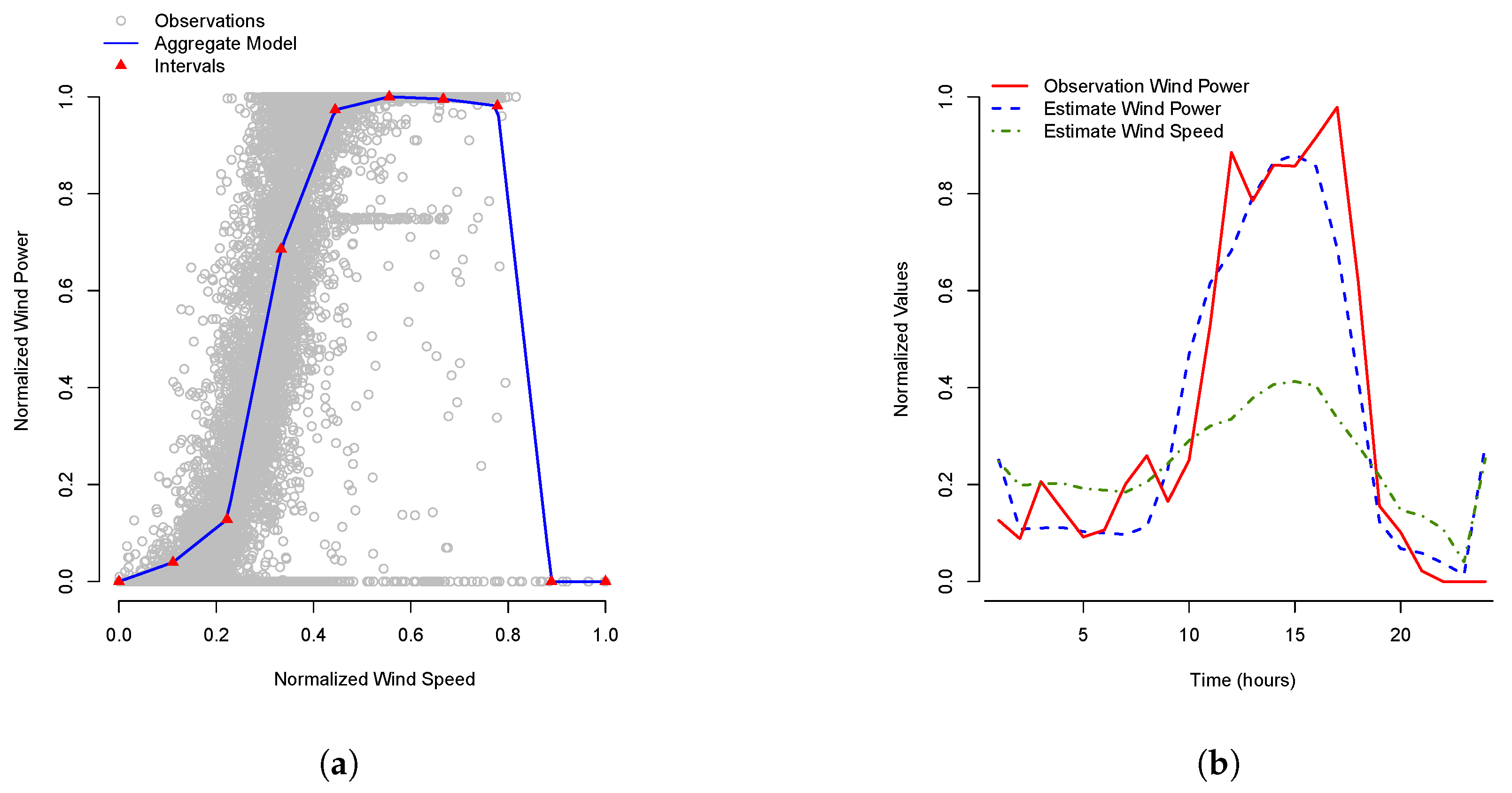
For the easy replicability of our experiments, we use a wind forecast based on local linear regressions of the wind power curve [25]. As Figure 1a shows, the power curve is divided into intervals with equal distribution based on the normalized wind speed. For each interval, a linear regression is fitted to the data using a least squares estimate. The linear regressions are later integrated into one single function. From this aggregated function, we can predict the wind power production using the wind speed forecast, as depicted in Figure 1b.
3.2. Solar Thermal Forecast
The appropriate function to predict solar thermal forecast depends on the technology used in the solar collectors. In this work, we consider flat thermal solar collectors with a fixed inclination angle and orientated towards maximizing the solar radiation during the summer season. The forecasting technique used here is presented in [26] and given in (6).
where is the heat production at time t, is the area of the entire solar thermal field, and is the solar radiation (including direct and diffusive) that heats the solar collectors for time period t. and are the average temperature inside the solar collector and the outside temperature, respectively. The remaining parameters (,,) are the coefficients of the equations. The average temperature () is defined as the average between the cold water entering and the hot water leaving the solar collector. For the sake of simplicity, we consider this temperature as constant .
3.3. Day-Ahead Electricity Price Forecast
Electricity prices in day-ahead markets present an autocorrelation and seasonal variation that usually can be detected using time series models. For this work, the electricity price forecast is obtained using a SARMAX (seasonal autoregressive moving average with exogenous terms) model with a daily seasonality pattern that has been successfully applied to predict electricity prices [27]. In addition, an exogenous variable based on Fourier series is used to describe the weekly seasonality [28]. This results in the following model (7a).
The estimated electricity price () for time period t is calculated by the linear combination of the intercept , the autoregressive (AR) terms , and , and the moving average (MA) terms , and for 1, 2 and 24 hours prior to time period t. The forecast parameters , , , , and are updated on a daily basis. The exogenous variable X allows integrating external variables into the model, in our case the Fourier series describing the weekly seasonality of the data (7b).
where K determines the number of Fourier terms considered (chosen by minimizing the AICc value). The parameter T represents the seasonality period in the series; in our case, we consider a weekly seasonality of . Finally, and represent the forecast parameters for the weekly seasonality, and like the forecast parameters for the AR and MA terms, both are updated on a daily basis.
3.4. Scenario Generation for RES Production and Day-Ahead Market Prices
The forecasts for the three previously-mentioned datasets are based on probabilistic forecasts. Therefore, we generate scenarios using a Monte-Carlo simulation applying a multivariate Gaussian distribution with zero mean that describes the stochastic process, which we consider as stationary, in our predictions. We use the algorithm presented in [29] to initialize the scenario generation process and randomly generate the error terms. The algorithm is repeated for each time period in the receding horizon and for all scenarios. In our case, we generate a random walk for the time horizon using normalized white noise that we iteratively add to the predicted value resulting in one scenario.
To get a representative set of scenarios, we generate a large amount of equiprobable scenarios. Those are reduced to the desired number by applying the clustering technique partition around medoids (PAM) [30]. Each medoid scenario is a scenario in our model, while the probability is obtained by the sum of the scenarios attached to the medoid.
3.5. Scenario Generation for Balancing Prices
The generation of scenarios for balancing prices is less intuitive compared to the day-ahead market prices described before. In particular, there is not always a need for upward or downward regulation, and if there is, the regulating prices are defined as a function of the imbalanced power volume, which makes these prices very hard to predict. The method proposed in [31] is widely used in the literature to create balancing price forecasts. The authors developed a model that combines a SARIMA (seasonal autoregressive integrated moving average) model to predict the amount of upward and downward regulating prices in combination with a discrete Markov model representing the discontinuous variability in the activation of upward and downward regulation. This variability is represented through a matrix that indicates the transition probability between states. Using this techniques, scenarios can be generated by sampling the error term in the time series models and creating different sequences for the Markov model.
In this section, we propose a novel approach to generate balancing price scenarios. Our motivation to use a different new scenario generation technique for real-time balancing prices is due to the fact that the authors in [31] applied their method in a specific bidding area where prices follow a regular shape and pattern that can be accurately predicted, i.e., regions with low integration of RES. In systems with a high penetration of RES (especially wind power), large imbalances can occur in a very short time and thereby affect the balancing prices, which respond to the volume of the imbalance. Due to this variability, balancing prices do not necessarily follow a trend that can be easily predicted using time series models. Furthermore, the method proposed by [31] models the probability of imbalance states and does not consider the specific duration of these states. We think that this duration must be taken into account since the upward and downward regulation prices are affected by this duration.
Our approach is based on the algorithm to create unit availability scenarios presented in [29]. Initially, the following methodology is applied for upward and downward regulation separately. The results are combined in a final step. The generation of the final predicted prices is carried out based on sampling the deviation compared to the day-ahead price (in %). The used nomenclature is given in Table 2.
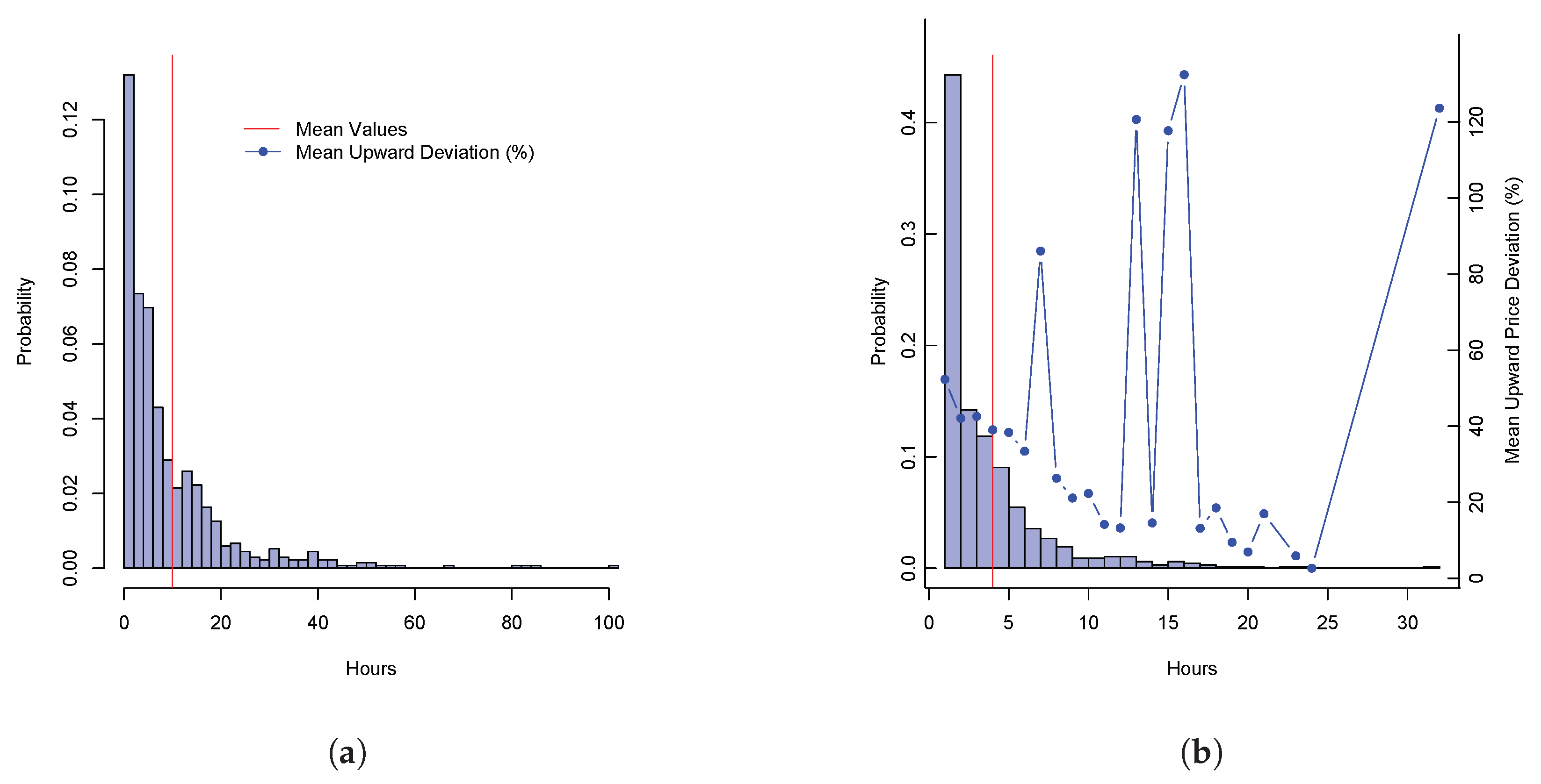
The first step is to gather previous observations from the balancing market to determine the experimental distribution of the duration (time elapsed) in between two upward regulation periods or downward regulation periods, respectively, and the corresponding mean values and . An example for upward regulation is given in Figure 2a, where the red line represents the mean value. In addition, the distribution of the actual duration for each upward and downward regulation period is also obtained (see Figure 2b for upward regulation) along with the mean duration and . At the same time, the observed deviations between day-ahead and balancing market prices are averaged for each duration of regulation (see the function in Figure 2b). By connecting those mean duration values, we get the functions and telling us for each duration of regulation the deviation from the day-ahead market price for upward and downward regulation prices, respectively.
Once the experimental distribution and values for , , , , and are obtained, the scenario generation is started. As in [29], we assume that , , and can be characterized as random variables that follow an exponential distribution, which is a reasonable assumption confirmed by the observations shown in Figure 2. Therefore, random samples of these values can be obtained by applying Equation (8), where and are uniformly distributed variables between zero and one.
The algorithm to generate with a time horizon of periods is summarized in Algorithm 1 and works as follows. For each scenario, we move through the forecasting horizon starting at Period 1. The time to the next regulation period and the duration of this period are sampled based on Equation (8), respectively (Lines 4–5). Based on our current time t and the time to the next period, we can calculate the beginning of the next regulation period (Line 6). The deviations up until are set to zero (Lines 8–10). Starting from period for periods up to , the deviations are set based on the average function and a random error term (Lines 11–13). Next, the current time is updated to (Line 14). In this way, we move through the time horizon until we reach the end . The process is repeated for each scenario and once for upward and once for downward regulation scenarios.
| Algorithm 1 Generate balancing price scenarios. |
| 1: for each do |
| 2: |
| 3: while do |
| 4: where is random |
| 5: where is random |
| 6: |
| 7: |
| 8: for to do |
| 9: = 0 |
| 10: end for |
| 11: for to do |
| 12: = where is random |
| 13: end for |
| 14: |
| 15: end while |
| 16: end for |
| 17: Return |
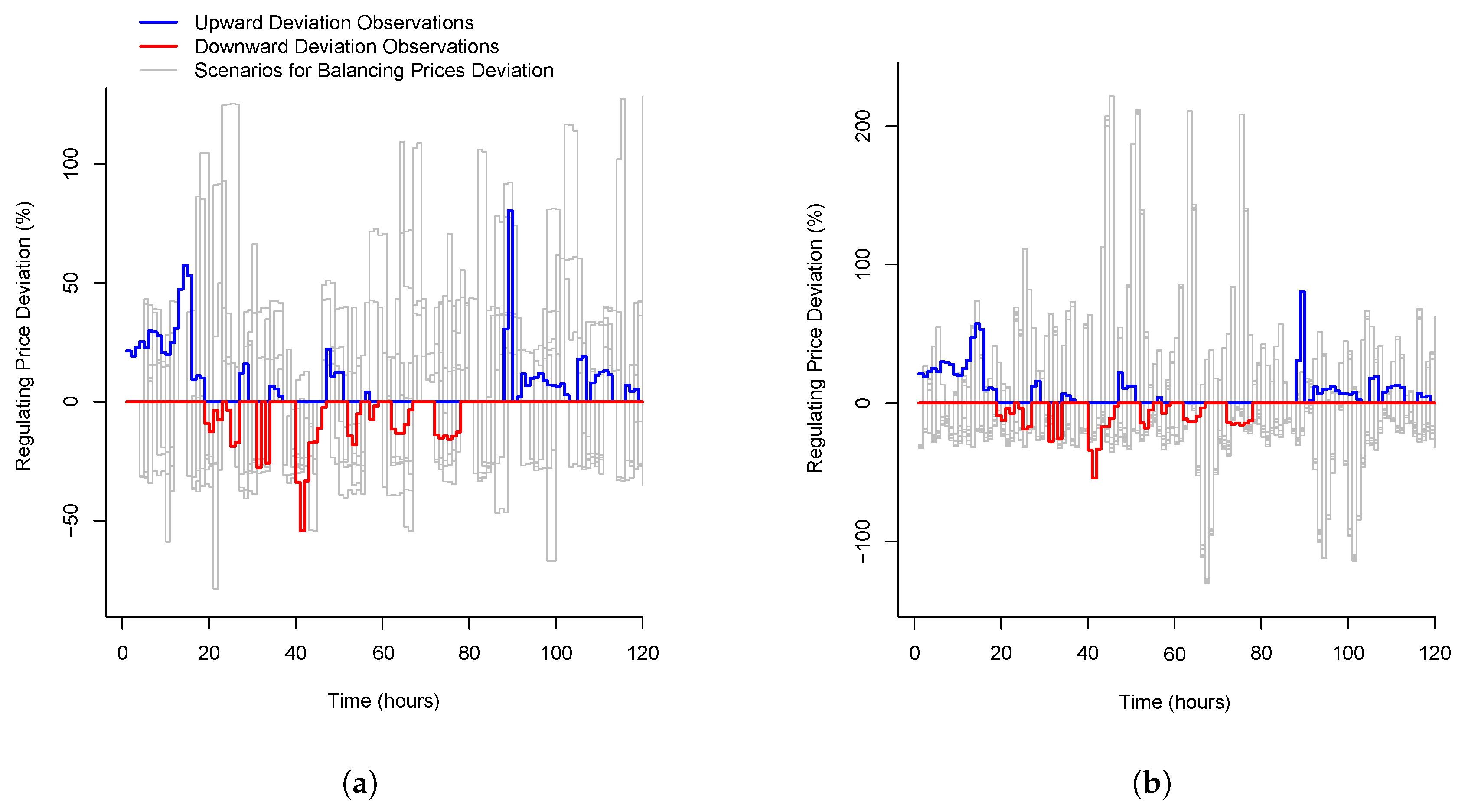
Since upward and downward regulation cannot be activated at the same time, we calculate the final deviation scenario matrix as , where positive values of represent upward regulation and the negative values downward regulation, respectively. Figure 3a shows a set of balancing price scenarios generated by Algorithm 1 compared to the real observations. In comparison to scenarios generated by the method in Figure 3b, we can see the increased variability of regulating prices in the scenarios generated by Algorithm 1. This is due to the fact that the prices are not based on time-series forecasts like in Figure 3b, but on the observed duration for upward and downward regulation periods. To obtain the final prices, the deviation value is multiplied with respective day-ahead market price.
4. Operational Scheduling and Bidding Method
The overall method, which allows the DH operator to schedule the production and determine the bidding curves for the day-ahead and balancing market, uses the two models presented in Section 2 with the scenarios generated by the methods in Section 3. The optimization for one day in practice includes the following steps.
The day before the day in question, the day-ahead market optimization model (3a)–(3c) is solved as two-stage stochastic programming. The model includes scenarios representing the uncertainty regarding day-ahead market electricity prices (Section 3.3), wind power production (Section 3.1) and solar heat production (Section 3.2) for at least 24 h. The scenarios are generated using the Monte Carlo simulation and clustering technique described in Section 3.4. The planning horizon can be considered as longer than 24 h in a rolling horizon manner to include future days in the optimization to get better approximation of the thermal storage behavior, which can store heat longer than just 24 h. The optimal values of the variables in model (3a)–(3c) return the bidding amounts for each hour , while each scenario sets one step in the bidding curve. As constraints (2c) and (2d) ensure the same production amounts for the same electricity prices and increasing production amounts for increasing prices, the optimal values result automatically in a non-decreasing step-wise bidding curve. The bidding prices for each step in the bidding curve are the respective electricity price forecast values .
After the day-ahead market is cleared, the real electricity prices for each hour become available, and the won bids can be determined (i.e., the hours where the bidding price was equal to or below the market price). In hours with won bids, the DH operator is committed to provide the offered amount of power, otherwise the caused imbalance is penalized with a payment. However, imbalances from other operators on the market offer an opportunity for profit. The balancing market is used by the TSO to reduce the imbalances in the system by accepting new bids for additional power or reducing production. Thus, we can use the flexibility in our portfolio of production units to also offer upward and downward regulation bids in the balancing market. As the balancing market has a time horizon of only one hour and is closed shortly before this hour, an optimization needs to take place every hour before the balancing market closes. The model (5a)–(5c) optimizes the production for the next hour taking the committed production from the day-ahead market into account. Furthermore, the model can take several hours into the future into account to anticipate the impact on the remaining hours of the day. The model is again a two-stage stochastic program considering the balancing market price scenarios (see Section 3.5) for all hours and wind power scenarios for later during the day (we assume that the wind power for the next hour can be predicted accurately). Again, the optimal values of and result automatically in non-decreasing or non-increasing step-wise bidding curves representing upward and downward regulation bids, respectively. The bidding prices for each step in the bidding curve are the respective electricity price forecast values and . This step is repeated by the operator for each hour.
5. Case Study
We use the Hvide Sande DH system (see Hvide Sande Fjernvarme A.m.b.A., https://www.hsfv.dk/) in Western Jutland, Denmark, as a case study to evaluate our method. However, the method presented in this paper is applicable to all DH systems with a portfolio of units, because the models in Section 2 are formulated in a general manner and the scenario generation methods Section 3 can be replaced by other available forecasting techniques without changing the overall methodology.
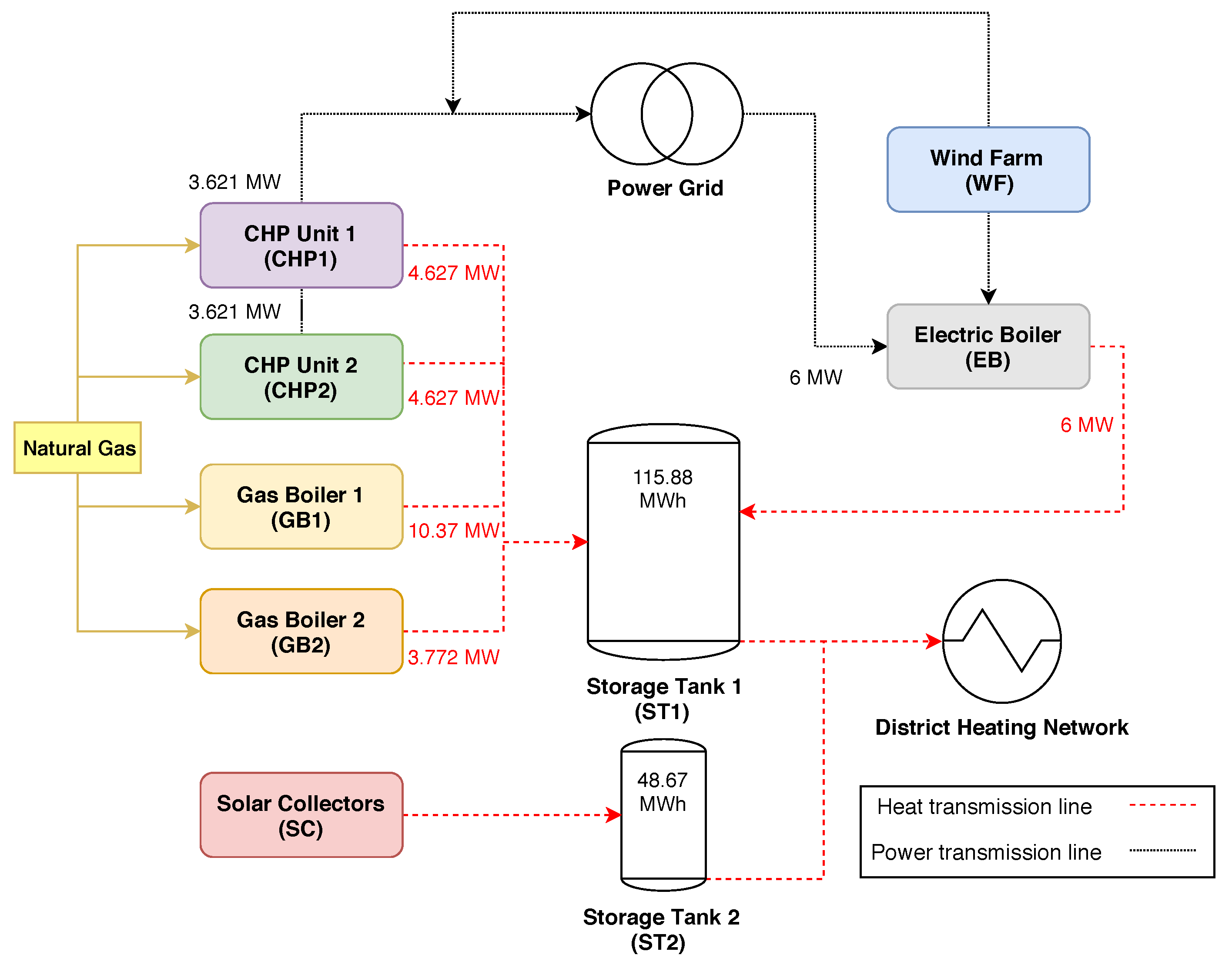
An overview of the Hvide Sande system is given in Figure 4. It has two small gas-fired CHP units (CHP1 and CHP2) acting on the electricity market and feeding heat to the DH system as well as two gas boiler (GB1 and GB2) units with dispatchable heat production. Stochastic renewable heat production comes from a solar collector field (SC), which is considered as one unit. Finally, it is also possible to produce heat from electricity using an electric boiler (EB). The electricity can be bought from the power grid as a regular consumer or using a special tariff. This tariff consists of a tax benefit for operating the electric boiler, in which the amount of power injected by our own wind farm (WF) into the grid is at the same time consumed by the electric boiler. This synchronous operation of both units helps the power system to reduce imbalances and provides inexpensive heat production. The DH system has two thermal storages (ST1 and ST2), where one (ST1) is connected only to the solar collector field and the second storage (ST2) is used by all other units. The parameters for costs and capacities as well as the connections between units are given in Table 3. Furthermore, the table shows to which set the units belong.
6. Analysis of the Experimental Results
To evaluate our approach, we have to determine the real costs and behavior of the system. The actual wind power production, solar thermal production, and heat demand values were obtained from the Hvide Sande DH system for the year 2017. The day-ahead, upward, and downward electricity prices were taken from the Nord Pool market for the bidding area DK1 (where Hvide Sande is located). These data are public and can be downloaded from [32]. The data basis for forecasting and scenario generation was historical data from 15 days before the day in question. The input data for wind speed, solar radiation, and ambient temperature were randomly perturbed values of the real data. The overall evaluation process included the following steps:
- After day-ahead market closure for day d (day ): Evaluate the day-ahead market bids with the now known electricity prices and save production amounts of won bids.
- Each hour on day d:
- (a)
- (b)
- Evaluate the balancing-market bids with the now known balancing electricity prices; fix the committed production amounts; and resolve the model to get actual costs and thermal storage levels.
- Move to the next day
The forecasting and scenario generation were implemented in R 3.2.2, while the optimization models were built in GAMS 24.9.2 using CPLEX 12.1.1 to solve them. All experiments were executed on the DTU HPC Cluster using the 2xIntel Xeon Processor X5550 and 24 GB memory RAM. For the results presented in the remainder of this section, we use a rolling horizon of three days in the day-ahead optimization problem and 12 h for the balancing market problem. To correlate different scenarios of RES with electricity prices, we generate n different scenarios for wind power and solar heat production and m scenarios for electricity prices. The combination of all scenarios results in a total number of scenarios. For the sake of simplicity, we generate scenarios of RES production for the experiments that consider bidding curves.
6.1. Influence of Uncertainty and Number of Bidding Curve Steps on the Day-Ahead Market Results
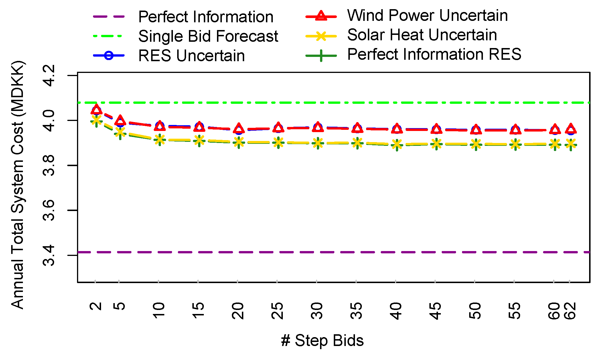
In the first experiment, we concentrated on the bidding results from the day-ahead market optimization problem (3a)–(3c) only. We compared the total annual costs of different setups regarding uncertainty consideration, i.e., which values are known or unknown, and the number of electricity price scenarios resulting in the steps for the bidding curves. The results are given in Figure 5, where the x-axis represents the number of steps in the bidding curve (i.e., the number of electricity price scenarios) and the y-axis represents the total annual system costs. The depicted lines show the results of different setups regarding uncertainty consideration. The theoretically best result was given by considering that we have perfect knowledge about the future electricity prices and RES production (perfect information). However, this value can never be reached in practice due to the uncertainty and, therefore, served only as a benchmark. Another value to compare to is a bidding method that submits bids according to the expected electricity price (single bid forecast), i.e., the model considers no electricity price scenarios, but the expected value resulting in one bidding amount and price for each hour. This approach is often used in practice. The other four approaches consider the model from Section 2.1 to create bidding curves based on uncertain electricity prices. We compared four cases regarding the information about RES production: scenarios for wind power and solar thermal production (RES uncertain), scenarios for wind power and perfect information about solar thermal production (wind power uncertain), scenarios for solar thermal and perfect information about wind power production (solar heat uncertain as well as perfect information regarding both (perfect information RES).
The results from Figure 5 indicate that considering the solar thermal production as uncertain and modeling it as scenarios did not deteriorate the costs significantly compared to the case where the RES production was known. On the other hand, considering the wind power production as uncertainty captured in scenarios had an impact on the costs and led to an increase in the cost of approximately 62,000 DKK (Danish krone). Similar results were achieved when considering both RES production sources as uncertain. Based on these results, we can conclude that especially the uncertainty of the wind power production had an influence on the system costs. This behavior can be explained based on the fact that the wind power production had a direct effect on the power amount that was traded on the electricity market and therefore on the profits obtained. In contrast, the uncertainty of solar thermal production had no large effect due to the thermal storage in the system, which smoothed the effect on the heat production and therefore also the costs. The factor that had the greatest impact on the operational cost is not having information about the day-ahead prices (perfect information). In this case, having perfect information of RES and uncertain day-ahead electricity prices increased the annual system cost by approximately 500,000 DKK (around 12.5% of the total system cost). However, under the real-world condition that RES and electricity prices are uncertain, using stochastic programming to generate bidding curves decreased the cost by ca. 120,000 DKK per year (3% of the total system cost) compared to the single bid forecast.
Figure 5 also shows the influence of the number of steps in the bidding curves. For this experiment the number of clusters in the PAM algorithm was varied (see Section 3.4) to obtain different numbers of scenarios representing the number of steps in the bidding curve. We compared in total 14 scenario set sizes ranging from 2–62 scenarios, which are the minimum and the maximum number of steps allowed to submit to the Nord Pool market [33], respectively. The results show a reduction of costs when the number of steps was increased from two to 20 steps. In this case, including more steps did not lead to further significant reductions in costs.
Based on the analysis in this section, we can conclude that using bidding curves, in particular with at least 20 steps, created from our stochastic program can reduce the annual system cost, in particular compared to single bids based on price forecasts. Furthermore, the uncertainty of wind power production influences the results more than the uncertainty regarding solar thermal production.
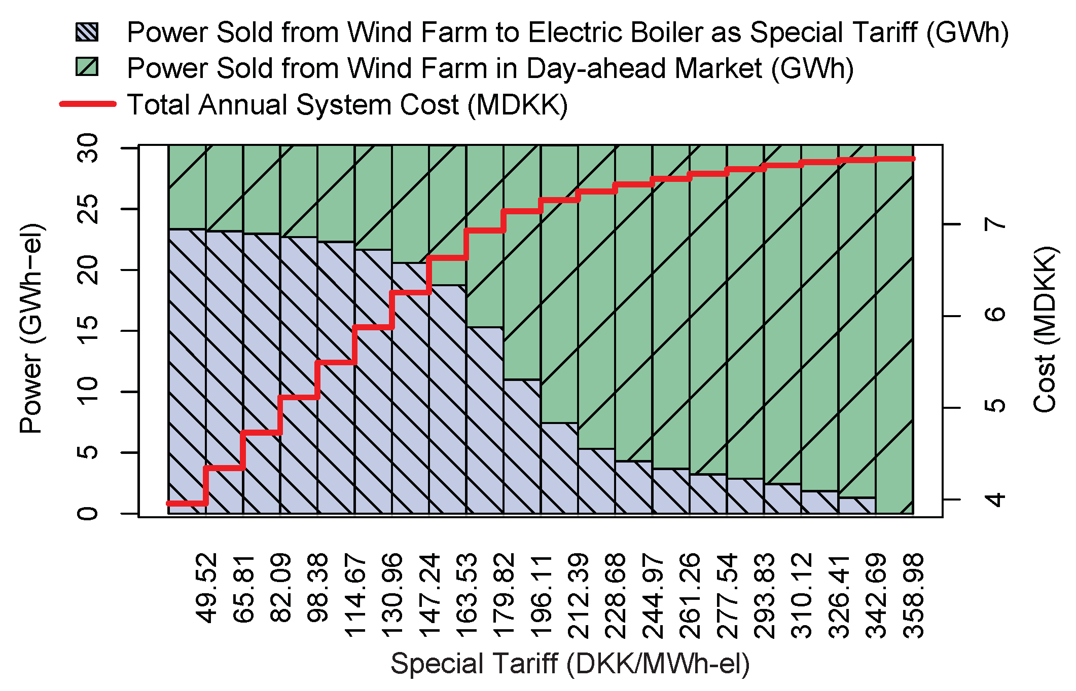
6.2. Impact of Special Tariff for the Electric Boiler
As mentioned in the problem description in Section 2, we assumed a special tariff (in terms of tax reduction) if the electric boiler was “using” power that we provided with our wind farm. In this section, we want to analyze the influence of this tariff on the trading on the day-ahead market. The operational cost under the special tariff was given with 49.52 DKK/MWh-heat. Figure 6 shows the impact on the annual system cost and share of wind power used for the electric boiler and traded on the day-ahead market, respectively, when the tariff was increased in equal step sizes up to the normal operational cost (when fed with power from the grid without a special tariff).
Figure 6 shows clearly the benefits from having a special agreement when feeding in wind power and therefore receiving a special tariff on the electricity consumption. First, the total annual system cost drastically increased when the special tariff became more expensive. This is obvious as the production of heat from electricity was becoming more expensive. Furthermore, it can be seen that the amount of wind power traded on the day-ahead market increased with a higher tariff, because the income from the market was more promising in most of the hours in the year. This means, using the special tariff for the electric boiler is only beneficial if the income from the market is expected to be less than the benefit from using the wind power for the electric boiler. This margin was becoming smaller with increasing special tariff, resulting in higher trade volumes on the day-ahead market.
This results indicate that DH operators can greatly benefit from receiving a special agreement with respect to using our own RES power generation for heat production.
6.3. Analysis of Yearly Production
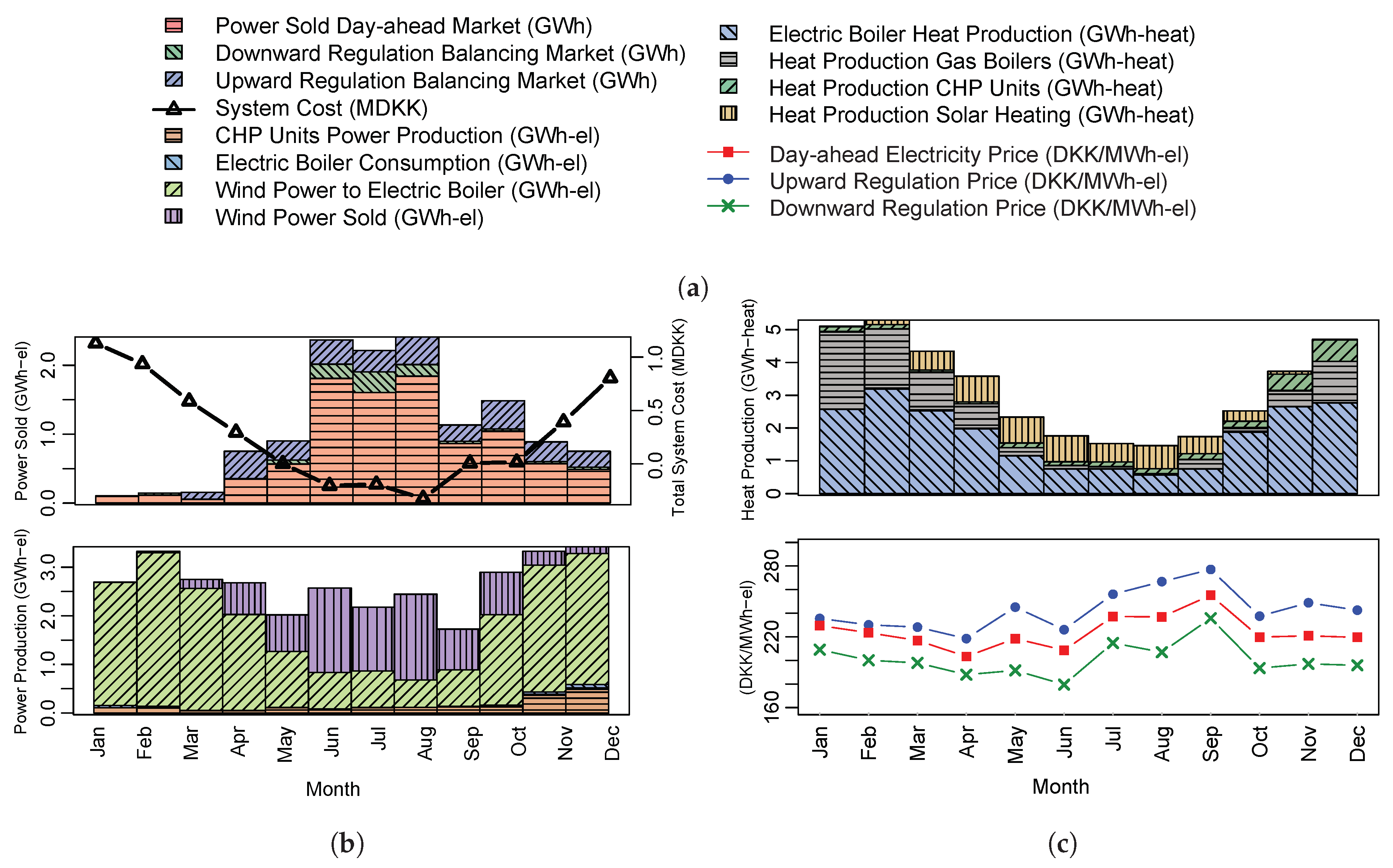
In this section, we provide the results of the annual system behavior when using the solution approach for day-ahead market and balancing market optimization presented in Section 4. The results and values for power production and trading, heat production, and electricity prices are consolidated on a monthly basis in Figure 7. The legend can be found in Figure 7a.
Figure 7b (top) shows the monthly system cost and the amounts of power traded on the day-ahead market as well as down regulation bought and upward regulation sold on the balancing market. One observation from this figure is that the monthly costs were significantly lower during the summer period due to two reasons. First, the amount of power traded on the different electricity markets was higher during the summer, resulting in higher profits. Furthermore, the electricity prices were slightly higher during the summer (see Figure 7c (bottom)). Second, the heat demand was lower during the summer resulting in lower total costs (see Figure 7c (top)). Furthermore, from Figure 7c (top), it can be seen that the solar thermal production was higher during summer, resulting in less heat needed from the more expensive other units.
A second observation is that the trades on the balancing markets have a higher volume during summer and fall. This behavior can be explained by taking the power production on a unit-basis into account, as provided in Figure 7b (bottom). During the summer month, less of the power was used for heat production, because there was a lower heat demand, and therefore available for trading on the electricity markets.
The results show that the optimization method made use of the fact that the units were considered as one portfolio and thereby has a flexibility with respect to the production. The trading and production behavior adjusted itself to the best combination in the different seasons to get the lowest heat production costs and highest incomes from the markets. The specific daily system behavior in the case of regulation activities is further analyzed in Section 6.5.
6.4. Value of Including Balancing Market Trading
The next analysis investigates the value of including the balancing market trading into the solution approach. Therefore, we compared two settings: using the solution approach from Section 4 with and without the balancing market optimization. Furthermore, we ran both settings once with perfect information about electricity prices, wind, and solar production and once in a stochastic programming setting with scenarios (as presented in the model formulation in Section 2).
The total annual system cost for those four cases in Table 4 shows that even if we have perfect information about the future, ignoring trading on the balancing market will increase the total system cost immensely, in this case by 37%. This indicates that a high degree of income can be obtained from the balancing market. The results with perfect information are theoretical values, as those cannot be reached in a real-world application due to the uncertainty at the time of planning. This means that when modeling the uncertainty regarding prices and production in a stochastic setting, the system cost naturally increases, here by 7%. However, lower costs were still achieved by including the balancing market as a second step to avoid imbalances and another opportunity for trading. Not considering the balancing market led here to 8% higher system cost for the entire year.
These conclusions are mostly independent of the actual months or seasons, as can be seen from Figure 8. Here, the monthly cost for the four settings followed a similar ranking in each month.
6.5. Behavior of the System in the Case of Upward and Downward Regulation
To further investigate the benefits of trading in the balancing market, we analyze the obtained production schedules for four representative days of the year where upward and downward regulation was offered. Section 6.5.1 and Section 6.5.2 each analyze two specific days in which upward and downward regulation were provided, respectively. The legend used for the production schedule figures in this section is the same as in Figure 7a.
6.5.1. Upward Regulation
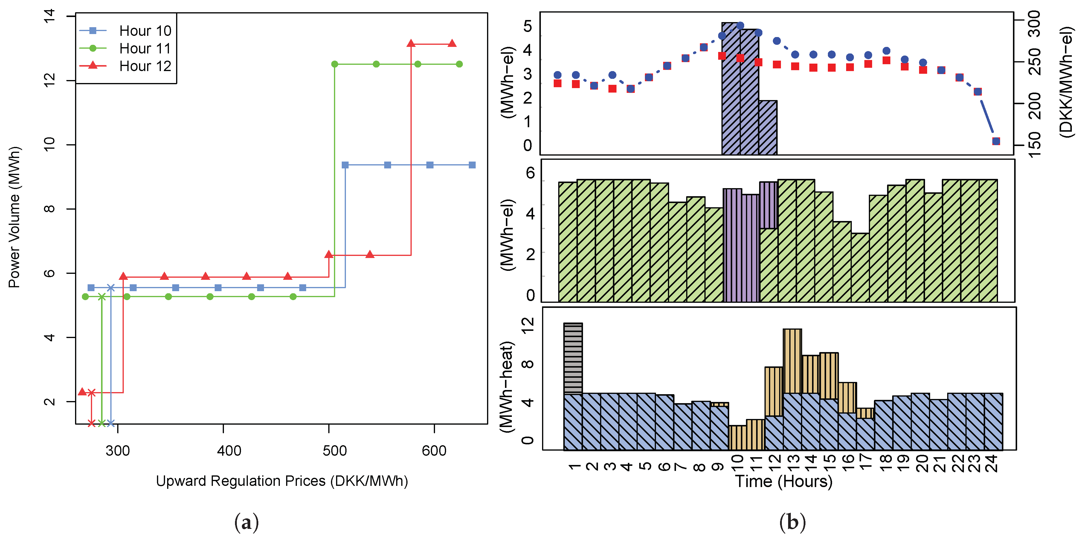
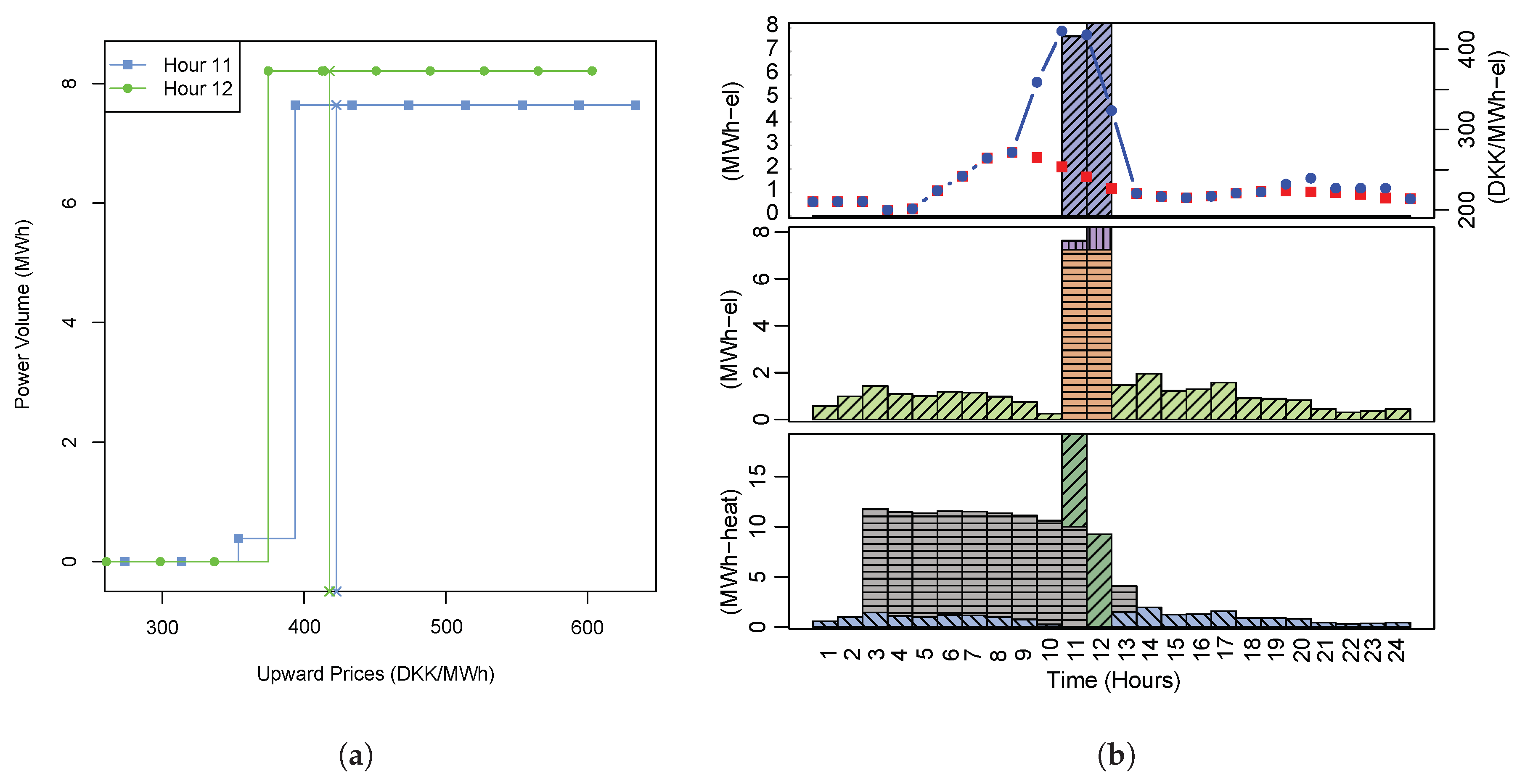
The first case for upward regulation is presented in Figure 9. Figure 9a shows the bidding curves for the hours in which upward regulation was won by the DH operator. The vertical lines delimited with “×” represent the real upward prices for those hours and the corresponding power production offered at such prices. Figure 9b shows the system behavior and is divided into three parts: upward regulation volume per hour including prices (top), hourly power production per unit (middle), and hourly heat production per unit (bottom). As we can see from Figure 9b (middle), the upward regulation in this case is entirely provided by the wind farm. Since no wind power was sold on the day-ahead market, the producer decided to bid the entire production of the wind farm into the balancing market for Hours 10 and 11. In Hour 12, the needed power volume for upward regulation was lower than the actual production from wind. Therefore, the remaining power was used to feed the electric boiler. This behavior was confirmed by the heat production (Figure 9b (bottom)). In Hours 10 and 11, there was no production with the electric boiler but in Hour 12.
The second case for upward regulation is displayed in Figure 10, which follows the same structure as Figure 9. Figure 10a shows that two bids for upward regulation are won. As we can see in Figure 10b (middle), the upward balancing regulation was provided by the wind farm and the two CHP units in our system during these two hours. For these two hours, the upward prices were significantly high, and consequently, it was profitable to turn on the two CHP units.
Based on the system behavior on those two representative days, we can summarize the two cases in which the DH operator can provide upward regulation: first, if we have a higher production of wind power than anticipated and offered in the day-ahead market; second, if the upward regulation price is high enough that it is beneficial to start up the rather expensive CHP units.
6.5.2. Downward Regulation
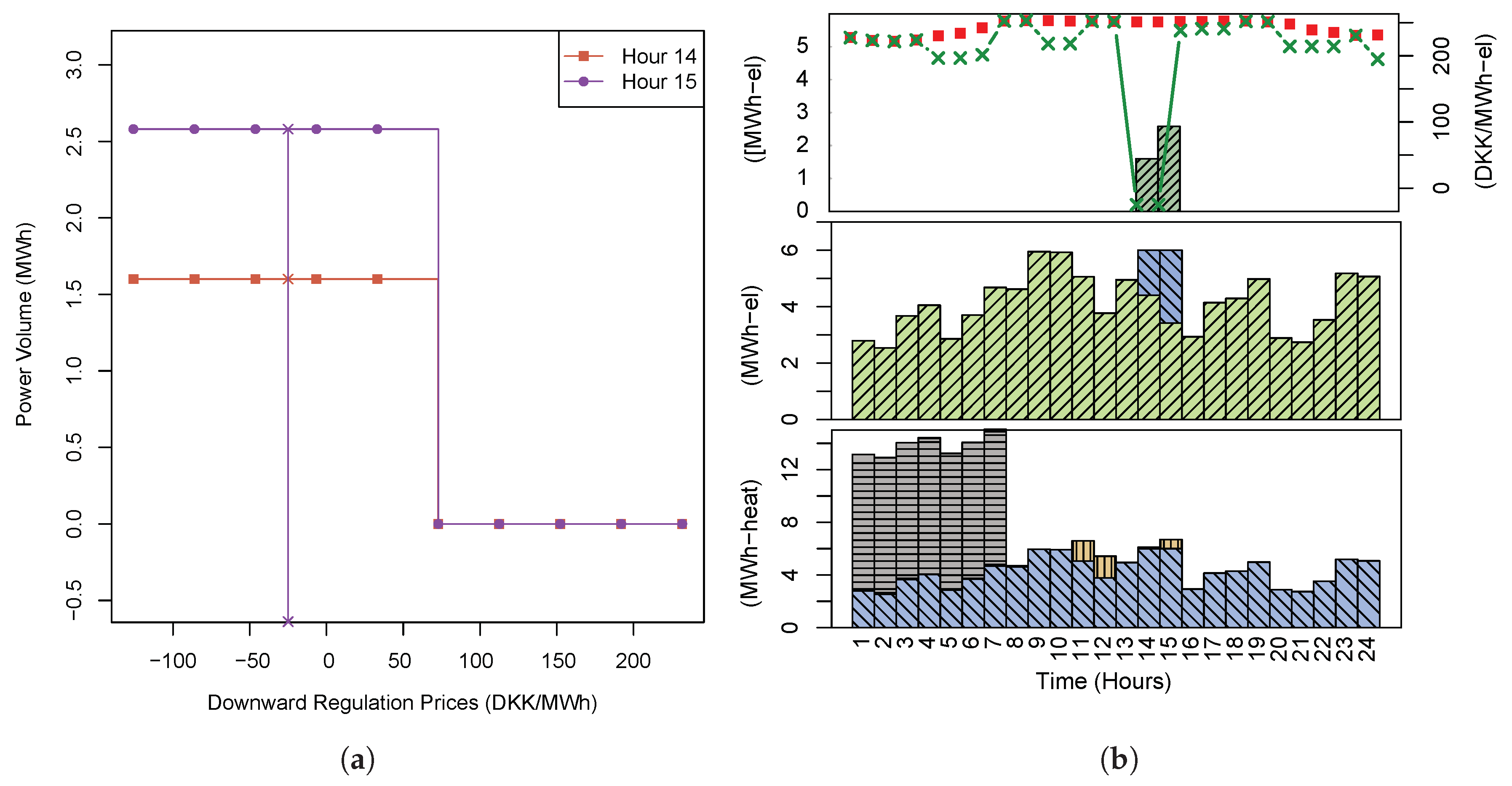
In the following, we analyze how a DH operator can provide downward regulation. The first option is presented in Figure 11, which shows downward regulation provided in Hours 14 and 15. In this case, the model decides to buy electricity from the grid at the downward price and turn on the electric boiler (see Figure 11b (middle). In general, electric boilers are good candidates to provide downward regulation because they can absorb large volumes of power in a very short time. Thus, producing heat using the electric boiler constitutes a very economical option when downward regulation is needed.
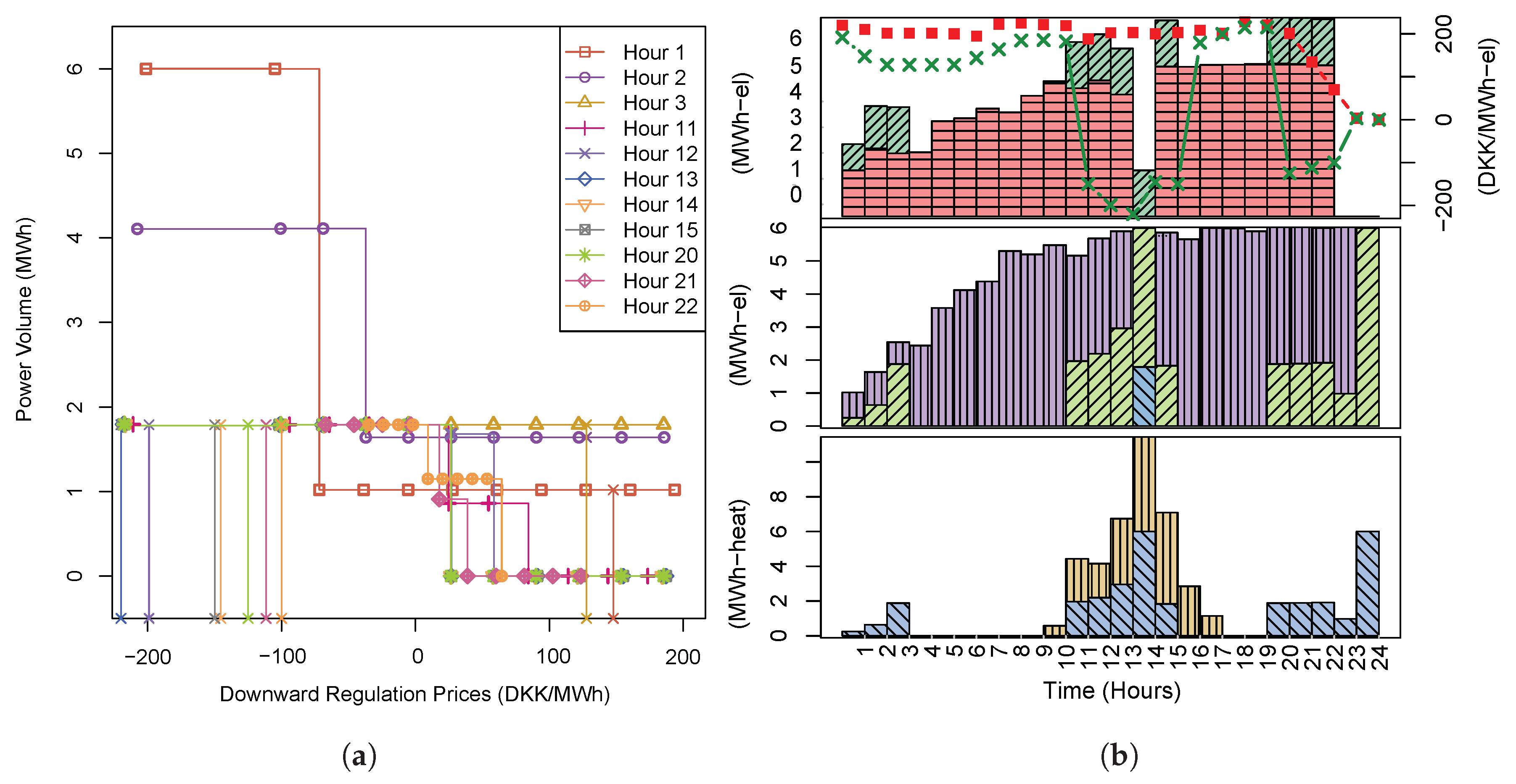
The second option in which our DH system can benefit from downward regulation is shown in Figure 12. In this case, the system took advantage of the power sold previously on the day-ahead market to provide downward regulation. As can be seen from Figure 12a, the system won 11 bids for downward regulation on that specific day. Here, the system stopped providing the day-ahead power previously dispatched and bought this lack of production at the downward price. The profit of the system was the difference between the electricity sold at the day-ahead price and the electricity bought at the balancing price. This behavior is shown in Figure 12b (top), where the difference between the power sold in the day-ahead market and the one sold in the balancing market is the actual production of our wind generators sold to the market (Figure 12b (middle)). This behavior was the same for all time periods where downward regulation was provided with the exception of Hour 14, in which no day-ahead auction was won for that hour, and therefore, the system decided to buy downward regulation and turn on the electric boiler (Figure 12b (middle)).
Based on the results in this section, we can summarize two ways of providing downward regulation for a DH operator. Either the electric boiler is used to provide downward regulation and produce at a low price or previously won power bids on the day-ahead market are corrected due to lower wind power production than excepted.
7. Summary and Outlook
In countries with an extended use of district heating, the integrated operation of DH and power systems can increase the flexibility of the power system, achieving a higher integration of renewable energy sources. However, the operational planning and bidding includes several uncertain components at the time of planning and requires appropriate planning methods. Therefore, we present a planning method based on two-stage stochastic programming that allows DH providers, which operate a portfolio of units and have uncertain RES production, to create price-dependent bids for both day-ahead and balancing markets and optimize the daily production. First, a stochastic program is solved to obtain and present the bids to the day-ahead market. Once the market is cleared, and the producer knows the power production plan, a second stochastic program is used on an hourly basis to generate bids for the balancing market considering the day-ahead power previously dispatched. After the bids for the balancing market are created and submitted, the market is cleared, and the model optimizes the heat production for the new power commitment plan. In addition, we propose a new methodology to define balancing price scenarios that account for the volatility of these latter based on observed mean duration and values.
We perform an extensive analysis of the production and trading behavior of a real DH system in the two markets. The results confirm that uncertain electricity prices have a large impact on the system cost followed by uncertainty in the wind power production. In contrast, solar thermal production uncertainty has a minor influence due to the flexibility given by the heat tank storage. We also show the benefits of using a special tariff that utilizes the power production of wind farms with an electric boiler. This special tariff reduces the yearly total system cost enormously. Regarding the inclusion of balancing market trading into the solution approach, we show that the participation in this market translates into larger profits, resulting in lower operational costs. Finally, we investigate the behavior of the system in the case of upward and downward regulation in more detail. The results emphasize the important role of an electric boiler as a flexible unit connected to the markets. To summarize, we propose a new planning method to reduce the impact of uncertainties on the production planning for DH systems. To the best of our knowledge, no planning and bidding method for DH systems including RES production participating in sequential electricity markets existed before in the literature. We hedge against uncertain electricity market prices and production using stochastic programming to create price-dependent bids. The integration of RES production is facilitated by re-dispatching the imbalances in the balancing market. Furthermore, we show that considering the DH system as the portfolio of units enables the necessary flexibility to react to seasonal changes and uncertainties.
We envision three different lines of future work. The first is to use the presented approach to aggregate offers from a portfolio of different DH producers and calculate the optimally-combined offer that can maximize the profit of all producers considering that we are now price-makers instead of price-takers. Therefore, a bi-level optimization program should be formulated. Second is to improve the bidding strategies to hedge even more against uncertain electricity prices. Finally, our results indicate a significant margin of improvement by using the balancing market. Therefore, it becomes essential to develop more accurate forecasting techniques to predict balancing prices and their high volatility for one or two hours in advance.
Author Contributions
Conceptualization, I.B., D.G. and A.N.A.; formal analysis, I.B.; funding acquisition, H.M.; investigation, I.B. and D.G.; methodology, I.B. and D.G.; project administration, D.G. and H.M.; software, I.B.; supervision, D.G. and H.M.; validation, I.B. and D.G.; writing, original draft, I.B. and D.G.; writing, review and editing, A.N.A.
Funding
This work is partly funded by Innovation Fund Denmark through the CITIES research center (No. 1035-00027B).
Acknowledgments
We would like to thank Hvide Sande Fjernvarme A.m.b.A., especially Martin Halkjær Kristensen, for the valuable input and dataset.
Conflicts of Interest
The authors declare no conflict of interest.
References
- European Commission. Efficient District Heating and Cooling Systems in the EU. 2016. Available online: https://www.euroheat.org/wp-content/uploads/2017/01/study-on-efficient-dhc-systems-in-the-eu-dec2016_final-public-report6.pdf (accessed on 2 February 2018).
- Connolly, D.; Lund, H.; Mathiesen, B.; Werner, S.; Möller, B.; Persson, U.; Boermans, T.; Trier, D.; Østergaard, P.; Nielsen, S. Heat Roadmap Europe: Combining district heating with heat savings to decarbonise the EU energy system. Energy Policy 2014, 65, 475–489. [Google Scholar] [CrossRef]
- Euroheat & Power. District Energy in Denmark. 2017. Available online: https://www.euroheat.org/knowledge-centre/district-energy-denmark/ (accessed on 15 March 2018).
- Danish Energy Agency. Regulation and Planning of District Heating in Denmark. Available online: https://ens.dk/sites/ens.dk/files/Globalcooperation/regulation_and_planning_of_district_heating_in_denmark.pdf (accessed on 10 September 2018).
- Madsen, H.; Parvizi, J.; Sempreviva, A.M.; Bindner, H.W.; Dent, C.; Mackensen, R. Integrated energy systems; aggregation, forecasting, and control. In DTU International Energy Report 2015; Technical University of Denmark (DTU): Kgs. Lyngby, Denmark, 2015; pp. 34–40. [Google Scholar]
- Pezzutto, S.; Grilli, G.; Zambotti, S.; Dunjic, S. Forecasting Electricity Market Price for End Users in EU28 until 2020—Main Factors of Influence. Energies 2018, 11, 1460. [Google Scholar] [CrossRef]
- Kavvadias, K. Energy price spread as a driving force for combined generation investments: A view on Europe. Energy 2016, 115, 1632–1639. [Google Scholar] [CrossRef]
- Pandžić, H.; Morales, J.M.; Conejo, A.J.; Kuzle, I. Offering model for a virtual power plant based on stochastic programming. Appl. Energy 2013, 105, 282–292. [Google Scholar] [CrossRef]
- Carpaneto, E.; Lazzeroni, P.; Repetto, M. Optimal integration of solar energy in a district heating network. Renew. Energy 2015, 75, 714–721. [Google Scholar] [CrossRef]
- Wang, H.; Yin, W.; Abdollahi, E.; Lahdelma, R.; Jiao, W. Modelling and optimization of CHP based district heating system with renewable energy production and energy storage. Appl. Energy 2015, 159, 401–421. [Google Scholar] [CrossRef]
- Li, J.; Fang, J.; Zeng, Q.; Chen, Z. Optimal operation of the integrated electrical and heating systems to accommodate the intermittent renewable sources. Appl. Energy 2016, 167, 244–254. [Google Scholar] [CrossRef]
- Paraschiv, F.; Erni, D.; Pietsch, R. The impact of renewable energies on EEX day-ahead electricity prices. Energy Policy 2014, 73, 196–210. [Google Scholar] [CrossRef] [Green Version]
- Kwon, R.H.; Frances, D. Optimization-Based Bidding in Day-Ahead Electricity Auction Markets: A Review of Models for Power Producers. In Handbook of Networks in Power Systems I; Sorokin, A., Rebennack, S., Pardalos, P.M., Iliadis, N.A., Pereira, M.V.F., Eds.; Springer: Berlin/Heidelberg, Germany, 2012; pp. 41–59. [Google Scholar] [CrossRef]
- Birge, J.R.; Louveaux, F. Introduction to Stochastic Programming; Springer Science & Business Media: New York, NY, USA, 2011. [Google Scholar]
- Schulz, K.; Hechenrieder, B.; Werners, B. Optimal Operation of a CHP Plant for the Energy Balancing Market. In Operations Research Proceedings 2014; Springer International Publishing: Basel, Switzerland, 2016; pp. 531–537. [Google Scholar]
- Ravn, H.V.; Riisom, J.; Schaumburg-Müller, C.; Straarup, S.N. Modelling Danish local CHP on market conditions. In Proceedings of the 6th IAEE European Conference: Modelling in Energy Economics and Policy, Zürick, Switzerland, 2–3 September 2004. [Google Scholar]
- Dimoulkas, I.; Amelin, M. Constructing bidding curves for a CHP producer in day-ahead electricity markets. In Proceedings of the 2014 IEEE International Energy Conference (ENERGYCON), Dubrovnic, Croatia, 13–16 May 2014; pp. 487–494. [Google Scholar]
- Ayón, X.; Moreno, M.Á.; Usaola, J. Aggregators’ Optimal Bidding Strategy in Sequential Day-Ahead and Intraday Electricity Spot Markets. Energies 2017, 10, 450. [Google Scholar] [CrossRef]
- Plazas, M.A.; Conejo, A.J.; Prieto, F.J. Multimarket optimal bidding for a power producer. IEEE Trans. Power Syst. 2005, 20, 2041–2050. [Google Scholar] [CrossRef]
- Pei, W.; Du, Y.; Deng, W.; Sheng, K.; Xiao, H.; Qu, H. Optimal bidding strategy and intramarket mechanism of microgrid aggregator in real-time balancing market. IEEE Trans. Ind. Inf. 2016, 12, 587–596. [Google Scholar] [CrossRef]
- Hosseini-Firouz, M. Optimal offering strategy considering the risk management for wind power producers in electricity market. Int. J. Electr. Power Energy Syst. 2013, 49, 359–368. [Google Scholar] [CrossRef]
- Vardanyan, Y.; Hesamzadeh, M.R. The coordinated bidding of a hydropower producer in three-settlement markets with time-dependent risk measure. Electr. Power Syst. Res. 2017, 151, 40–58. [Google Scholar] [CrossRef]
- Kumbartzky, N.; Schacht, M.; Schulz, K.; Werners, B. Optimal operation of a CHP plant participating in the German electricity balancing and day-ahead spot market. Eur. J. Oper. Res. 2017, 261, 390–404. [Google Scholar] [CrossRef]
- Petrichenko, R.; Baltputnis, K.; Sauhats, A.; Sobolevsky, D. District heating demand short-term forecasting. In Proceedings of the 2017 IEEE International Conference on Environment and Electrical Engineering and 2017 IEEE Industrial and Commercial Power Systems Europe (EEEIC/I&CPS Europe), Milan, Italy, 6–9 June 2017; pp. 1–5. [Google Scholar]
- Pinson, P.; Nielsen, H.A.; Madsen, H.; Nielsen, T.S. Local linear regression with adaptive orthogonal fitting for the wind power application. Stat. Comput. 2008, 18, 59–71. [Google Scholar] [CrossRef] [Green Version]
- EMD International A/S. Solar Collectors and Photovoltaics in Energy PRO. Available online: https://www.emd.dk/files/energypro/HowToGuides/Solar%20collectors%20and%20photovoltaics%20in%20energyPRO.pdf (accessed on 5 September 2018).
- Gonzalez, V.; Contreras, J.; Bunn, D.W. Forecasting power prices using a hybrid fundamental-econometric model. IEEE Trans. Power Syst. 2012, 27, 363–372. [Google Scholar] [CrossRef]
- Ringwood, J.; Austin, P.C.; Monteith, W. Forecasting weekly electricity consumption: A case study. Energy Econ. 1993, 15, 285–296. [Google Scholar] [CrossRef]
- Conejo, A.J.; Carrión, M.; Morales, J.M. Decision Making under Uncertainty in Electricity Markets; Springer Science & Business Media: New York, NY, USA, 2010; Volume 1. [Google Scholar]
- Reynolds, A.P.; Richards, G.; de la Iglesia, B.; Rayward-Smith, V.J. Clustering rules: A comparison of partitioning and hierarchical clustering algorithms. J. Math. Model. Algorithms 2006, 5, 475–504. [Google Scholar] [CrossRef]
- Olsson, M.; Soder, L. Modeling real-time balancing power market prices using combined SARIMA and Markov processes. IEEE Trans. Power Syst. 2008, 23, 443–450. [Google Scholar] [CrossRef]
- Energinet—Energy Data Service. Available online: https://www.energidataservice.dk/en/ (accessed on 3 October 2018).
- Nord Pool Spot Glossary. Available online: https://www.energiforetagen.se/globalassets/energiforetagen/det-erbjuder-vi/kurser-och-konferenser/krisutbildningar/nord-pool-spot-glossary.pdf (accessed on 3 October 2018).
Figure 1.
Wind power prediction process. (a) Wind power curve using real data for one year of power production and wind speed in Nord Pool DK1; (b) wind power predictions for a one-day receding horizon and the normalized wind speed.
Figure 1.
Wind power prediction process. (a) Wind power curve using real data for one year of power production and wind speed in Nord Pool DK1; (b) wind power predictions for a one-day receding horizon and the normalized wind speed.

Figure 2.
Distributions of elapsed time between and duration of upward regulation, as well as average regulating prices for year 2017 in the Nord Pool bidding area DK1. (a) Time elapsed between upward regulation periods; (b) duration of upward regulation and price deviation.
Figure 2.
Distributions of elapsed time between and duration of upward regulation, as well as average regulating prices for year 2017 in the Nord Pool bidding area DK1. (a) Time elapsed between upward regulation periods; (b) duration of upward regulation and price deviation.

Figure 3.
Scenarios for balancing prices. (a) Ten scenarios generated by Algorithm 1; (b) Ten scenarios generated by the method proposed in [31].
Figure 3.
Scenarios for balancing prices. (a) Ten scenarios generated by Algorithm 1; (b) Ten scenarios generated by the method proposed in [31].

Figure 4.
Flowchart of the Hvide Sande district heating system.

Figure 5.
Comparison of different uncertainty setups and number of steps in the bidding curves in the day-ahead market optimization. The values shown are total annual system cost.
Figure 5.
Comparison of different uncertainty setups and number of steps in the bidding curves in the day-ahead market optimization. The values shown are total annual system cost.

Figure 6.
Power from the wind turbines used for the electric boiler as a special tariff or traded on the day-ahead market as well as total annual system cost. The values are given for varying the special tariff operation cost of the electric boiler.
Figure 6.
Power from the wind turbines used for the electric boiler as a special tariff or traded on the day-ahead market as well as total annual system cost. The values are given for varying the special tariff operation cost of the electric boiler.

Figure 7.
Annual system behavior on a monthly time-scale. (a) Legend; (b) power sold on the markets and system cost (top), as well as power production by the different units (bottom); (c) heat production by the different units (top) and average electricity prices (bottom).
Figure 7.
Annual system behavior on a monthly time-scale. (a) Legend; (b) power sold on the markets and system cost (top), as well as power production by the different units (bottom); (c) heat production by the different units (top) and average electricity prices (bottom).

Figure 8.
Comparison of monthly system cost in different setups of the solution approach.

Figure 9.
Upward regulation provided on 9 March 2017. (a) Bidding curves and won bids (marked with ×); (b) system operation: upward regulation amount including day-ahead and balancing prices (top), power production (middle), and heat production (bottom).
Figure 9.
Upward regulation provided on 9 March 2017. (a) Bidding curves and won bids (marked with ×); (b) system operation: upward regulation amount including day-ahead and balancing prices (top), power production (middle), and heat production (bottom).

Figure 10.
Upward regulation provided on 27 March 2017. (a) Bidding curves and won bids (marked with ×); (b) system operation: upward regulation amount including day-ahead and balancing prices (top), power production (middle), and heat production (bottom).
Figure 10.
Upward regulation provided on 27 March 2017. (a) Bidding curves and won bids (marked with ×); (b) system operation: upward regulation amount including day-ahead and balancing prices (top), power production (middle), and heat production (bottom).

Figure 11.
Downward regulation provided on 6 February 2017. (a) Bidding curves and won bids (marked with ×); (b) system operation: day-ahead committed amount, downward regulation amount, as well as day-ahead and balancing prices (top), power production (middle), and heat production (bottom).
Figure 11.
Downward regulation provided on 6 February 2017. (a) Bidding curves and won bids (marked with ×); (b) system operation: day-ahead committed amount, downward regulation amount, as well as day-ahead and balancing prices (top), power production (middle), and heat production (bottom).

Figure 12.
Downward regulation provided on 10 September 2017. (a) Bidding curves and won bids (marked with ×); (b) system operation: day-ahead committed amount, downward regulation amount, as well as day-ahead and balancing prices (top), power production (middle), and heat production (bottom).
Figure 12.
Downward regulation provided on 10 September 2017. (a) Bidding curves and won bids (marked with ×); (b) system operation: day-ahead committed amount, downward regulation amount, as well as day-ahead and balancing prices (top), power production (middle), and heat production (bottom).


Table 1.
Nomenclature (DKK = Danish krone).
| Sets | |
| Set of time periods t | |
| Set of heat production units u | |
| Subset of CHP production units | |
| Subset of heat-only production units | |
| Subset of power to heat production units | |
| Subset of stochastic heat production units | |
| Set of intermittent renewable power-only producers g | |
| Set of heat storage tanks s | |
| Set of scenarios | |
| Parameters | |
| Cost for producing heat with unit (DKK/MWh-heat) | |
| Tariff cost for producing power with unit and using it to produce heat in unit (DKK/MWh-el) | |
| Maximum/minimum heat production for unit (MWh-heat) | |
| Binary parameter: 1, if unit is connected to the DH system, 0 otherwise | |
| Binary parameter: 1, if unit is connected to the thermal storage s, 0 otherwise | |
| Heat-to-power ratio for unit () | |
| Initial level in storage s (MWh-heat) | |
| Maximum/minimum heat level in storage s (MWh-heat) | |
| Electricity price for time period (DKK/MWh-el) | |
| / | Penalty for positive/negative imbalance in time period (DKK/MWh-el) |
| / | Upward/downward regulating price for time period (DKK/MWh-el) |
| Heat demand for time period (MWh-heat) | |
| Stochastic power production of power-only unit | |
| Stochastic heat production from heat production unit | |
| Probability of scenario | |
| Parameter that determines the deviation of the penalty for the positive and negative imbalance | |
| Variables | |
| Power bid to the day-ahead market unit in period (MWh-el) | |
| Heat production of heat unit in period (MWh-heat) | |
| Heat production of unit inserted into the grid in period (MWh-heat) | |
| Heat production of unit inserted into storage s in period (MWh-heat) | |
| Power production of unit in period (MWh-el) | |
| Power obtained from the grid to produce heat with unit in period (MWh-el) | |
| Power production of unit that serves the heat production of unit in period (MWh-el) | |
| Power generation from unit in period (MWh-el) | |
| Positive/negative power imbalance purchased/sold in period and scenario (MWh-el) | |
| Upward/downward regulating power purchased/sold in period and scenario (MWh-el) | |
| Level in storage s at time period (MWh-heat) | |
| Heat flowing from the storage s to the DH in period (MWh-heat) | |
Table 2.
Nomenclature for balancing price scenario generation.
| Mean time to activate upward regulation (hours) | |
| Mean time to activate downward regulation (hours) | |
| Mean duration for upward regulation (hours) | |
| Mean duration for downward regulation (hours) | |
| Function for the upward regulation value given an upward time duration length | |
| Function for the downward regulation value given a downward time duration length | |
| Matrix of values for the upward regulation (%) | |
| Matrix of values for the downward regulation (%) | |
| Number of considered scenarios | |
| Forecast horizon | |
| Random variables uniformly distributed between 0 and 1 | |
| Normally-distributed random noise added to the function / |
Table 3.
Characteristics of the production units and thermal storages.
| Unit | Set | ||||||||
|---|---|---|---|---|---|---|---|---|---|
| ST1 | ST2 | ||||||||
| CHP1 | 689.01 | - | 4.63 | 3.62 | 1.28 | 0 | 1 | 0 | |
| CHP2 | 689.01 | - | 4.63 | 3.62 | 1.28 | 0 | 1 | 0 | |
| GB1 | 401.30 | - | 10.37 | 0.00 | - | 0 | 1 | 0 | |
| GB2 | 416.29 | - | 3.77 | 0.00 | - | 0 | 1 | 0 | |
| EB | 359.98 | 49.52 | 6.00 | 0.00 | 1.00 | 0 | 1 | 0 | |
| SC | 0.00 | - | 100.00 | 0.00 | - | 0 | 0 | 1 | |
| WF | 0.00 | - | 0.00 | 0.00 | - | - | - | - | |
| ST1 | 115.88 | 0.00 | 57.94 | ||||||
| ST2 | 48.67 | 0.00 | 24.34 | ||||||
Table 4.
Comparison of the annual system cost in different setups of the solution approach.
| Setting | Total System Cost (DKK) | |
|---|---|---|
| Perfect information incl.balancing market | 2,499,205 | - |
| Perfect information excl.balancing market | 3,414,310 | +37% |
| Stochastic incl. balancing market | 3,655,798 | +7% |
| Stochastic excl. balancing market | 3,956,530 | +8% |
© 2018 by the authors. Licensee MDPI, Basel, Switzerland. This article is an open access article distributed under the terms and conditions of the Creative Commons Attribution (CC BY) license (http://creativecommons.org/licenses/by/4.0/).
Share and Cite
MDPI and ACS Style
Blanco, I.; Guericke, D.; Andersen, A.N.; Madsen, H. Operational Planning and Bidding for District Heating Systems with Uncertain Renewable Energy Production. Energies 2018, 11, 3310. https://doi.org/10.3390/en11123310
AMA Style
Blanco I, Guericke D, Andersen AN, Madsen H. Operational Planning and Bidding for District Heating Systems with Uncertain Renewable Energy Production. Energies. 2018; 11(12):3310. https://doi.org/10.3390/en11123310
Chicago/Turabian StyleBlanco, Ignacio, Daniela Guericke, Anders N. Andersen, and Henrik Madsen. 2018. "Operational Planning and Bidding for District Heating Systems with Uncertain Renewable Energy Production" Energies 11, no. 12: 3310. https://doi.org/10.3390/en11123310
Note that from the first issue of 2016, this journal uses article numbers instead of page numbers. See further details here.