A University Building Test Case for Occupancy-Based Building Automation

Abstract

Heating, ventilation and air-conditioning (HVAC) units in buildings form a system-of-subsystems entity that must be accurately integrated and controlled by the building automation system to ensure the occupants’ comfort with reduced energy consumption. As control of HVACs involves a standardized hierarchy of high-level set-point control and low-level Proportional-Integral-Derivative (PID) controls, there is a need for overcoming current control fragmentation without disrupting the standard hierarchy. In this work, we propose a model-based approach to achieve these goals. In particular: the set-point control is based on a predictive HVAC thermal model, and aims at optimizing thermal comfort with reduced energy consumption; the standard low-level PID controllers are auto-tuned based on simulations of the HVAC thermal model, and aims at good tracking of the set points. One benefit of such control structure is that the PID dynamics are included in the predictive optimization: in this way, we are able to account for tracking transients, which are particularly useful if the HVAC is switched on and off depending on occupancy patterns. Experimental and simulation validation via a three-room test case at the Delft University of Technology shows the potential for a high degree of comfort while also reducing energy consumption.

1. Introduction

Heating, Ventilation and Air-Conditioning (HVAC) systems, widely used in residential and commercial buildings, are responsible for a large part of the global energy consumption [1]. According to the European Commission’s Joint Research Center, Institute for Energy (2009), HVAC systems in the European Union member states were estimated to account for approximately 313 TWh of electricity use in 2007, about $11\%$ of the total 2800 TWh consumed in Europe that year [2]. Energy savings in HVAC systems were therefore identified as a key element to fulfill the target of reducing energy consumption by $20\%$ by 2020. Increased attention has been focused on the reduction of HVAC energy consumption (without violating comfort requirements) [3], via more efficient equipment [4,5,6], novel approaches to HVAC energy storage [7] or supervisory control techniques [8,9,10]. A recent literature review of control methods, with an emphasis on the theory and applications of model predictive control for HVAC systems can be found in [11].

Typical HVAC systems are comprised of boilers, air handling units (AHUs), Variable Air Volume (VAV) boxes, radiators, thermal zones, valves, dampers, fans, pumps, pipes and ducts. The primary drawback with the current state of the art is that separate control systems are designed for each HVAC component, where the design is carried out to ensure that a certain constant reference set point is maintained. Integrating all of these single components require a tedious manual effort by HVAC system installers to tune all these set points: apart from the enormous tuning effort [12], it is difficult to explicitly account for changing conditions, e.g., individual comfort of occupants or their occupancy patterns. Very often, thermal discomfort often leads to constant correction of temperature set-points by the users, causing increased energy consumption [13,14]. Thus, it is necessary to develop a model-based approach with the ability to integrate the human thermal comfort along with various HVAC components. However, as thermal comfort of the users is season-dependent and highly subjective, there exist various attempts to quantify it according to the physical characteristics of both the occupants and their surroundings. Widely-used thermal comfort models are the Adaptive Comfort Model [15] and the Predicted Mean Vote (PMV) [16], where the latter is considered in this work because it is most suited in the absence of natural ventilation. Recent works on occupancy-based building indoor climate control, also touching upon thermal comfort topics, can be found in [17,18].

While there exist many intelligent HVAC control algorithms, they often require the deployment of a completely new control architecture. On the other hand, control architecture for building automation is quite standardized: in particular, most HVAC low-level controllers commissioned in the field today are of Proportional-Integral (PI) or Proportional-Integral-Derivative (PID) type. Therefore, there exists a need to integrate modern controllers with existing PID controllers to ensure that the control objectives are met. Furthermore, current research in Building Management Systems (BMSs) has turned towards Model Predictive Controllers (MPC) for optimal control of building systems, thanks to its capability of handling external disturbances [19], linear and nonlinear models with multiple constraints [20,21]. In view of this situation, in this work, we propose an integrated control structure using an upper MPC layer and lower PID layer. The MPC is based on an integrated HVAC model and generates set-points for the lower layer based on energy and comfort optimization, while the lower level controllers is composed of PI controllers auto-tuned so as to track the reference set-points. One of the main benefits of the integrated control structure is that the PID dynamics can be easily included in the MPC optimization [22]: in this way, we are able to account for tracking transients, which are particularly useful if the HVAC has to be switched on and off depending on occupancy patterns [23]. By doing this, we are able to achieve integration of HVAC and occupants via a PMV index. To the best of our knowledge, the studies available in literature about MPC for office buildings, e.g., [24,25] and references therein, typically neglect such transients. In recent years, there has been a considerable effort in using building energy performance models such as EnergyPlus and TRNSYS [26] not only for simulation and energy consumption purposes, but also for assisting in evaluation of controller design [27,28]. In this work, the proposed control strategy is experimentally validated via an EnergyPlus building energy performance model of a three-room test case at the Delft University of Technology.

This paper will be organized as follows. Section 2 introduces the HVAC test case we consider. Section 3 outlines the optimization problem for both control layers. Section 4 validates the model with real-life data and with EnergyPlus simulations. Section 5 deals with the simulation and results and conclusions are drawn in Section 6. All symbols introduced in the text can be found in Appendix A.

2. Modelling of HVAC Dynamics

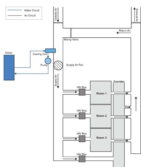
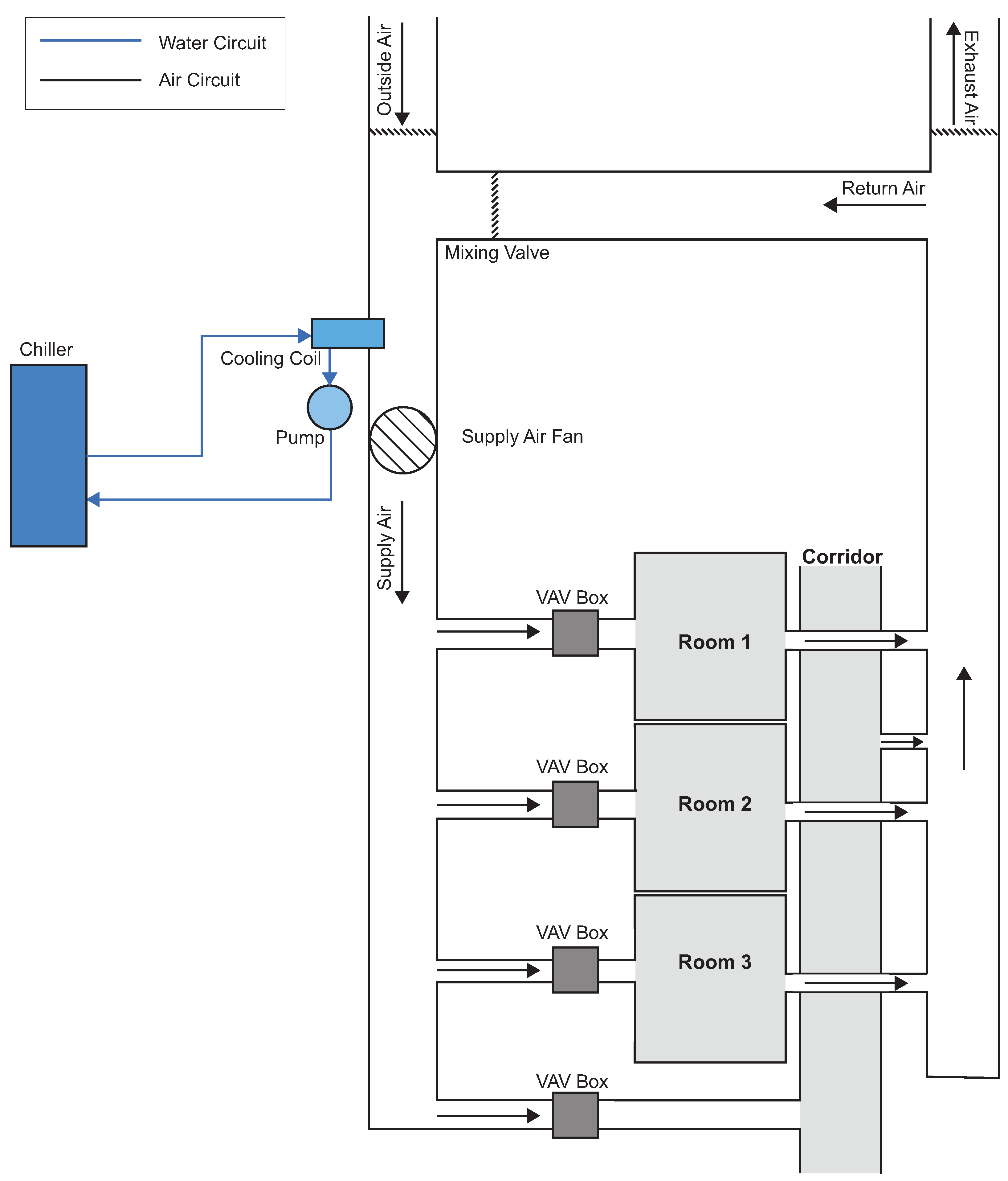
We will focus on the cooling test case shown in Figure 1, which models the dynamical interactions between three rooms and one corridor in the Mechanical Engineering faculty of Delft University of Technology (TU Delft). Figure 1 highlights the multi-component interacting structure of the HVAC system, with a chiller driving a cooling coil of an AHU, with the AHU being further connected to a VAV system which supplies fresh air into the rooms and the corridor. Cold water is supplied with a variable-speed pump to the cooling coil, and the fan in the AHU is a variable-speed fan as well. The three rooms have dimensions 16 m${}^2$, 16 m${}^2$ and 20 m${}^2$, with a corridor of 26 m${}^2$. The chiller has capacity of 2 m${}^3$ and maximum energy of 2 kW. The three rooms are subject to a variable occupancy schedule.

The overall integrated model of the HVAC system is a simplified version of the model developed in [29]. The corresponding dynamics are:

$$\begin{array}{cc}\hfill \left[\mathrm{Chiller}\right]\frac{d{T}_c}{dt}& =\frac{Q_c}{c_w{\rho }_w{V}_c}+\frac{u_w}{{\rho }_w{V}_c}(T_{c_{rw}}-T_c),\hfill \\ \hfill \left[\mathrm{Cooling}\mathrm{coil}\right]\frac{d{T}_{cc}}{dt}& =\frac{u_w}{{\rho }_w{V}_p}(T_c-T_{cc})+\frac{h_{cc}{A}_{cc}}{c_w{\rho }_w{V}_p}(T_s-T_c),\hfill \\ \hfill \left[\mathrm{AHU}\right]\frac{d{T}_s}{dt}& =\frac{u_a}{{\rho }_a{V}_d}(u_d{T}_{rm}+(1-u_d)T_{out}-T_{ma})\hfill \\ & +\frac{h_{cc}{A}_{cc}}{c_a{\rho }_a{V}_d}(T_s-T_{cc}).\hfill \end{array}$$

(1)

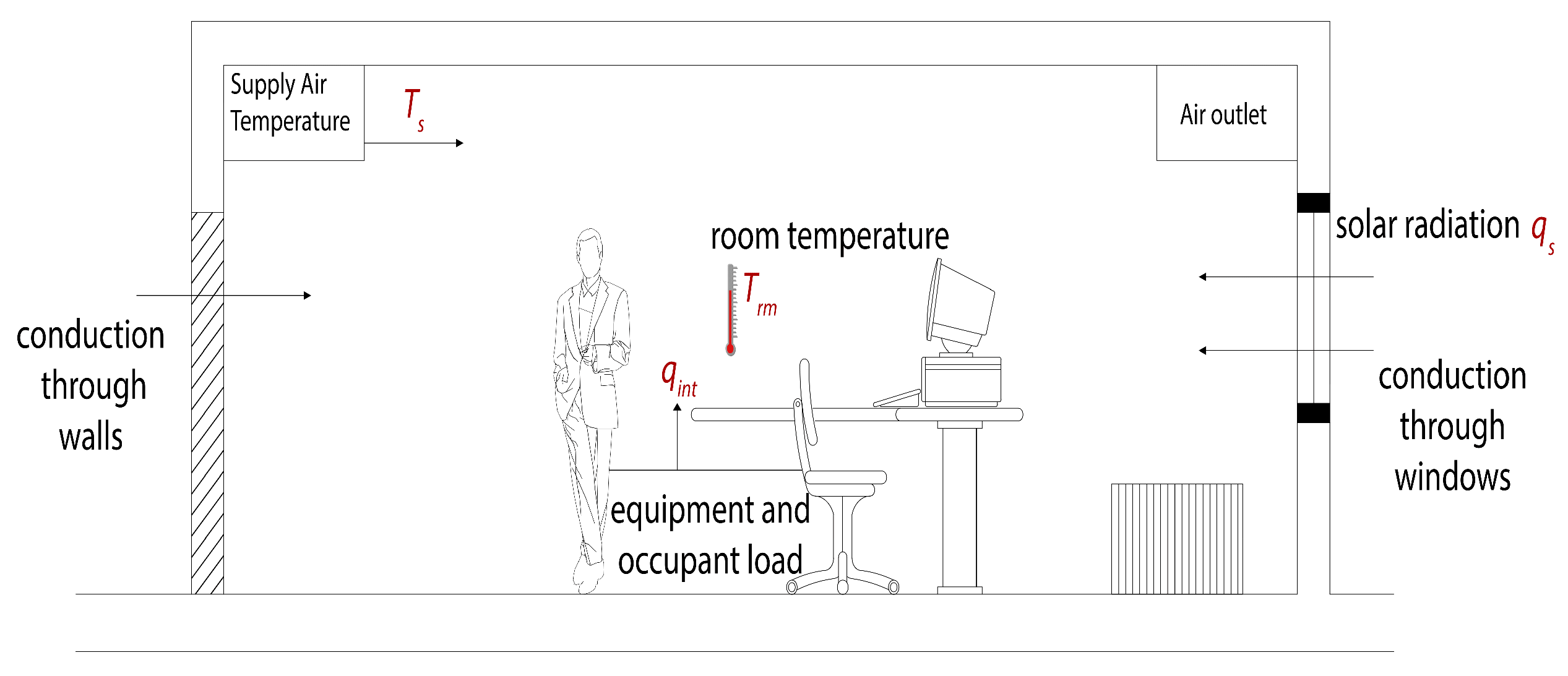
At the room level, we quantify the sources and sinks that affect the temperature change in a room, as shown in Figure 2. The balance in room #i can be defined via

$$\begin{array}{c}{\displaystyle \frac{d{T}_{r{m}_i}}{dt}}=\underset{\mathrm{cooling}\mathrm{load}\mathrm{due}\mathrm{to}\mathrm{HVAC}}{\underbrace{\frac{u_{r{m}_i}}{{\rho }_a{V}_{r{m}_i}}(T_s-T_{r{m}_i})}}+\underset{\mathrm{conduction}\mathrm{through}\mathrm{walls}}{\underbrace{\frac{h_{w{a}_i}{A}_{w{a}_i}}{c_a{\rho }_a{V}_{r{m}_i}}(T_{w{a}_i}-T_{r{m}_i})}}\hfill \\ +\underset{\mathrm{conduction}\mathrm{through}\mathrm{windows}}{\underbrace{\frac{h_{w{d}_i}{A}_{w{d}_i}}{c_a{\rho }_a{V}_{r{m}_i}}(T_{w{d}_i}-T_{r{m}_i})}}+\underset{\mathrm{solar}\mathrm{radiation}}{\underbrace{\frac{q_s}{c_a{\rho }_a{V}_{r{m}_i}}}}+\underset{\mathrm{occupants}\mathrm{and}\mathrm{equipment}}{\underbrace{q_{int}.}}\hfill \end{array}$$

(2)

In Equation (2), $T_{wa}$ and $T_{wd}$ constitute unmeasurable variables. Therefore, the wall and window temperatures are expressed as an affine function of the room and outside air temperature, in line with [30]

$$T_{w{a}_i}=T_{r{m}_i}+\frac{T_{out}-T_{r{m}_i}}{R_{w{a}_i}{A}_{w{a}_i}{h}_{r{m}_i}},$$

(3)

where $R_{wa}=\frac{1}{h_{r{m}_1}{A}_{wa}}+\frac{l}{k_{wa}{A}_{wa}}+\frac{1}{h_{ou{t}_1}{A}_{wa}}$ is the combination of conductive and conductive heat transfer coefficients in [K/W]. Similarly, for the window temperature $T_{wd}$, we have

$$T_{w{d}_i}=T_{r{m}_i}+\frac{T_{out}-T_{r{m}_i}}{R_{w{d}_i}{A}_{w{d}_i}{h}_{w{d}_i}},$$

(4)

where $R_{wd}=\frac{1}{h_{r{m}_2}{A}_{wd}}+\frac{l}{k_{wd}{A}_{wd}}+\frac{1}{h_{ou{t}_2}{A}_{wd}}$ is the thermal resistance in [K/W].

A few standard assumptions have been made to develop Equations (1) and (2): air and water are well-mixed and have the same temperature; there is no heat loss through ducts and pipes in the system; thermal conductivity of walls is constant and the heat transfer through it is one-dimensional.

In Equations (1) and (2), the multiplication of the control input (flow) by the state (temperature) results in a bilinear system. This continuous-time bilinear model is discretized with $\Delta t=10$ min using a backward Euler approach, which is well suited for systems with low sampling rates, such as BMSs [31]. The discretized (bilinear) model is then linearized around the point of 24 °C for the room temperature: since the temperature and input range is quite small, this is sufficient for control purposes [32,33]. The resulting discrete-time linear model can be represented in the state-space structure

$$\begin{array}{cc}\hfill x(k+1)& =Ax\left(k\right)+Bu\left(k\right)+B_{d}d\left(k\right),\hfill \\ \hfill y\left(k\right)& =Cx\left(k\right)+Du\left(k\right),\hfill \end{array}$$

(5)

where $x={\left[\begin{array}{cccc}{T}_{r{m}_1}& T_{r{m}_2}& T_{r{m}_3}& T_{r{m}_4}\end{array}\right]}^T\in {\mathbb{R}}^4$ is the state (comprising the four zone temperatures), $u={\left[\begin{array}{cccc}{u}_{r{m}_1}& u_{r{m}_2}& u_{r{m}_3}& u_{r{m}_4}\end{array}\right]}^T\in {\mathbb{R}}^4$ is the input (comprising the four air flow rates), and $d={\left[\begin{array}{ccc}{T}_{out}& q_s& q_{int}\end{array}\right]}^T\in {\mathbb{R}}^3$ is the disturbance (comprising external temperature, solar radiation and internal gains).

3. Optimization Problem Formulation

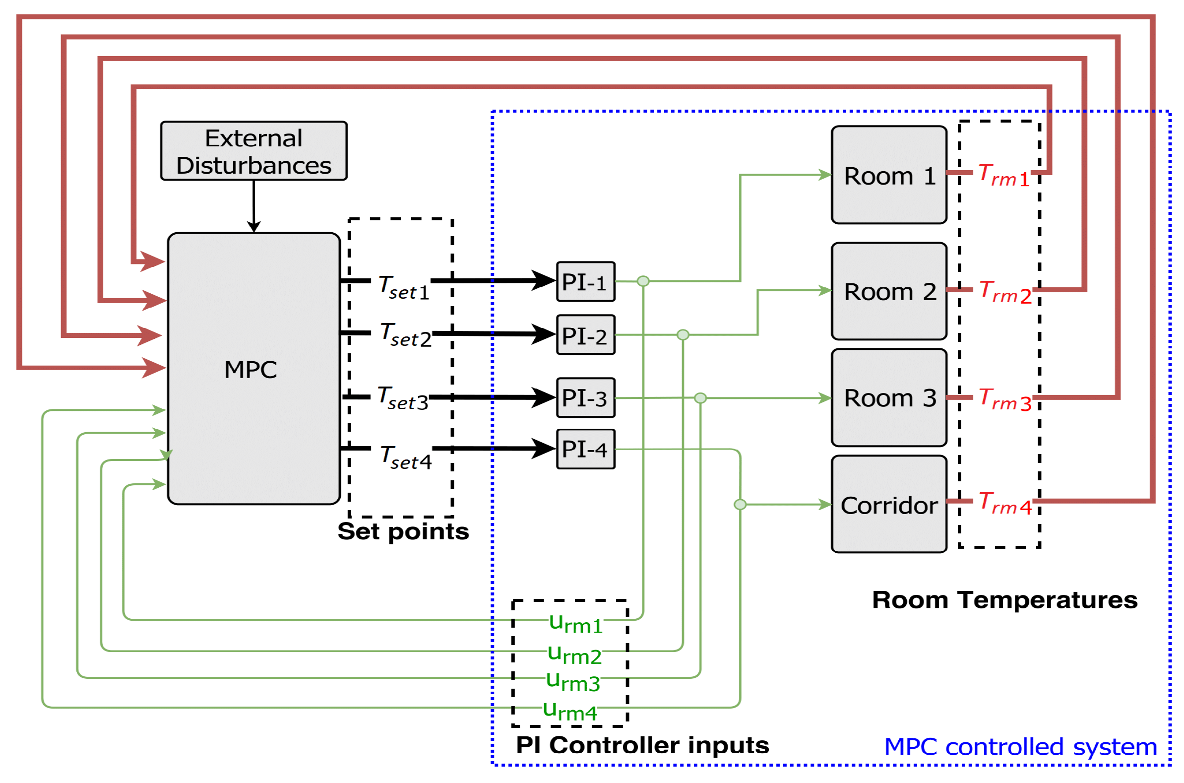
The optimization involves: optimization of the low-level PI controls (in order to achieve acceptable tracking of the set points); optimization of the set-points (in order to minimize energy consumption and thermal discomfort). A schematic of the overall control strategy is represented in Figure 3.

3.1. Optimization for Low-Level Controllers

Four PI controllers, one for each VAV box, are considered: as the purpose of PI control is to achieve tracking with limited energy, we need to quantify the energy consumption of the fan, pump and chiller. With a common duct distributing airflow to all three rooms and the corridor, the total mass airflow $u_a$ blown by the fan is the sum of the individual inlet airflow rates. Therefore, the fan power consumption is [29]

$$\begin{array}{c}\hfill Q_f=u_a\Delta P,\end{array}$$

(6)

where $\Delta P$ is the total pressure increase in the fan in $Pa$. The power by the pump is [29]

$$\begin{array}{c}\hfill Q_p=\frac{u_w{\rho }_{w}gh}{3.6·{10}^6},\end{array}$$

(7)

where $u_w$ is the pump flow capacity, ${\rho }_w$ the density of water, g is gravity acceleration and h is the differential head (the term $3.6·{10}^6$ is for the conversion from J to kWh). Finally, the chiller power $Q_c$ is obtained in (1) by calculating the water temperature drop in the cooling coil. All powers are converted into energies after integration over time.

Eight PI gains (four proportional $K_p$, four integral $K_i$) are be designed through an offline simulation-based optimization via the Matlab (Matlab R2016b, The MathWorks, Inc., Natick, Massachusetts, USA) command ‘fmincon’, to minimize the following cost function:

$$J=\sum _{k=0}^{{\tau }_f}\left(\sum _{i=1}^4{(T_{r{m}_i}\left(k\right)-T_{set}\left(k\right))}^2\right)+{10}^{-2}(Q_f^2+Q_p^2+Q_c^2),$$

where $T_{set}$ is the desired zone temperature and ${\tau }_f$ represents the total duration of the simulation (in this case, 24 h). The cost J formalizes the objective to track the desired set points while minimizing energy consumption: the weight ${10}^{-2}$ was chosen as a trade-off between these goals. The optimized PI gains for each VAV box are given in

Table 1. Auto-tuned PI gains after optimization.

	VAV	VAV	VAV	VAV
Gain	Room 1	Room 2	Room 3	Corridor
$K_p$	7.63	7.63	8.10	6.92
$K_i$	0.66	0.66	0.70	0.65

. It must be noted that, because rooms 1 and 2 have identical size and layout, we have imposed the same PI gains: however, even without such imposition, the result of the optimization was having such gains very close to each other.

3.2. Optimization for Set-Point Control

3.2.1. Thermal Comfort

The sense of thermal comfort of a human is a highly subjective sensation which could be attributed to various factors such as general health, geographical upbringing and general physical composition. Fanger proposed to quantify such factors and created a predictive model for whole body thermal comfort via the PMV index [34]. The PMV index is now standardized in the American Society of Heating, Refrigerating and Air-Conditioning Engineers (ASHRAE) thermal sensation scale [16]: this thermal scale runs from Cold (−3) to Hot (+3) where 0 indicates maximum user comfort.

The equation for Predicted Mean Vote (PMV) index is

$$\mathrm{PMV}=[0.303e^{-0.036M}+0.028]L,$$

(8)

where L is the thermal load, defined as the difference of metabolic heat generation and the calculated heat loss from the body to the actual environmental conditions, assuming optimal comfort conditions:

$$\begin{array}{c}L=M-W-3.96\times {10}^{-8}{f}_{cl}[{(t_{cl}+273)}^4-{(t_r+273)}^4]\hfill \\ -f_{cl}{h}_c(t_{cl}-T_{rm})-3.05[5.73-0.007(M-W)-{\rho }_a]\hfill \\ +0.42[(M-W)-58.15]-0.0173M(5.87-{\rho }_a)\hfill \\ -0.0014M(34-T_{rm}),\hfill \end{array}$$

(9)

where $f_{cl}$ is the clothing factor, $h_c$ is the convective heat transfer coefficient, M is the metabolic rate [W/m${}^2$], ${\rho }_a$ is the vapor pressure of air [kPa], $t_{rm}$ is the room air temperature, $t_{cl}$ is the temperature of the clothing surface [C], $t_r$ is the mean radiant temperature [C], and W is the external work (taken as 0 for office conditions).

The mean radiant temperature is a difficult quantity to measure, since it involves measurement of the wall envelope and window temperature [35]. It is also a highly nonlinear function, which can be computationally expensive when included in the cost of the optimization. To overcome this, Rohles [36] proposed an adapted model of the PMV which expresses the thermal sensation as a function of parameters easily sampled in an office environment, such as air temperature and relative humidity. The boundary conditions of the modified PMV index were: clothing insulation level $I_{cl}=0.6$ clo, metabolic rate M = 70 W/m${}^2$, and air velocity $v_a$ = 0.2 m/s. With these approximations, the PMV equation from (8) can be expressed as a function of Temperature $T_{rm}$ and water vapour pressure ${\rho }_a$, and given by

$${\mathrm{PMV}}_{rm}=a{T}_{rm}+b{\rho }_a-c,$$

(10)

where a, b and c are Rohles’ experimental coefficients, and are dependent on the gender of the occupants. For a male occupant, $a=0.212$, $b=0.293$, $c=5.949$ and for a female it is $a=0.275$, $b=0.255$, $c=8.62$. The simplified PMV index (10) is used in the predictive optimization.

3.2.2. Model Predictive Controller

To account for tracking transients, we augment the system state x with $\overline{x}={\left[\begin{array}{c}{x}^T{x}_c^T\end{array}\right]}^T$, where $x_c\left(k\right)\in {\mathbb{R}}^4$ represents the PI controller states. Substituting for input $u_c\left(k\right)$ in (5), we have

$$\begin{array}{cc}\hfill \overline{x}(k+1)& =A_{in}\overline{x}\left(k\right)+B_{in}e\left(k\right),\hfill \\ \hfill u_c\left(k\right)& =C_{i{n}_u}\overline{x}\left(k\right)+D_{i{n}_u}e\left(k\right),\hfill \\ \hfill y\left(k\right)& =C_{i{n}_y}\overline{x}\left(k\right)+D_{i{n}_y}e\left(k\right),\hfill \end{array}$$

(11)

with $u_c\left(k\right)\in {\mathbb{R}}^4$ being the PI controller inputs and $e\left(k\right)\in {\mathbb{R}}^4$ being the error vector

$$\begin{array}{cc}\hfill A_{in}=\left[\begin{array}{cc}B{C}_c& A\\ A_c& 0\end{array}\right]& B_{in}=\left[\begin{array}{c}B{D}_c\\ B_c\end{array}\right],\hfill \\ \hfill C_{i{n}_u}=\left[\begin{array}{cc}0& C_c\end{array}\right]& D_{i{n}_u}=D_c,\hfill \\ \hfill C_{i{n}_y}=\left[\begin{array}{cc}C& D{C}_c\end{array}\right]& D_{i{n}_y}=D{D}_c.\hfill \end{array}$$

Substituting back for $e\left(k\right)$, we get the overall closed-loop equations with PI controllers

$$\begin{array}{cc}\hfill A_{out}& =A_{in}-B_{in}{(I+D_{i{n}_y})}^{-1}{C}_{i{n}_y},\hfill \\ \hfill B_{out}& =B_{in}-B_{in}{(I+D_{i{n}_y})}^{-1}{D}_{i{n}_y},\hfill \\ \hfill C_{ou{t}_u}& =C_{i{n}_u}-D_{i{n}_y}{(I+D_{i{n}_y})}^{-1}{C}_{i{n}_u},\hfill \end{array}$$

$$\begin{array}{cc}\hfill D_{ou{t}_u}& =D_{i{n}_u}-D_{i{n}_u}{(I+D_{i{n}_y})}^{-1}{D}_{i{n}_u},\hfill \\ \hfill C_{ou{t}_y}& ={(I+D_{i{n}_y})}^{-1}{C}_{i{n}_y},\hfill \\ \hfill D_{ou{t}_y}& ={(I+D_{i{n}_y})}^{-1}{D}_{i{n}_y},\hfill \end{array}$$

(12)

which finally gives us the complete state space dynamics of the closed-loop system (the blue dashed box in Figure 3)

$$\begin{array}{cc}\hfill \overline{x}(k+1)& =A_{out}\overline{x}\left(k\right)+B_{out}w\left(k\right)+B_{d}d\left(k\right),\hfill \\ \hfill u_c\left(k\right)& =C_{ou{t}_u}\overline{x}\left(k\right)+D_{ou{t}_u}w\left(k\right),\hfill \\ \hfill y\left(k\right)& =C_{ou{t}_y}\overline{x}\left(k\right)+D_{ou{t}_y}w\left(k\right),\hfill \end{array}$$

(13)

where $w\left(k\right)$ is a vector of set-point temperatures with $w={\left[T_{se{t}_1}{T}_{se{t}_2}{T}_{se{t}_3}{T}_{se{t}_4}\right]}^T$.

Using (10) and the closed loop state space derived in (11), we formulate the optimization for the MPC as follows:

$$\begin{array}{cc}\hfill \underset{\tilde{w}\left(k\right)}{\mathrm{minimize}}\sum _{k=0}^{N_p-1}& (\underset{\mathrm{energy}\mathrm{minimization}}{\underbrace{\left|\right|K_u\Delta u{\left|\right|}_1}}+\hfill \\ & \underset{\mathrm{comfort}\mathrm{maximization}}{\underbrace{\left|\right|K_{pmv}(PM{V}_{rm}\left(k\right)-s\left(k\right)){\left|\right|}_1}}),\hfill \\ \hfill \mathrm{subject}\mathrm{to}:& \left(11\right)\hfill \\ \hfill -0.2\le & s\le 0.2,0.01\le u\le 2,\hfill \\ \hfill 18\le & y\le 26,-0.5\le \Delta u\le 0.5,\hfill \end{array}$$

where $\tilde{w}$ indicates the sequence of set points w along the prediction horizon, and s is a vector of slack variables for the PMV. We set a prediction horizon of $N_p=10$ for the optimization problem.

4. Validation

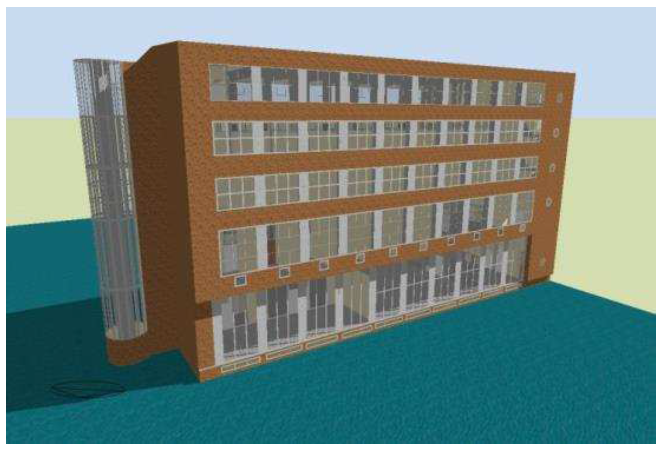
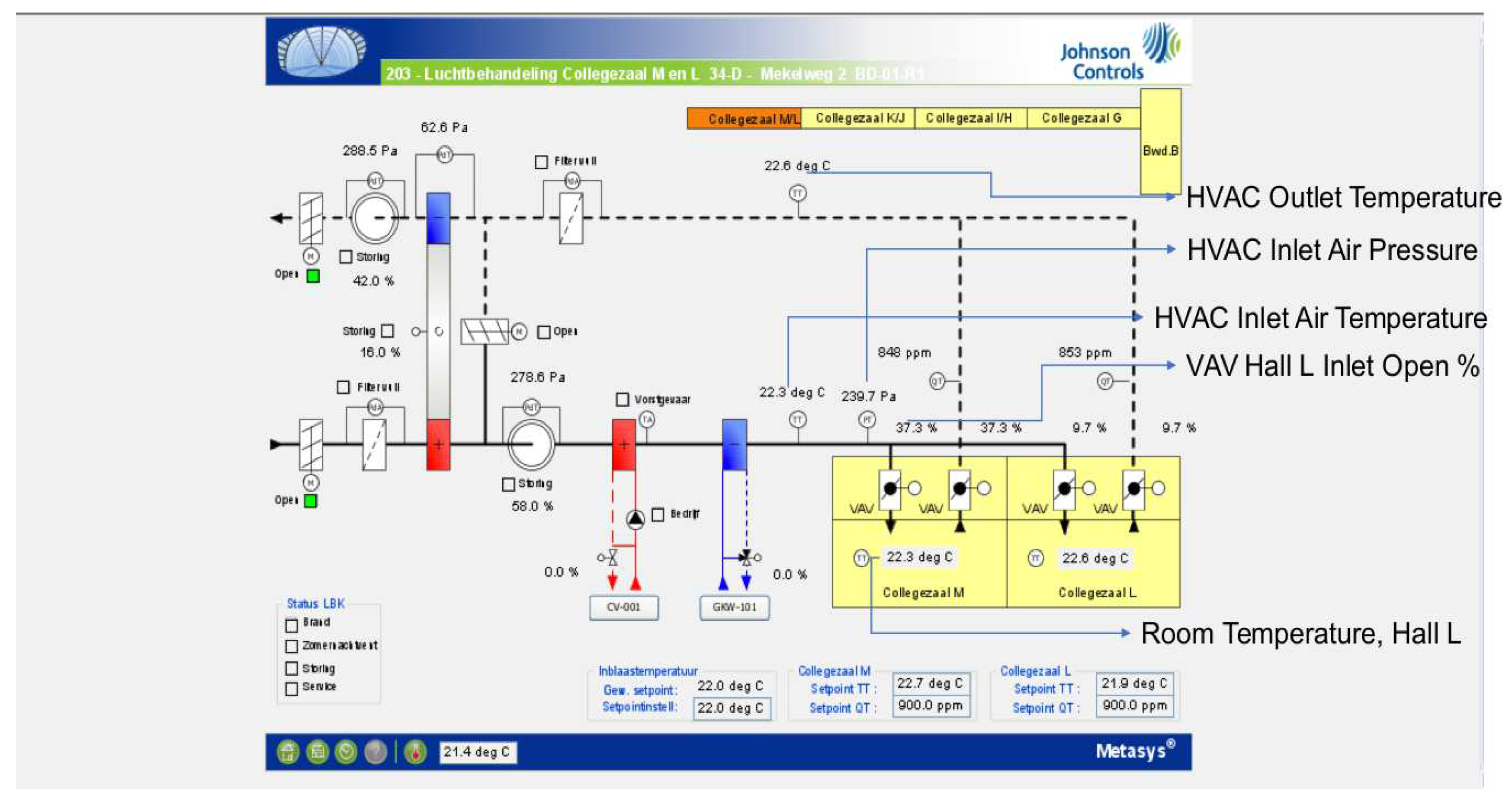
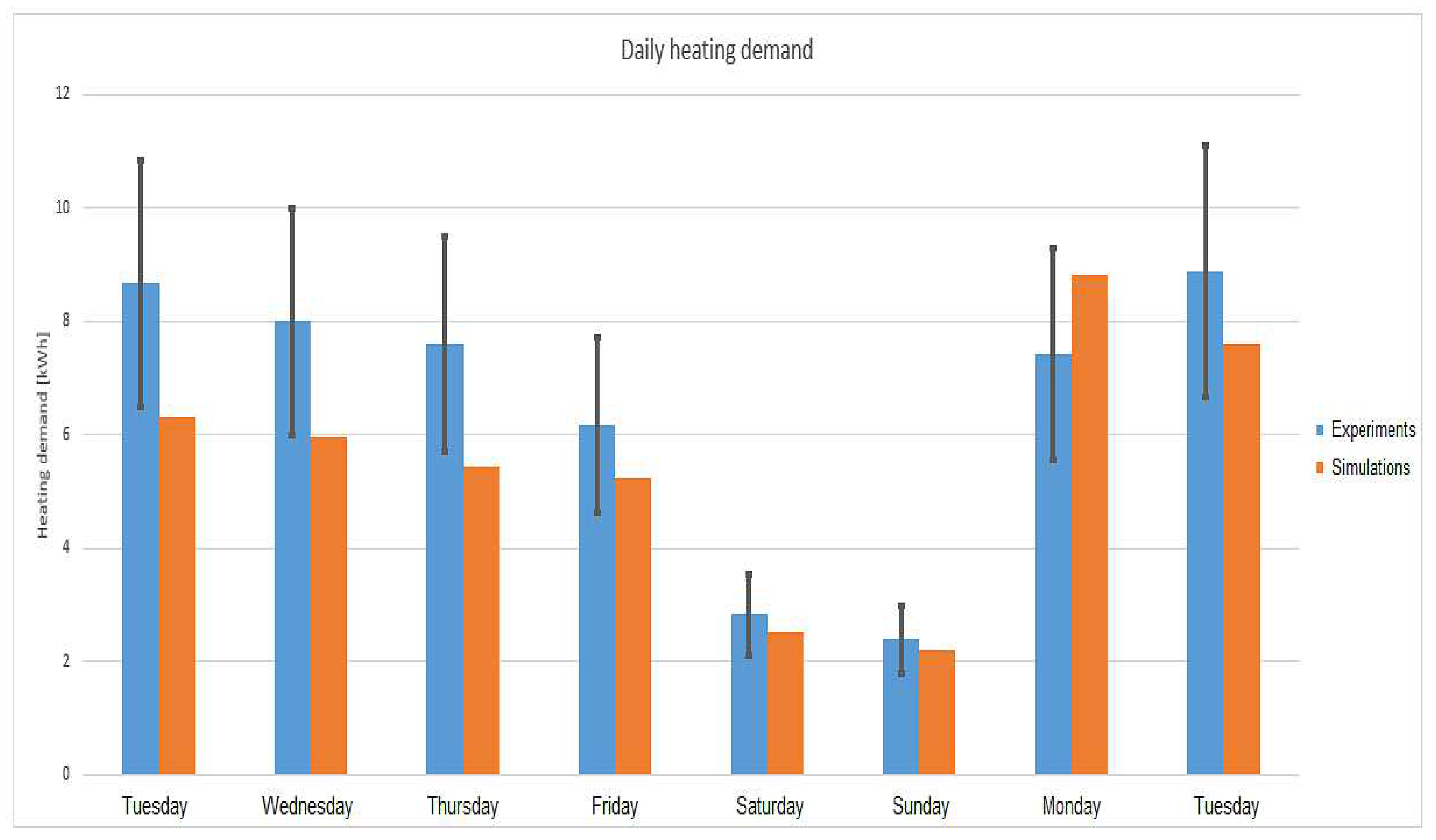
To test the real-world feasibility of this approach, we model the building facility at TU Delft using EnergyPlus (EnergyPlus 7.0.0, Department of Energy’s (DOE) Building Technologies Office (BTO), Washington, DC, USA) [26], as shown in Figure 4. EnergyPlus is a simulation program that allows simulation the energy consumption for HVAC loads as well as water usage within buildings. Upon constructing an EnergyPlus model of the building, this model was compared with the actual energy usage collected by the Building Management System of the faculty, which is MetaSys (Metasys 9.0, Johnson Controls Inc., Cork, Ireland) by Johnson Controls (a sample interface is shown in Figure 5). Figure 6 shows the experimental simulation of the EnergyPlus model to compare the daily heating demand of the actual and EnergyPlus building.

For the validation, the following simplifications were made. The chiller power was approximated by the electricity consumption of the entire building by scaling it proportionally to the ratio between the volume of the building and the volume of the test rooms and corridor; the damper proportion was kept constant according to information received from the facility management (70:30% mixing of fresh and return air). Finally, together with the EnergyPlus model, a Matlab model of the building was constructed from (1) and (2) taking into account interactions among rooms (the equations for the entire model cannot be shown due to limited space): all the parameters in the Matlab model have been derived based on physical properties (density, thermal capacitance, convective heat coefficients). The temperature for the chiller and the cooling coil have been selected as suggested by the facility management. The parameters were further tuned using a system identification procedure, as proposed by [30].

5. Simulations

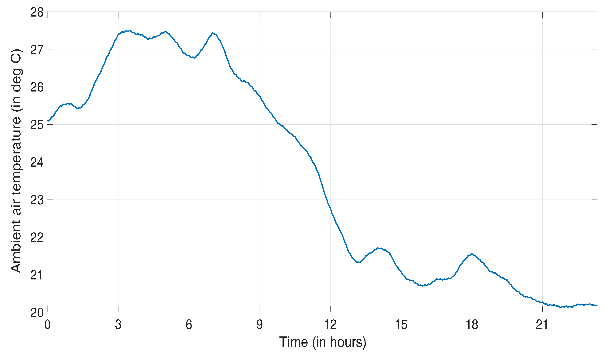
The proposed MPC + Autotuned PI strategy is simulated in Matlab and interfaced with EnergyPlus. To highlight energy savings, this strategy is compared with a baseline control that tracks a constant set point of 24 °C. Simulations are run for a span of 24 h, with weather profile taken from 19 June 2017, as shown in Figure 7. Please note that the strategy we used has been taken from the actual strategy used in the University building (constant set point and constant 70:30% mixing of fresh and return air). We agree that smarter strategies are in general possible and would lead to different numerical results.

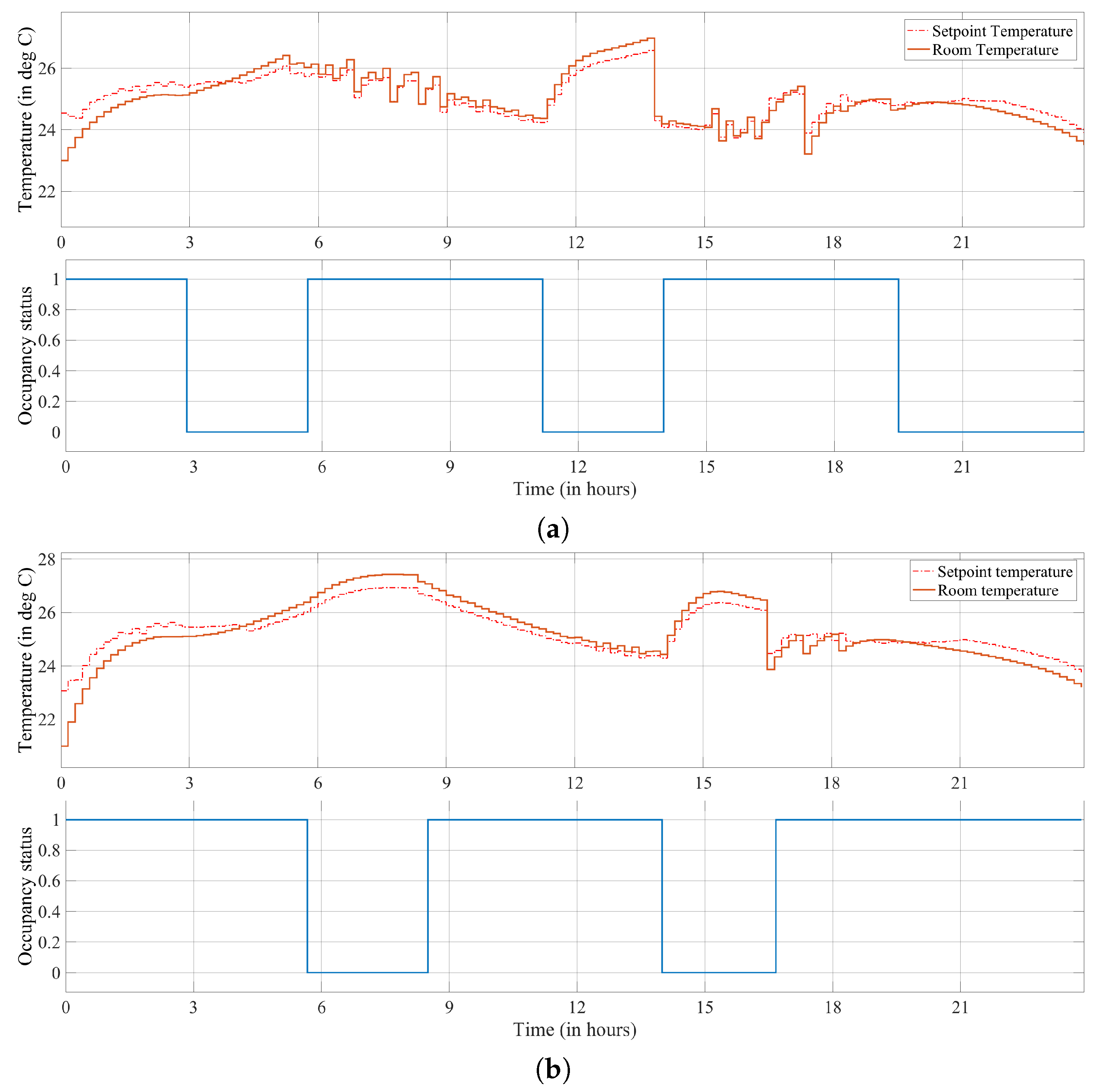
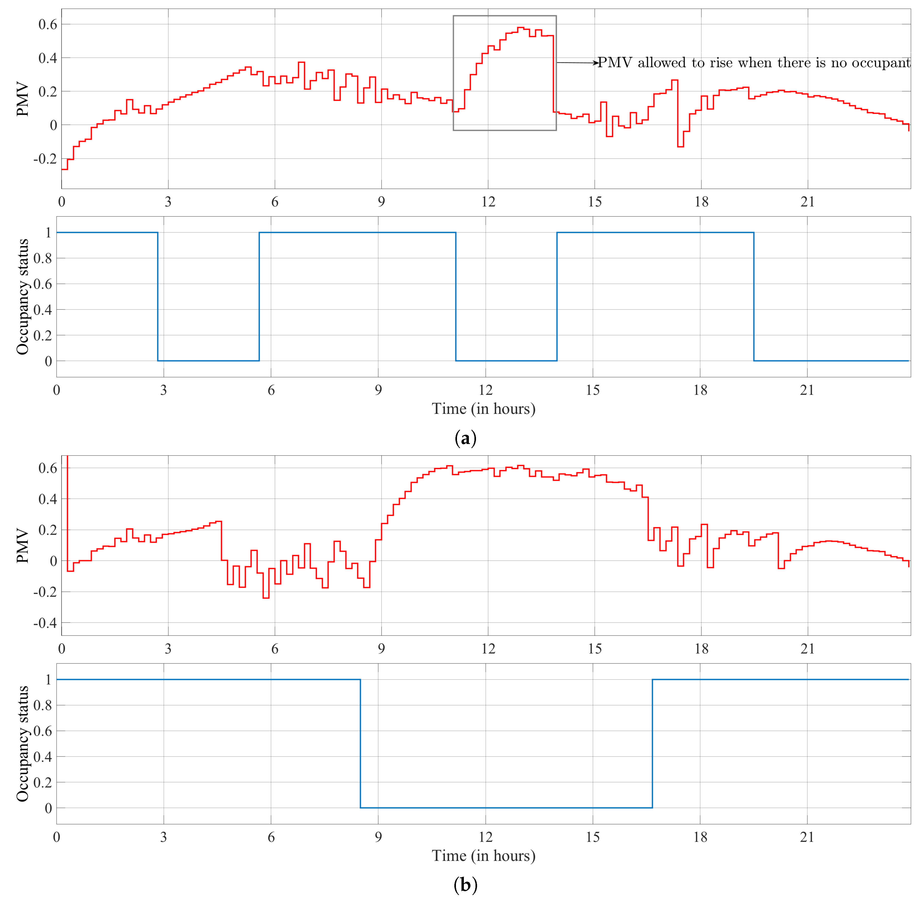
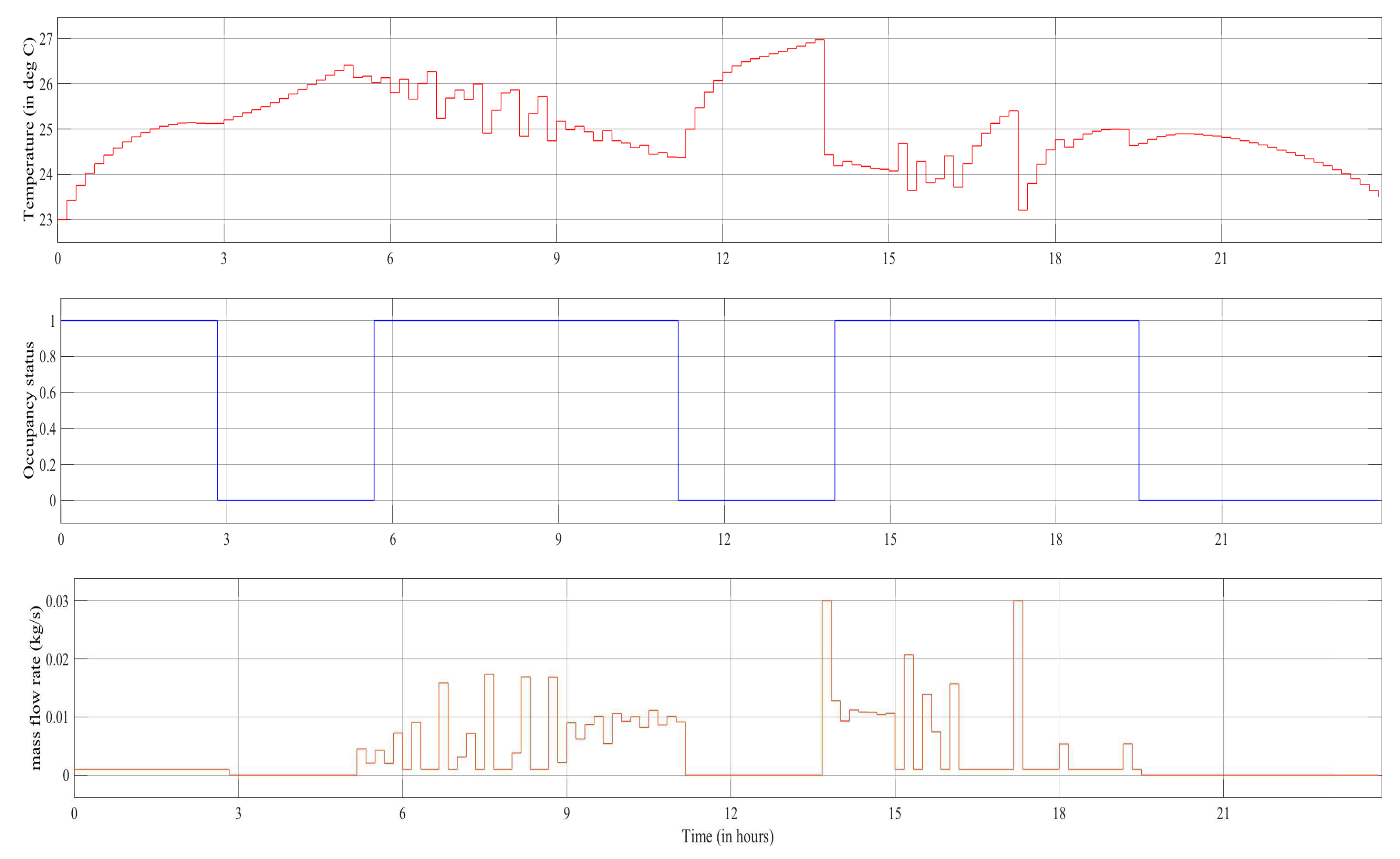
Figure 8 and Figure 9 show the temperature tracking and PMV profile for two rooms (the other room and the corridor have a similar behavior to the one shown here). The error in set-point tracking is less than ±0.5 °C, which is acceptable due to quantized measurements provided by the sensors simulated in EnergyPlus. When occupants are present in a room, it can be seen that PMV is mostly maintained within $\pm 0.2$, which is within the prescribed ASHRAE limits of 0.5. It can also be noted from Figure 10 that the effort is to maintain comfort while having minimal supply air whenever possible.

The most interesting behavior, which justifies the occupancy-based effort of this work occurs when occupants are not present in a room: in this case, the PMV is allowed to increase (note that the supply air is zero, as shown in Figure 10). Basically, when no people are inside a room, the temperature evolution in the room/corridor is mainly due to conduction through the walls and windows.

In this work, it has been assumed that the occupancy schedule can be forecast. In principle, such forecasting is possible based on the schedule of the lectures: in fact, at TU Delft, the lecture rooms are open during lecture times and closed otherwise. We acknowledge that, in more general settings, such forecasting may be not trivial, c.f. the excellent survey [37]. It can be noted that, because the optimization is based on minimization of PMV, a pre-cooling action is automatically implemented to allow people to find a good climate when they are back. In fact, Figure 10) reveals that around half an hour before people arrive the air flow is turned on again (the other rooms exhibit a similar behavior).

Table 2. Air pushed in the rooms in [kg] and total energy consumption in [kW] for a simulation of one day.

Controller	Total Airflow (kg)	Consumption (kW)
Baseline PI	1877.1	12.77
MPC + optimized PI	1132.5 (−39.7%)	7.70 (−39.7%)

shows the comparison of power consumption for the variable supply fan for the baseline PI strategy with the PI with MPC. We notice that, while the optimization only accounted for reduction in fan power, the pump at the chiller side also had a reduced load due to lowered cooling demand. Therefore, there was a significant reduction in the power consumed by the pump as well. Overall, almost $40\%$ reduction in energy consumption of the fan is achieved. Please note that the energy consumption of the fan can be derived from the mass flow rate trend, and it is therefore not reported to avoid including extra figures. In addition, we noticed that the pump and chiller also had a reduced energy consumption due to lowered cooling demand.

6. Conclusions and Future Work

This paper presented an integrated framework to model the set-point and low-level control of a multi-component HVAC system. Starting from a physics-based modelling, a system-of-subsystems dynamic model was used to design a set of strategies that integrate set-point predictive control and low-level PI control. One of the advantages of the proposed control strategy is that, by embedding the PI dynamics in the predictive structure, we are able to account for tracking transients, which are particularly useful if the HVAC is switched on and off depending on occupancy patterns. In addition, we do not disrupt the standard hierarchy of controllers typical of building automation systems. The lower level controllers are auto-tuned so as to track the set points with limited energy consumption; the set points generated by the higher level controller were generated in such a way that comfort was maximized and overall system energy minimized. Energy savings of around 40% have been reported, by using a three-room test case at the Delft University of Technology validated in EnergyPlus using real-life data. Future work will include extension of this design principle so as to consider a stochastic MPC with chance constraints to increase flexibility of the strategy to varying weather and heat load conditions.

References

- Pérez-Lombard, L.; Ortiz, J.; Pout, C. A review on buildings energy consumption information. Energy Build. 2008, 40, 394–398. [Google Scholar] [CrossRef]
- Knight, I. Assessing Electrical Energy Use in HVAC Systems. 2012. Available online: http://www.rehva.eu/fileadmin/hvac-dictio/01-2012/assessing-electrical-energy-use-in-hvac-systems_rj1201.pdf (accessed on 15 August 2018).
- Wemhoff, A. Calibration of HVAC equipment PID coefficients for energy conservation. Energy Build. 2012, 45, 60–66. [Google Scholar] [CrossRef]
- Schicktanz, M.; Nunez, T. Modelling of an adsorption chiller for dynamic system simulation. Int. J. Refrig. 2009, 32, 588–595. [Google Scholar] [CrossRef]
- Teitel, M.; Levi, A.; Zhao, Y.; Barak, M.; Bar-lev, E.; Shmuel, D. Energy saving in agricultural buildings through fan motor control by variable frequency drives. Energy Build. 2008, 40, 953–960. [Google Scholar] [CrossRef]
- Koh, J.; Zhai, J.Z.; Rivas, J.A. Comparative energy analysis of VRF and VAV systems under cooling mode. In Proceedings of the ASME 3rd International Conference on Energy Sustainability, ES2009, San Francisco, CA, USA, 19–23 July 2009; Volume 1, pp. 411–418. [Google Scholar]
- Henze, G.P.; Florita, A.R.; Brandemuehl, M.J.; Felsmann, C.; Cheng, H. Advances in near-optimal control of passive building thermal storage. J. Sol. Energy Eng. 2010, 132, 021009. [Google Scholar] [CrossRef]
- Wang, S.; Ma, Z. Supervisory and optimal control of building HVAC systems: A review. HVAC R Res. 2008, 14, 3–32. [Google Scholar] [CrossRef]
- Ma, Z.; Wang, S.; Xu, X.; Xiao, F. A supervisory control strategy for building cooling water systems for practical and real time applications. Energy Convers. Manag. 2008, 49, 2324–2336. [Google Scholar] [CrossRef]
- Nassif, N.; Moujaes, S. A cost-effective operating strategy to reduce energy consumption in a hvac system. Int. J. Energy Res. 2008, 32, 543–558. [Google Scholar] [CrossRef]
- Afram, A.; Janabi-Sharifi, F. Theory and applications of HVAC control systems—A review of model predictive control (MPC). Build. Environ. 2014, 72, 343–355. [Google Scholar] [CrossRef]
- Kontes, G.D.; Giannakis, G.I.; Kosmatopoulos, E.B.; Rovas, D.V. Adaptive-fine tuning of building energy management systems using co-simulation. In Proceedings of the 2012 IEEE International Conference on Control Applications, Dubrovnik, Croatia, 3–5 October 2012; pp. 1664–1669. [Google Scholar]
- Endel, P.; Holub, O.; Berka, J. Adaptive quantile estimation in performance monitoring of building automation systems. In Proceedings of the 2016 European Control Conference (ECC), Aalborg, Denmark, 29 June–1 July 2016; pp. 1189–1194. [Google Scholar]
- Giannakis, G.I.; Kontes, G.D.; Kosmatopoulos, E.B.; Rovas, D.V. A model-assisted adaptive controller fine-tuning methodology for efficient energy use in buildings. In Proceedings of the 2011 19th Mediterranean Conference on Control Automation (MED), Corfu, Greece, 20–23 June 2011; pp. 49–54. [Google Scholar]
- Brager, G.S.; De Dear, R. Climate, Comfort, & Natural Ventilation: A New Adaptive Comfort Standard for ASHRAE Standard 55; American Society of Heating, Refrigerating and air-Conditioning Engineers: Atlanta, GA, USA, 2001. [Google Scholar]
- ASHRAE. ANSI/ASHRAE Standard 55-2010: Thermal Environmental Conditions for Human Occupancy; American Society of Heating, Refrigerating and air-Conditioning Engineers: Atlanta, GA, USA, 2010. [Google Scholar]
- Mirakhorli, A.; Dong, B. Occupancy behavior based model predictive control for building indoor climate—A critical review. Energy Build. 2016, 129, 499–513. [Google Scholar] [CrossRef]
- Baldi, S.; Korkas, C.D.; Lv, M.; Kosmatopoulos, E.B. Automating occupant-building interaction via smart zoning of thermostatic loads: A switched self-tuning approach. Appl. Energy 2018, 231, 1246–1258. [Google Scholar] [CrossRef]
- Oldewurtel, F.; Parisio, A.; Jones, C.N.; Gyalistras, D.; Gwerder, M.; Stauch, V.; Lehmann, B.; Morari, M. Use of model predictive control and weather forecasts for energy efficient building climate control. Energy Build. 2012, 45, 15–27. [Google Scholar] [CrossRef] [Green Version]
- Dong, B.; Lam, K.P. A real-time model predictive control for building heating and cooling systems based on the occupancy behavior pattern detection and local weather forecasting. In Building Simulation; Springer: Berlin, Germany, 2014; Volume 7, pp. 89–106. [Google Scholar]
- Pcolka, M.; Zacekova, E.; Robinett, R.; Celikovsky, S.; Sebek, M. Economical nonlinear model predictive control for building climate control. In Proceedings of the American Control Conference (ACC), Portland, OR, USA, 4–6 June 2014; pp. 418–423. [Google Scholar]
- Klaučo, M. Modeling of the Closed-Loop System with a Set of PID Controllers; Slovak University of Technology: Bratislava, Slovakia, 2016. [Google Scholar]
- Oldewurtel, F.; Sturzenegger, D.; Morari, M. Importance of occupancy information for building climate control. Appl. Energy 2013, 101, 521–532. [Google Scholar] [CrossRef]
- Sturzenegger, D.; Gyalistras, D.; Morari, M.; Smith, R.S. Model Predictive Climate Control of a Swiss Office Building: Implementation, Results, and Cost–Benefit Analysis. IEEE Trans. Control Syst. Technol. 2016, 24, 1–12. [Google Scholar] [CrossRef]
- Killian, M.; Kozek, M. Implementation of cooperative Fuzzy model predictive control for an energy-efficient office building. Energy Build. 2018, 158, 1404–1416. [Google Scholar] [CrossRef]
- EnergyPlus Official Website. Available online: https://energyplus.net (accessed on 21 June 2017).
- Baldi, S.; Michailidis, I.; Ravanis, C.; Kosmatopoulos, E.B. Model-based and model-free “plug-and-play” building energy efficient control. Appl. Energy 2015, 154, 829–841. [Google Scholar] [CrossRef]
- Baldi, S.; Karagevrekis, A.; Michailidis, I.T.; Kosmatopoulos, E.B. Joint energy demand and thermal comfort optimization in photovoltaic-equipped interconnected microgrids. Energy Convers. Manag. 2015, 101, 352–363. [Google Scholar] [CrossRef] [Green Version]
- Satyavada, H.; Baldi, S. An integrated control-oriented modelling for HVAC performance benchmarking. J. Build. Eng. 2016, 6, 262–273. [Google Scholar] [CrossRef] [Green Version]
- Wu, S.; Sun, J.Q. A physics-based linear parametric model of room temperature in office buildings. Build. Environ. 2012, 50, 1–9. [Google Scholar] [CrossRef]
- Baldi, S.; Yuan, S.; Endel, P.; Holub, O. Dual estimation: Constructing building energy models from data sampled at low rate. Appl. Energy 2016, 169, 81–92. [Google Scholar] [CrossRef]
- Maasoumy, M.; Sangiovanni-Vincentelli, A. Total and peak energy consumption minimization of building HVAC systems using model predictive control. IEEE Des. Test Comput. 2012, 29, 26–35. [Google Scholar] [CrossRef]
- Lauro, F.; Longobardi, L.; Panzieri, S. An adaptive distributed predictive control strategy for temperature regulation in a multizone office building. In Proceedings of the 2014 IEEE International Workshop on Intelligent Energy Systems (IWIES), San Diego, CA, USA, 5–8 October 2014; pp. 32–37. [Google Scholar]
- Fanger, P.O. Calculation of thermal comfort, Introduction of a basic comfort equation. ASHRAE Trans. 1967, 73, III–4. [Google Scholar]
- Michailidis, I.T.; Baldi, S.; Pichler, M.F.; Kosmatopoulos, E.B.; Santiago, J.R. Proactive control for solar energy exploitation: A german high-inertia building case study. Appl. Energy 2015, 155, 409–420. [Google Scholar] [CrossRef] [Green Version]
- Rohles, J.; Frederick, H. Thermal sensations of sedentary man in moderate temperatures. Hum. Fact. 1971, 13, 553–560. [Google Scholar] [CrossRef] [PubMed]
- Nguyen, T.A.; Aiello, M. Energy intelligent buildings based on user activity: A survey. Energy Build. 2013, 56, 244–257. [Google Scholar] [CrossRef] [Green Version]
Figure 1.
Scheme of the test case Heating, Ventilation and Air-Conditioning system.
Figure 2.
Scheme of the Heating, Ventilation and Air-Conditioning room test case.
Figure 3.
Scheme of proposed control strategy. Note that the feedback of the Proportional-Integral (PI) controllers creates a nested loop with the Model Predictive Control (MPC) layer.
Figure 4.
Model of Tower C at TU Delft developed using DesignBuilder and simulated in EnergyPlus.
Figure 5.
Screenshot of the Building Management System interface of Tower C.
Figure 6.
Validation of daily heating demand in EnergyPlus.
Figure 7.
Ambient weather temperature for 19 June 2017.
Figure 8.
(a) temperature profile and set-point tracking, Room 1; (b) temperature profile and set-point tracking, Room 2.
Figure 9.
(a) evolution of PMV vs. Occupancy, Room 1; (b) evolution of PMV vs. Occupancy, Room 3.
Figure 10.
Input air flow, Room 1 (notice the pre-cooling action).