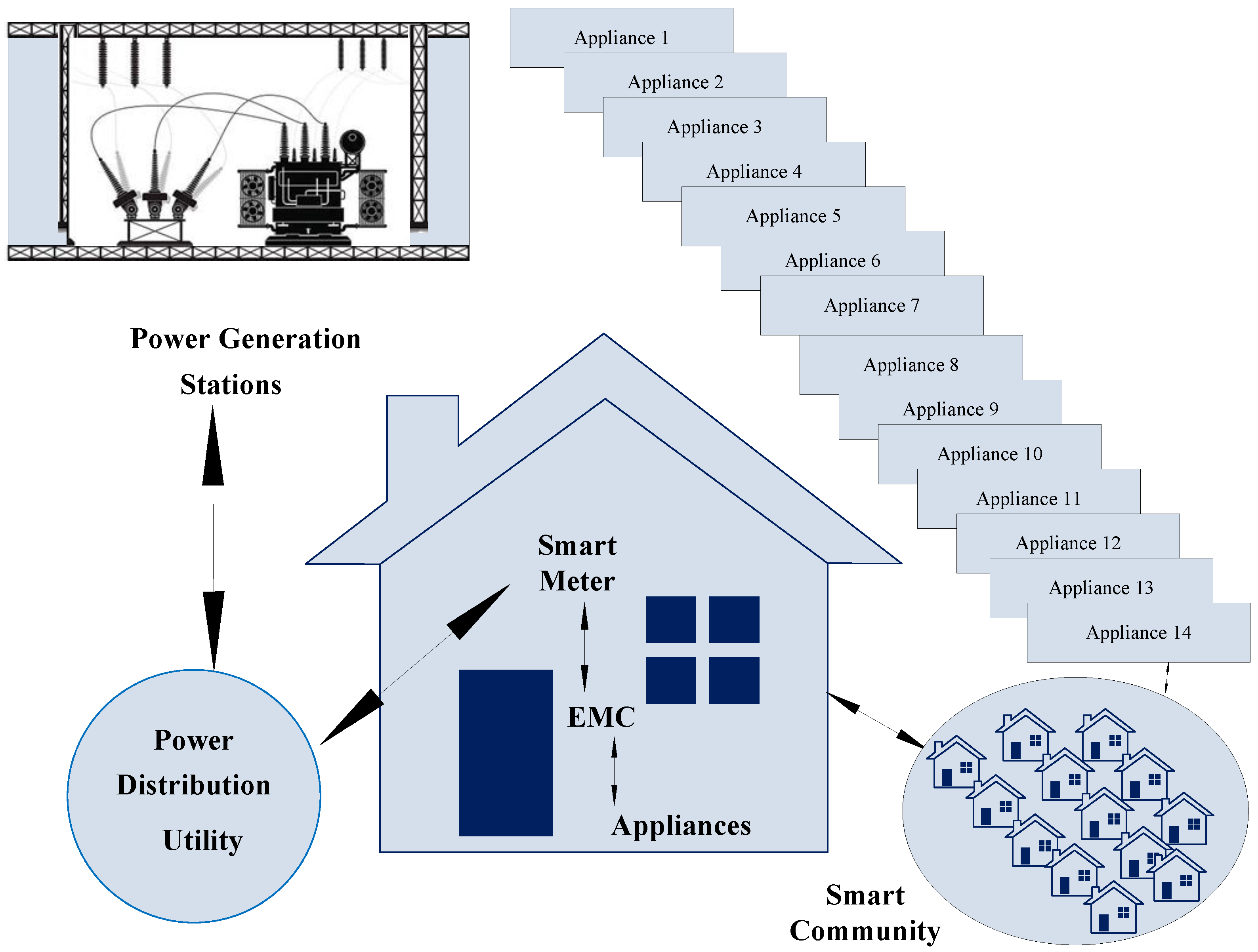
Figure 1.
Proposed system model.
Figure 1.
Proposed system model.
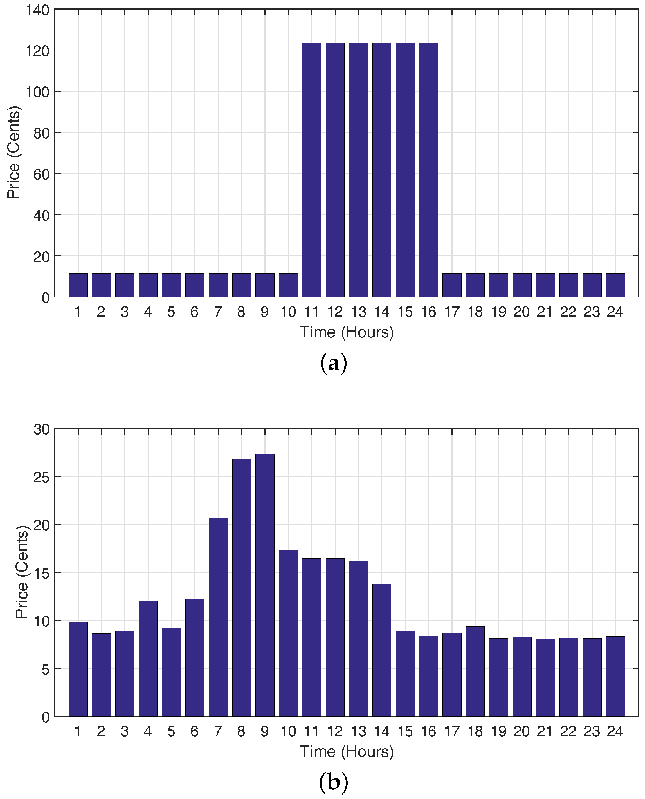
Figure 2.
Pricing tariff. (a) Critical peak pricing.; (b) Real time pricing.
Figure 2.
Pricing tariff. (a) Critical peak pricing.; (b) Real time pricing.
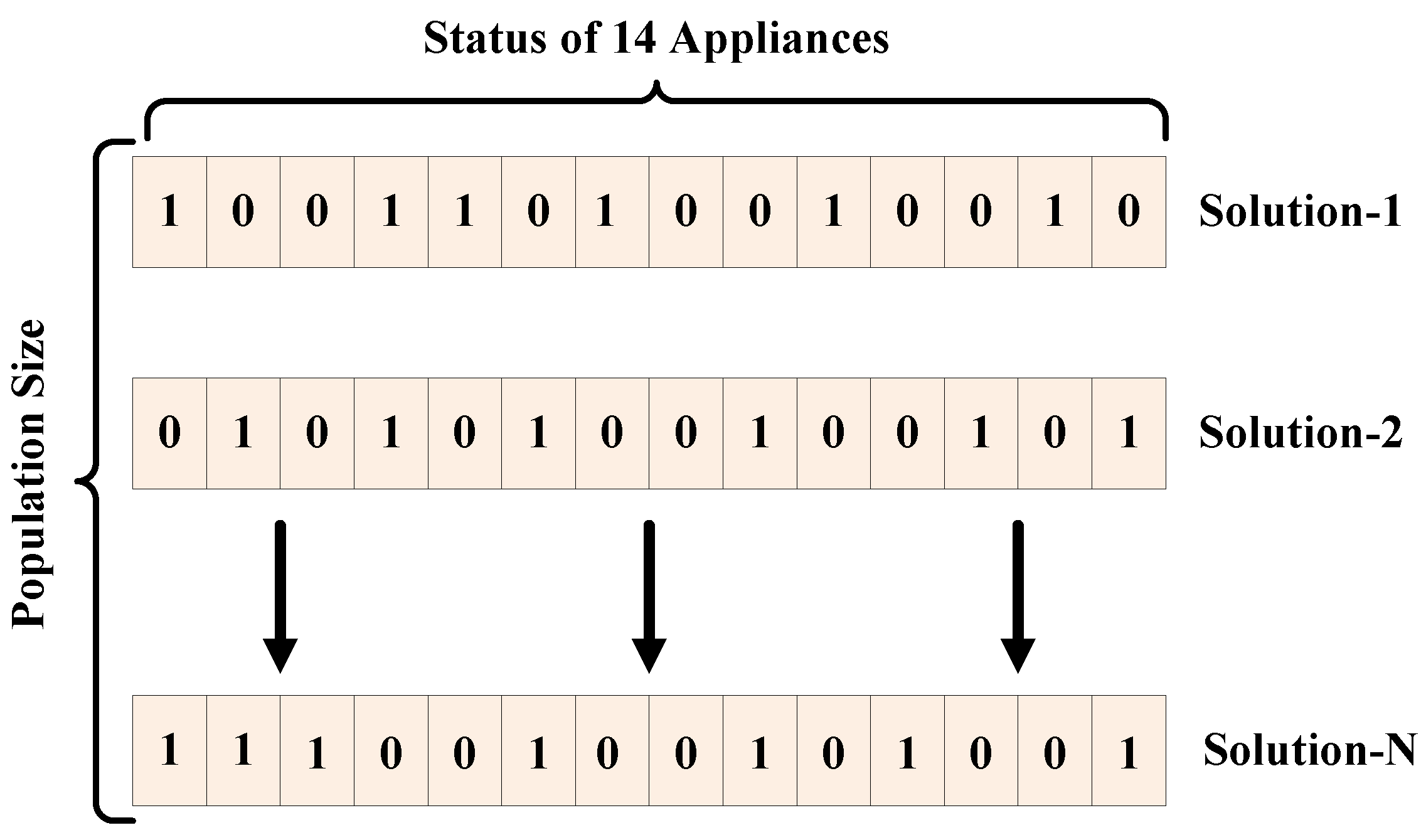
Figure 3.
Hybrid bacterial flower pollination algorithm numerical example.
Figure 3.
Hybrid bacterial flower pollination algorithm numerical example.
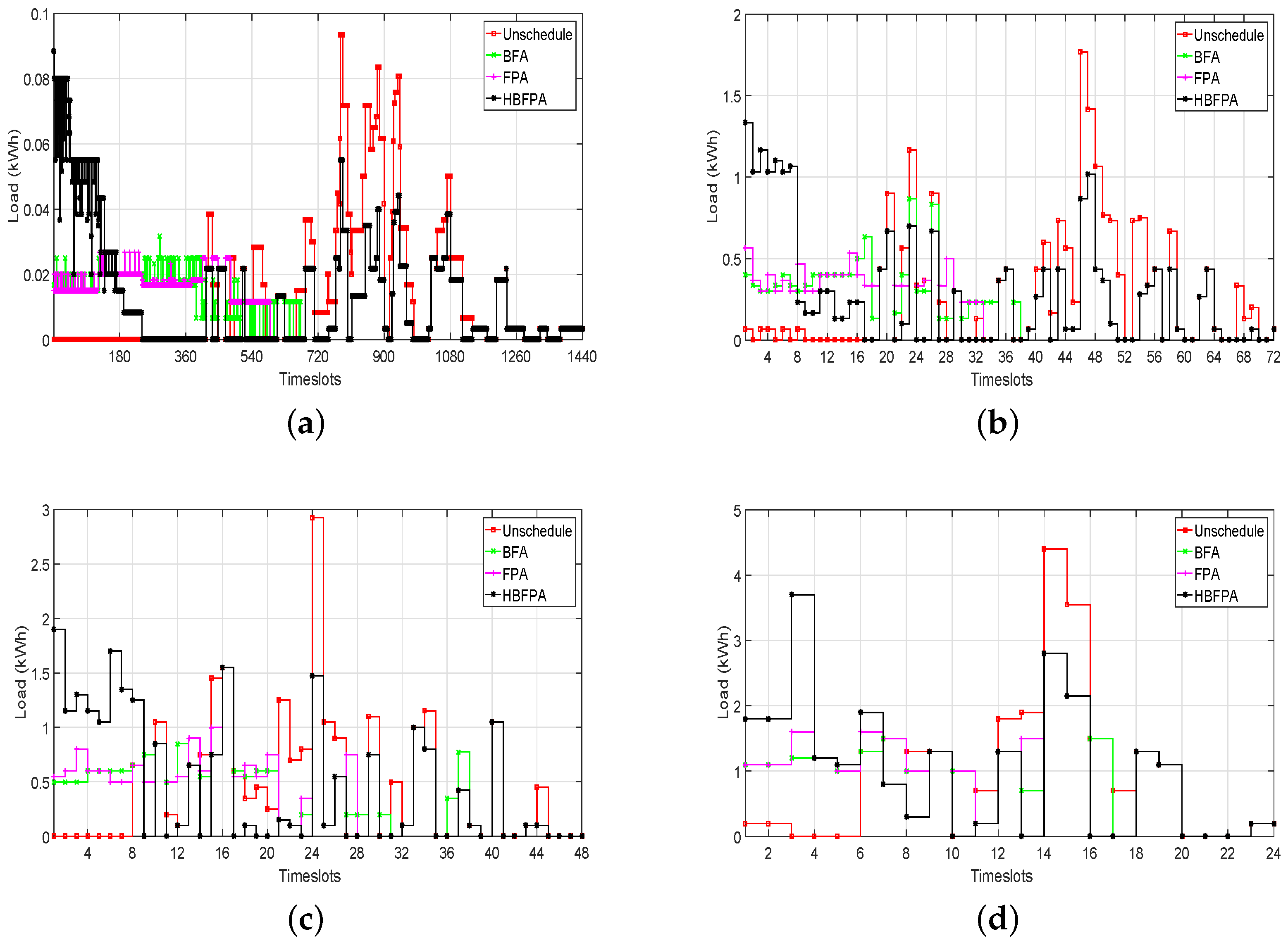
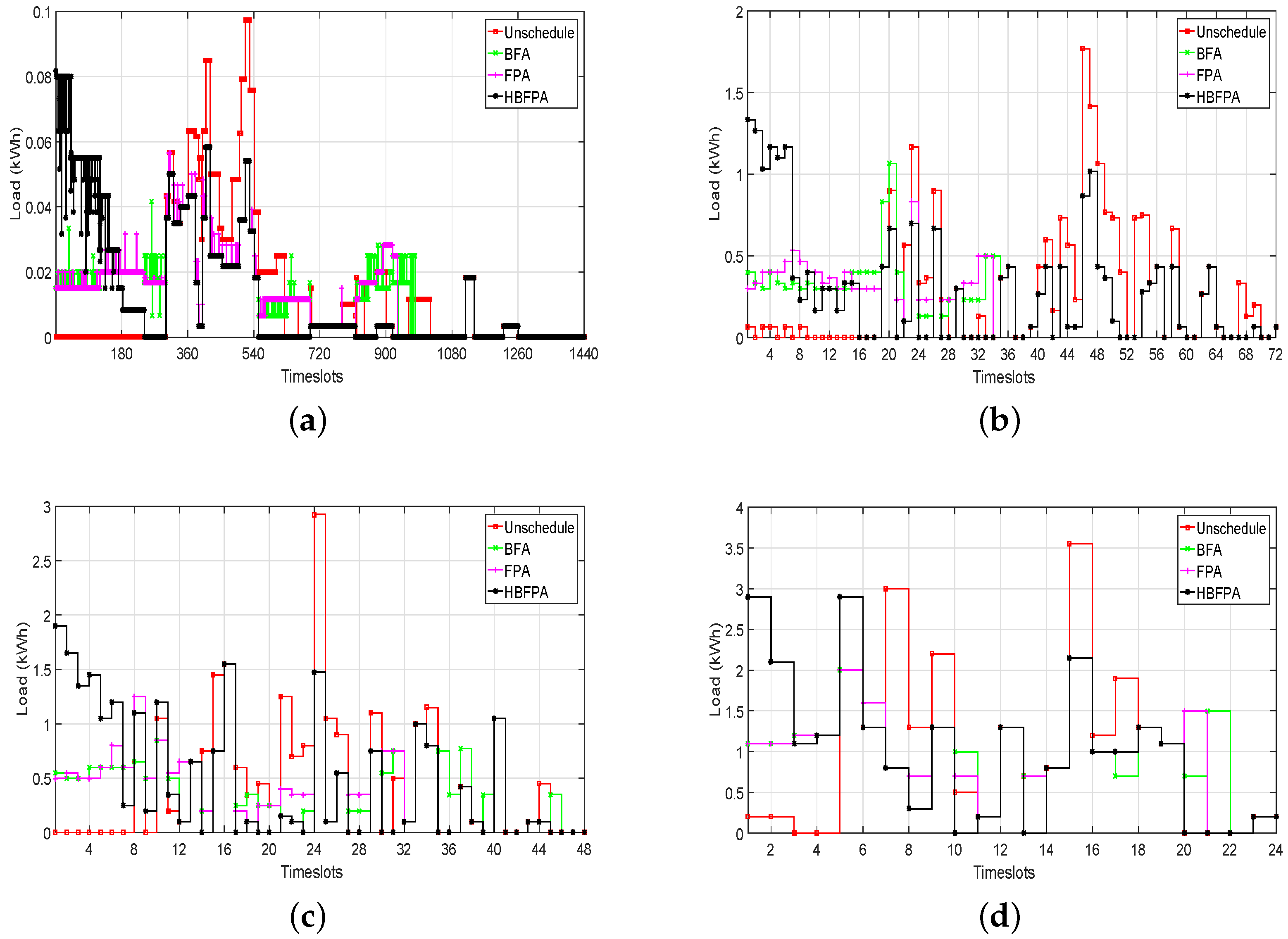
Figure 4.
Load for single home using critical peak pricing. (a) load using operational time interval of 1 min; (b) load using operational time interval of 20 min; (c) load using operational time interval of 30 min; (d) load using operational time interval of 60 min.
Figure 4.
Load for single home using critical peak pricing. (a) load using operational time interval of 1 min; (b) load using operational time interval of 20 min; (c) load using operational time interval of 30 min; (d) load using operational time interval of 60 min.
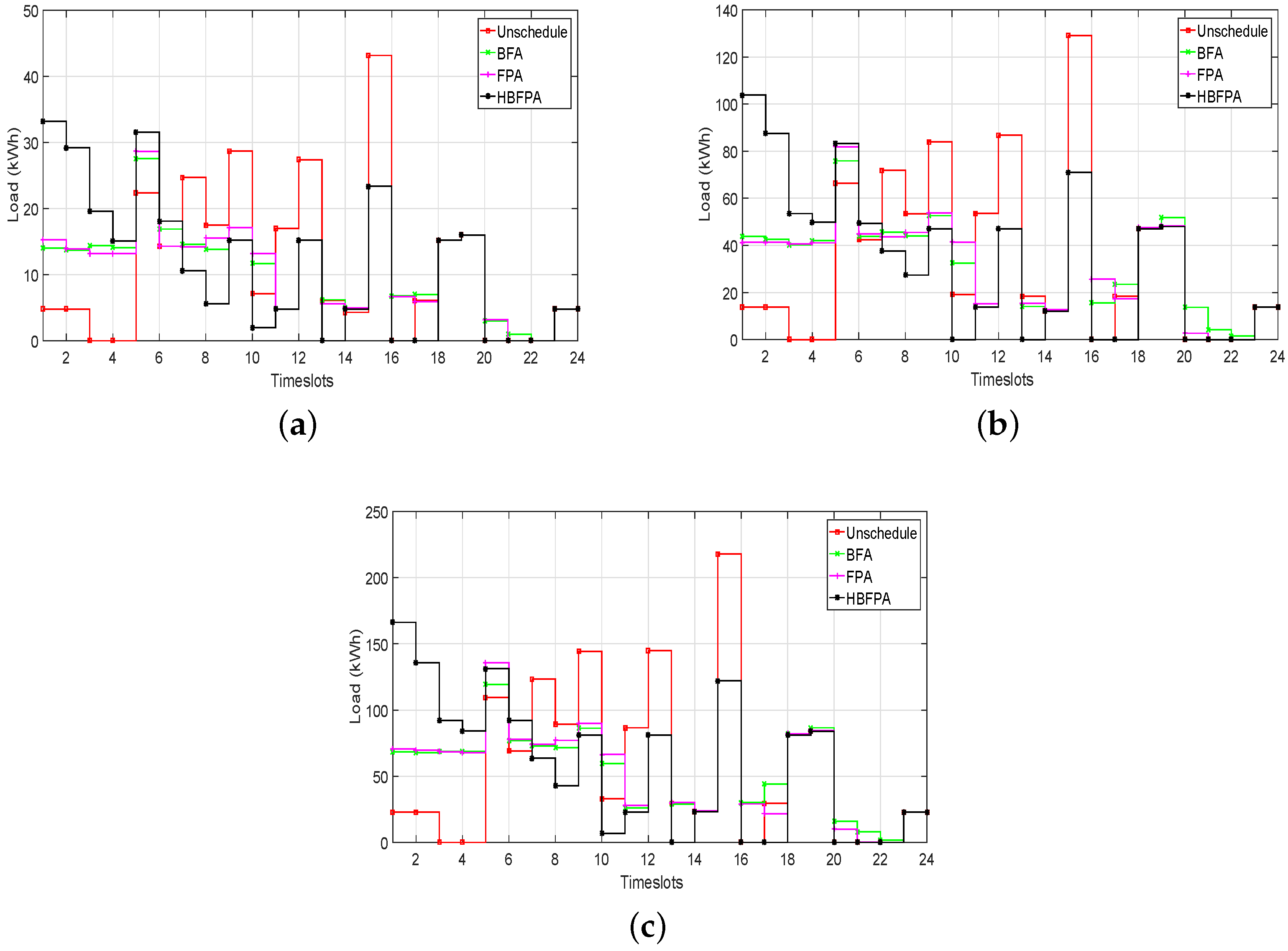
Figure 5.
Load for single home using real time pricing. (a) load using operational time interval of 1 min; (b) load using operational time interval of 20 min; (c) load using operational time interval of 30 min; (d) load using operational time interval of 60 min.
Figure 5.
Load for single home using real time pricing. (a) load using operational time interval of 1 min; (b) load using operational time interval of 20 min; (c) load using operational time interval of 30 min; (d) load using operational time interval of 60 min.
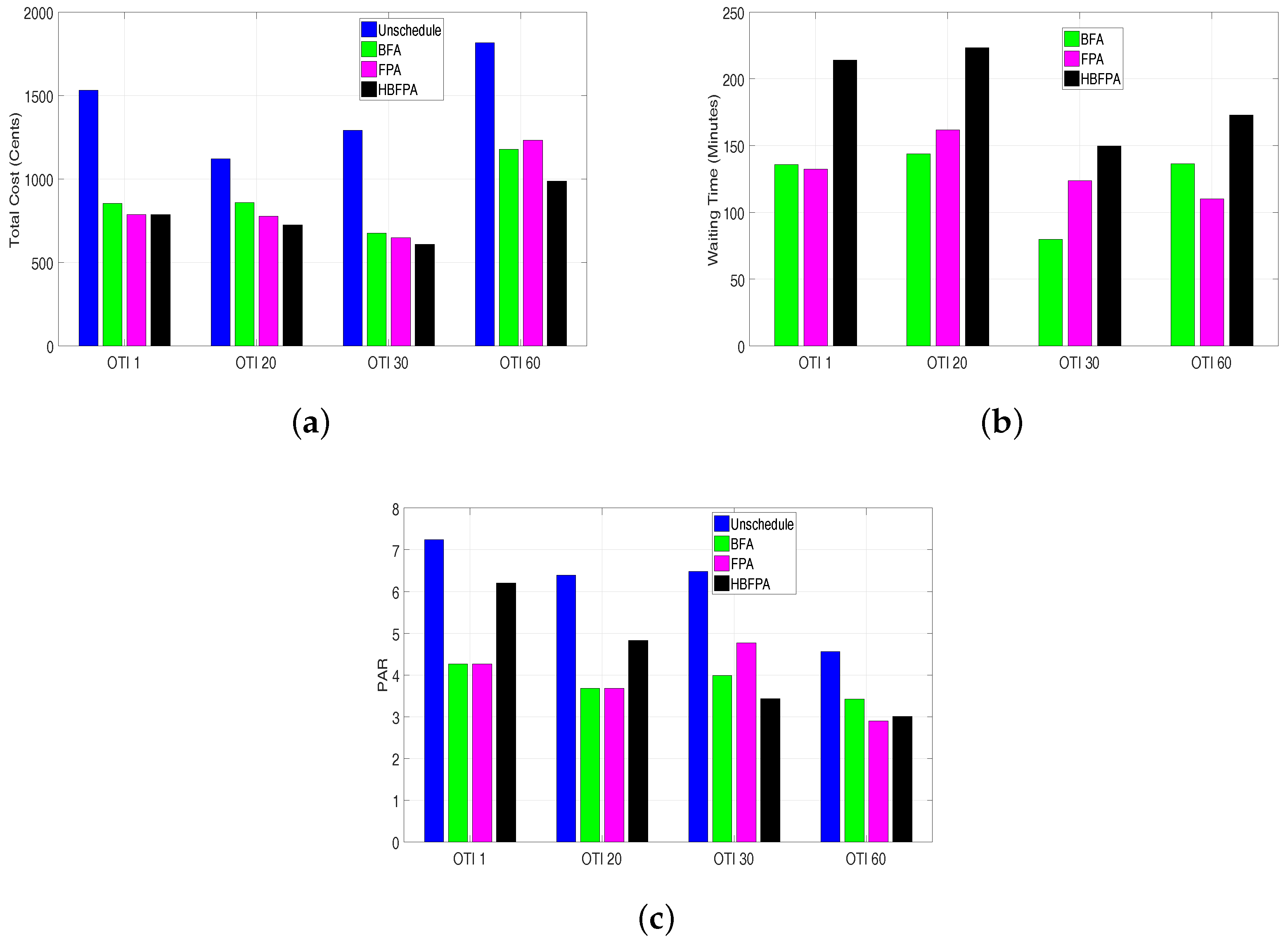
Figure 6.
Total cost, waiting time and peak to average ratio for a single home using critical peak pricing. (a) Electricity cost using operational time interval of 1, 20, 30, 60 min; (b) Waiting time using operational time interval of 1, 20, 30, 60 min; (c) Peak to average ratio using operational time interval of 1, 20, 30, 60 min.
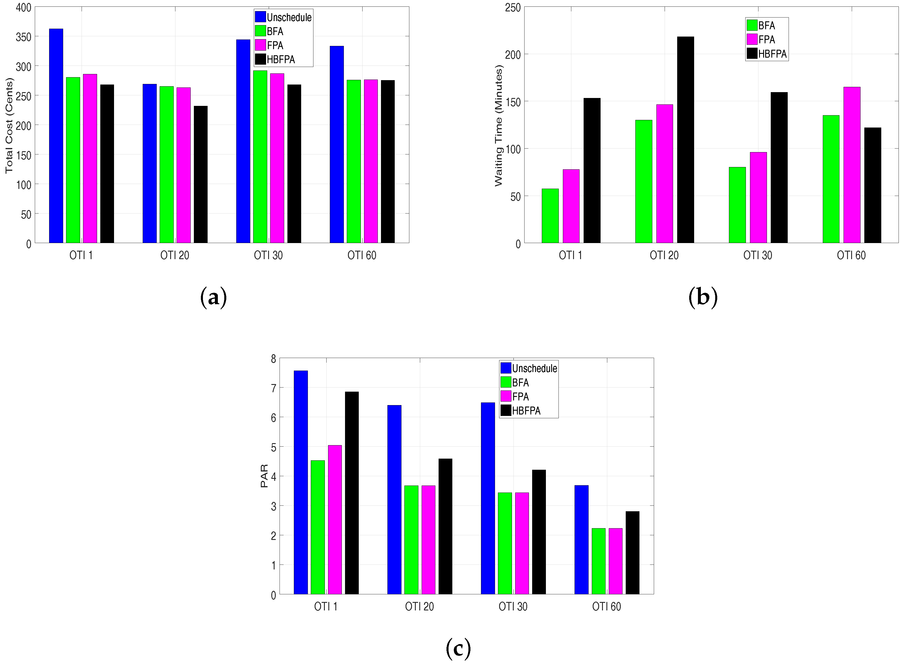
Figure 7.
Total cost, waiting time and peak to average ratio for single home using real time pricing. (a) Electricity cost using operational time interval of 1, 20, 30, 60 min; (b) Waiting time using operational time interval of 1, 20, 30, 60 min; (c) Peak to average ratio using operational time interval of 1, 20, 30, 60 min.
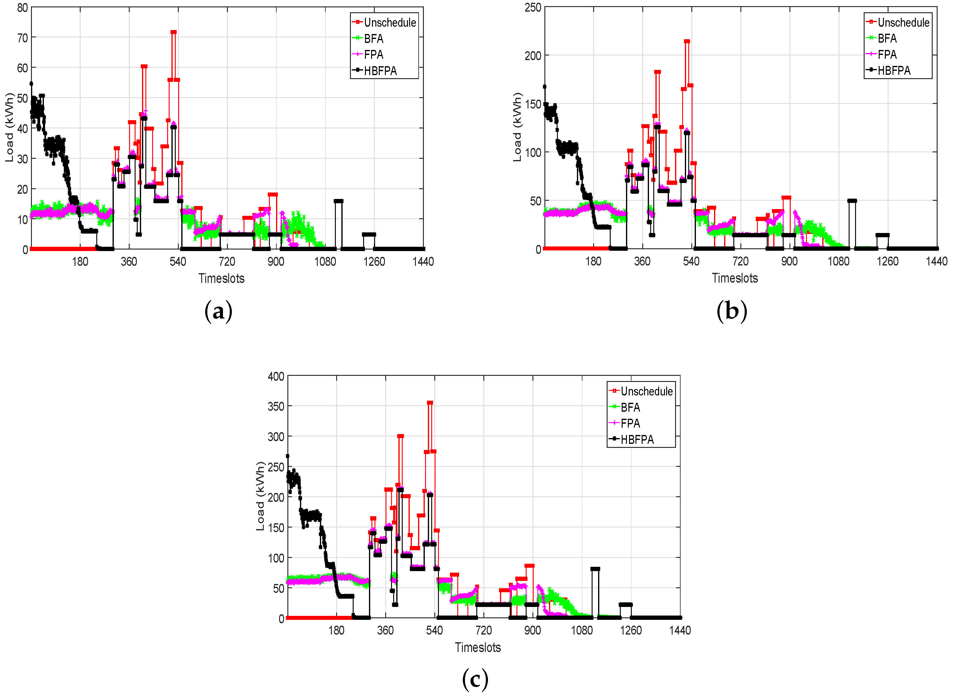
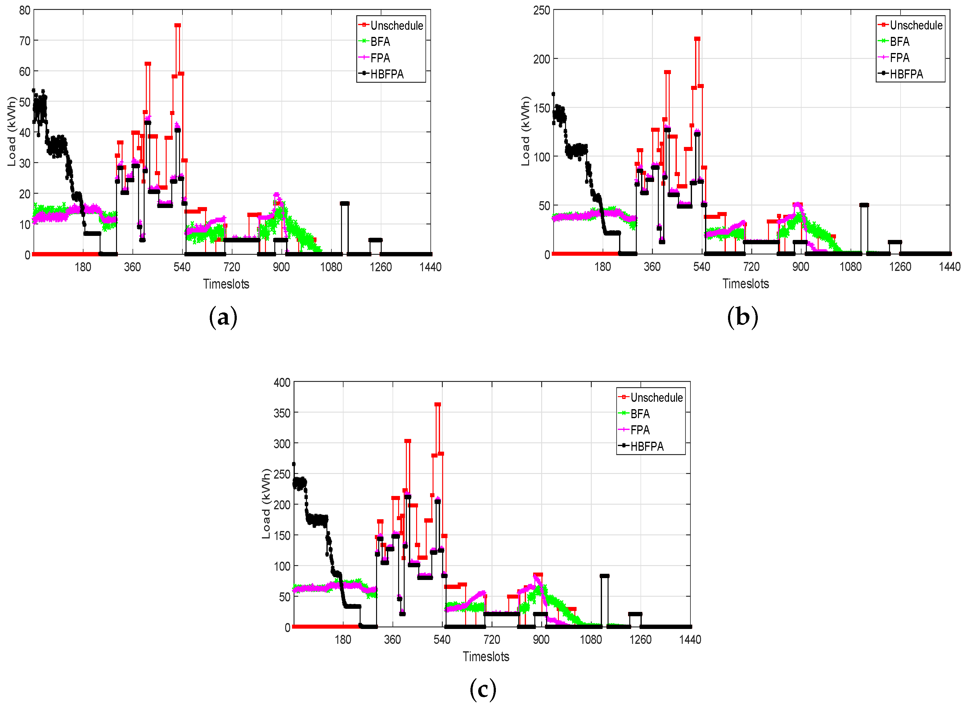
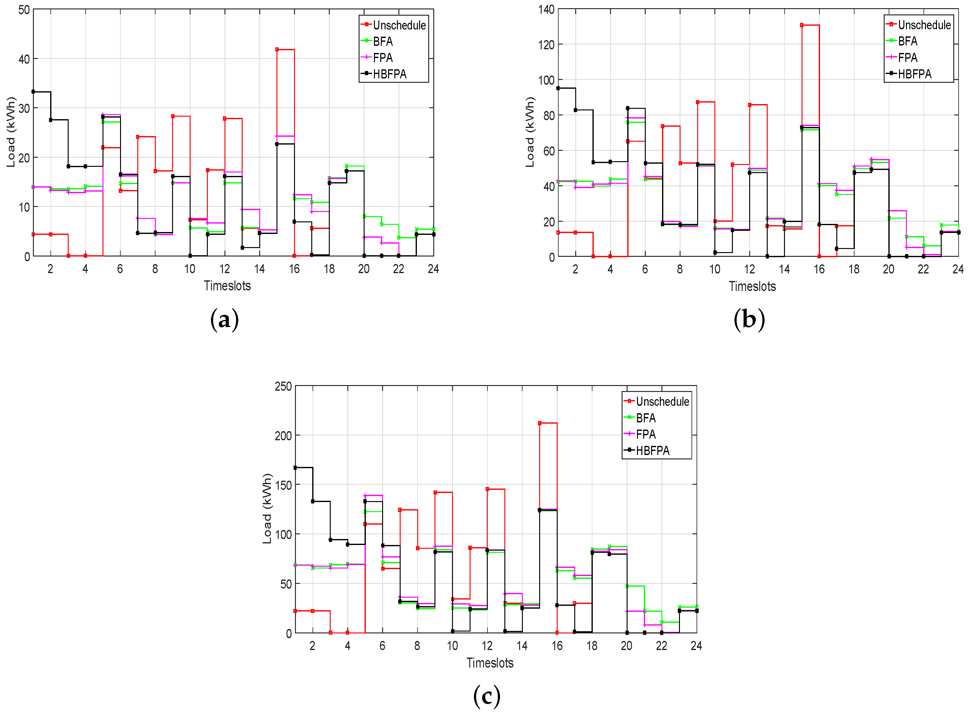
Figure 8.
Load for multiple homes: (10, 30 and 50) using critical peak pricing. (a) load using operational time interval of 1 min for 10 homes; (b) load using operational time interval of 1 min for 30 homes; (c) load using operational time interval of 1 min for 50 homes.
Figure 8.
Load for multiple homes: (10, 30 and 50) using critical peak pricing. (a) load using operational time interval of 1 min for 10 homes; (b) load using operational time interval of 1 min for 30 homes; (c) load using operational time interval of 1 min for 50 homes.
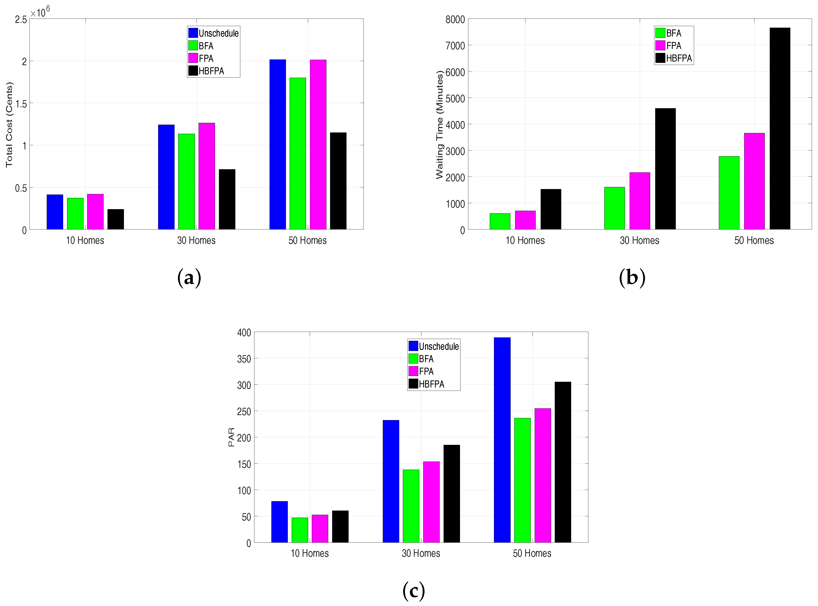
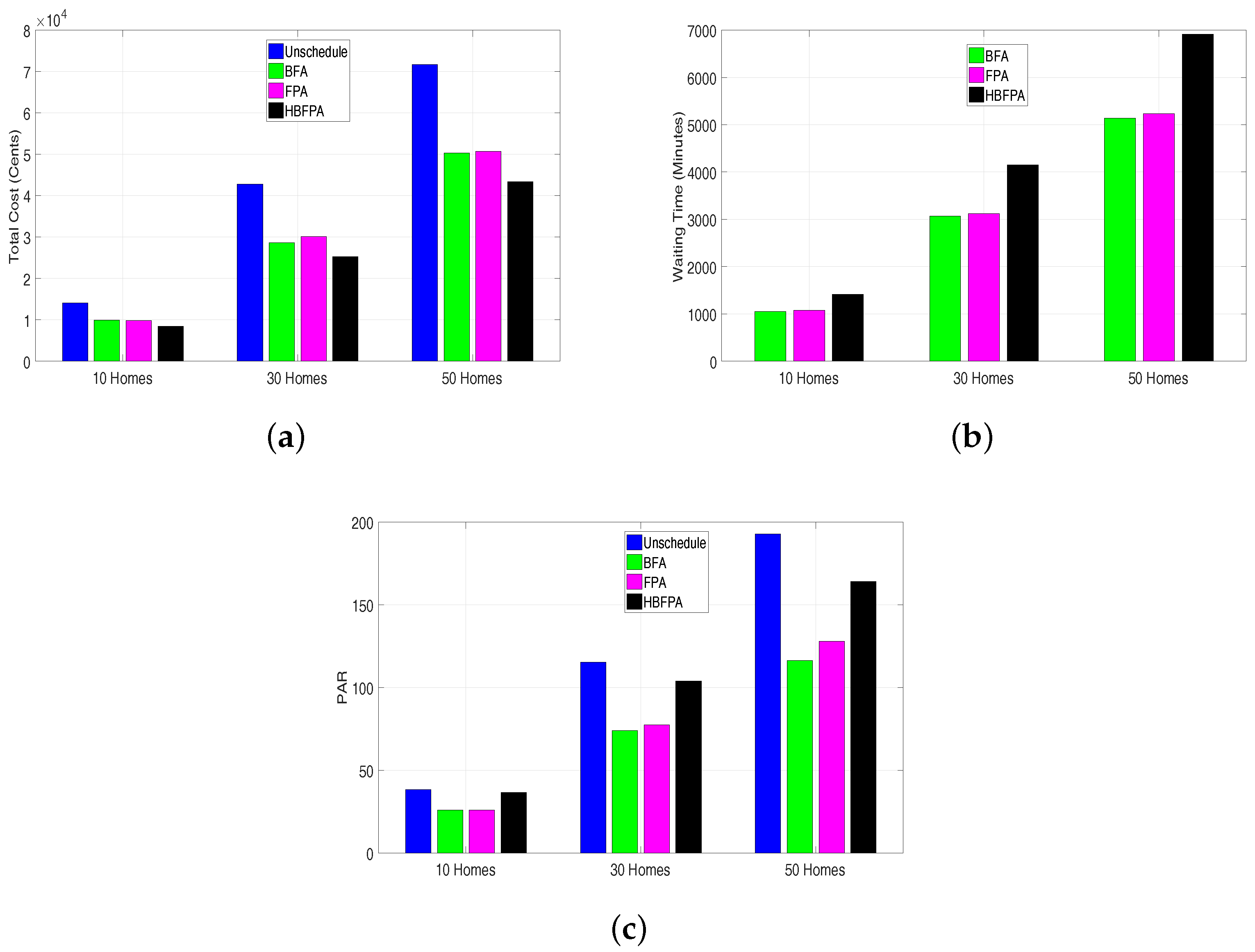
Figure 9.
Electricity cost, waiting time and peak to average ratio for multiple homes: (10, 30 and 50) using critical peak pricing. (a) Electricity cost using operational time interval of 1 min; (b) Waiting time using operational time interval of 1 min; (c) Peak to average ratio using operational time interval of 1 min.
Figure 10.
Load for multiple homes: (10, 30 and 50) using Real time pricing. (a) load using operational time interval of 1 min for 10 homes; (b) load using operational time interval of 1 min for 30 homes; (c) load using operational time interval of 1 min for 50 homes.
Figure 10.
Load for multiple homes: (10, 30 and 50) using Real time pricing. (a) load using operational time interval of 1 min for 10 homes; (b) load using operational time interval of 1 min for 30 homes; (c) load using operational time interval of 1 min for 50 homes.
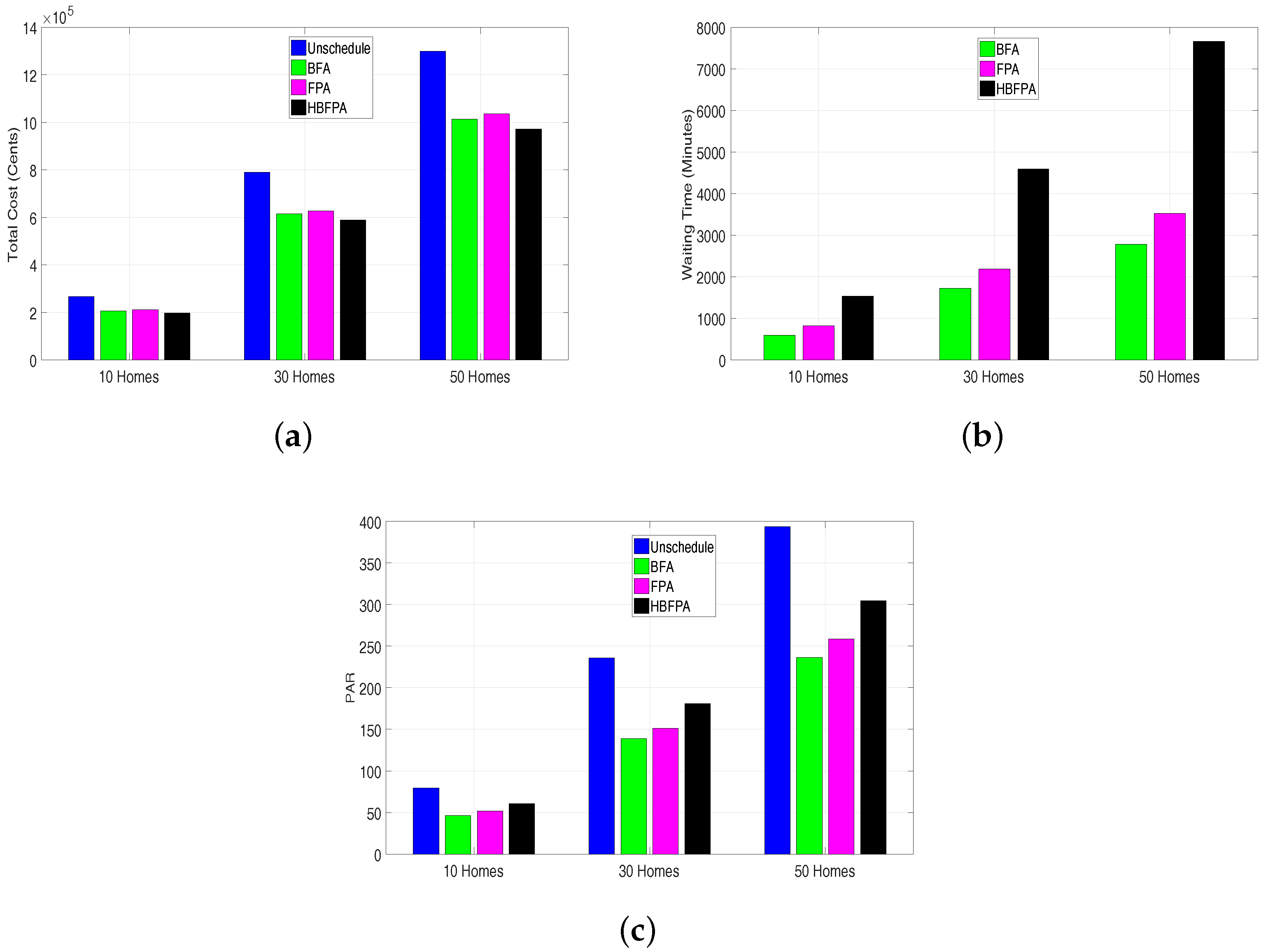
Figure 11.
Electricity cost, waiting time and peak to average ratio for multiple homes: (10, 30 and 50) using real time pricing. (a) Electricity cost using operational time interval of 1 min; (b) Waiting time using operational time interval of 1 min; (c) Peak to average ratio using operational time interval of 1 min.
Figure 12.
Load for multiple homes: (10, 30 and 50) using critical peak pricing. (a) load using operational time interval of 60 min for 10 homes; (b) load using operational time interval of 60 min for 30 homes; (c) load using operational time interval of 60 min for 50 homes.
Figure 12.
Load for multiple homes: (10, 30 and 50) using critical peak pricing. (a) load using operational time interval of 60 min for 10 homes; (b) load using operational time interval of 60 min for 30 homes; (c) load using operational time interval of 60 min for 50 homes.
Figure 13.
Electricity cost, waiting time and peak to average ratio for multiple homes: (10, 30 and 50) using critical peak pricing. (a) Electricity cost using operational time interval of 60 min; (b) Waiting time using operational time interval of 60 min; (c) Peak to average ratio using operational time interval of 60 min.
Figure 14.
Load for multiple homes: (10, 30 and 50) using real time pricing. (a) load using operational time interval of 60 min for 10 homes; (b) load using operational time interval of 60 min for 30 homes; (c) load using operational time interval of 60 min for 50 homes.
Figure 14.
Load for multiple homes: (10, 30 and 50) using real time pricing. (a) load using operational time interval of 60 min for 10 homes; (b) load using operational time interval of 60 min for 30 homes; (c) load using operational time interval of 60 min for 50 homes.
Figure 15.
Electricity cost, waiting time and peak to average ratio for multiple homes: (10, 30 and 50) using real time pricing. (a) Electricity cost using operational time interval of 60 min; (b) Waiting time using operational time interval of 60 min; (c) Peak to average ratio using operational time interval of 60 min.
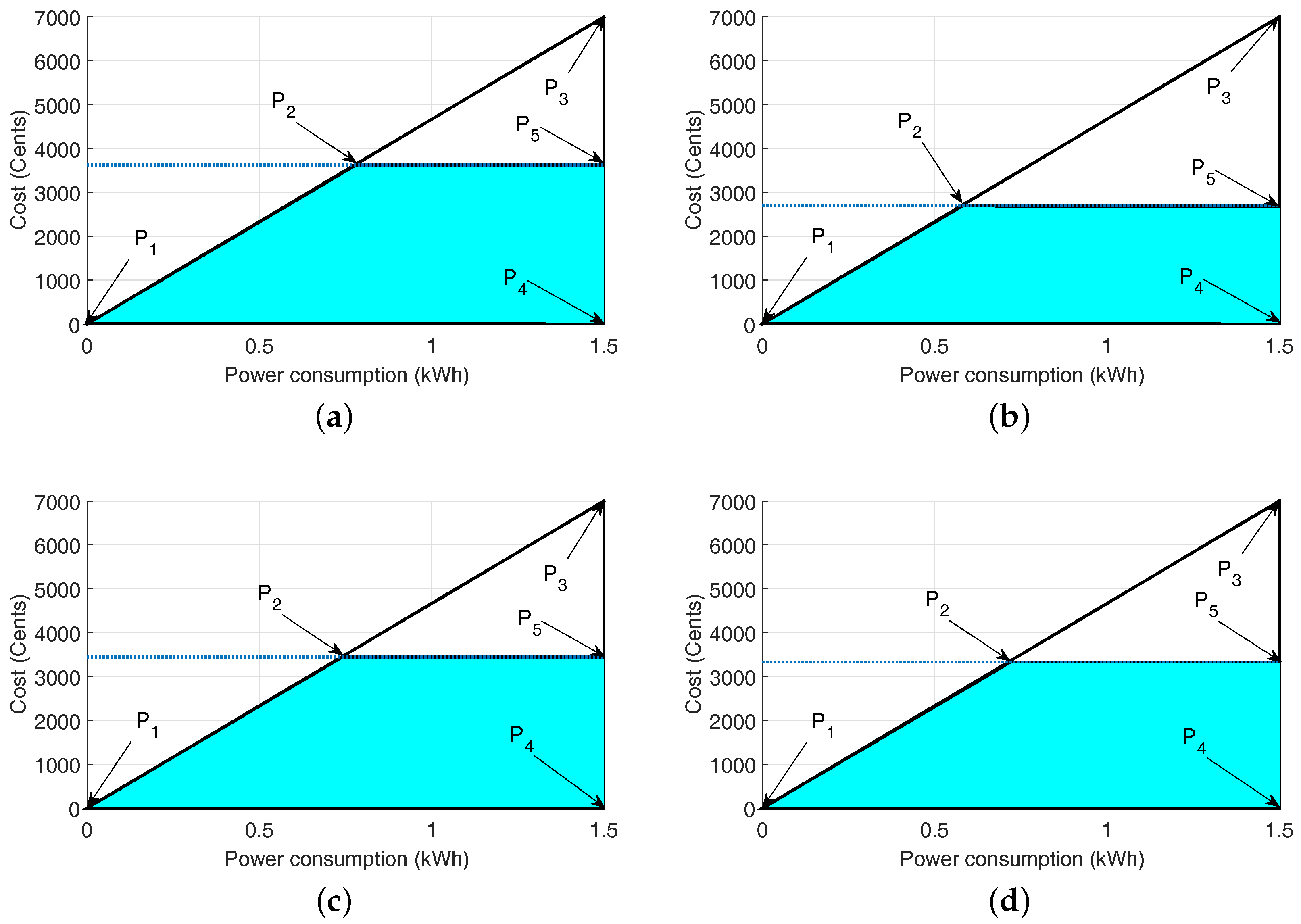
Figure 16.
Feasible regions for a single home using critical peak pricing. (a) Operational time interval of 1 min; (b) Operational time interval of 20 min; (c) Operational time interval of 30 min; (d) Operational time interval of 60 min.
Figure 16.
Feasible regions for a single home using critical peak pricing. (a) Operational time interval of 1 min; (b) Operational time interval of 20 min; (c) Operational time interval of 30 min; (d) Operational time interval of 60 min.
Figure 17.
Feasible regions for a single home using real time pricing. (a) Operational time interval of 1 min; (b) Operational time interval of 20 min; (c) Operational time interval of 30 min; (d) Operational time interval of 60 min.
Figure 17.
Feasible regions for a single home using real time pricing. (a) Operational time interval of 1 min; (b) Operational time interval of 20 min; (c) Operational time interval of 30 min; (d) Operational time interval of 60 min.
Table 1.
Summarized literature review.
Table 1.
Summarized literature review.
| Schemes | Achievement | Limitations |
|---|
| GA, BPSO, ACO [6] | Cost, PAR reduction and UC maximization | Computational complexity is not considered |
| BFOA, BFOA, GA, BPSO, WDO, GBPSO [7] | Reduces the EC and limits PAR | Trade-off between EC and PAR is not considered |
| GA, PSO, WDO, BFO, HGPSO [8] | Minimizes the electricity bill by | EC and PAR reduction are not considered |
| scheduling household appliances | |
| BFOA [9] | Reduces the EC with affordable UC | Trade-off among EC and |
| UC is not considered |
| BPSO [10] | Develops efficient scheme to minimize the EC | Privacy of user is not considered |
| MOEA [11] | EC minimization and reduction in WT | Consumer’s threshold limit is not focused |
| DR programs [13] | Minimize power consumption | Implements the DR program |
| peak demand hours not considered |
| BPSO [16] | Reduces peak hours demands | Peak demand is reduced |
| Reduction in the bill | Electric cost is not considered |
| HSA [17] | Reduces operational cost | UC is not considered |
| DSM model is presented using GA [18] | Reduces operational cost, PAR | Time complexity is completely ignored |
| In-place (PL) generalized algorithm [19] | EC and UC trade-off | Ignores the system complexity |
| GA | EC and PAR reduction | System complexity is ignored |
| current procedural terminology [20] | | |
| GA [21] | EC and PAR is minimized by the proposed scheme | Installation cost is completely ignored |
| GA [22] | EC is reduced by using GA | UC is ignored and PAR is also neglected |
| GA [23] | EC is minimized with reduction in PAR | UC is neglected |
| Hybrid algorithm using FPA and TS [24] | Hybrid version to optimize unconstrained problems | Ignores the optimization problem with multiple constrains |
| FPA [25] | Side lobe level minimization and null placement | Ignores interferences in undesired direction |
Table 2.
Terms used in equations and their notations.
Table 2.
Terms used in equations and their notations.
| Terms | Notations |
|---|
| Electric rate per slot (t) | |
| Power rating per appliance (ap) | |
| Maximum population size | |
| Appliance load | |
| Scheduled load | |
| Unscheduled L | |
| Domain of electric rate | |
| Fitness function | |
| Load per slot (t) | |
| Appliances | |
Table 3.
Power rating and length of operational time for operational time interval 20 min.
Table 3.
Power rating and length of operational time for operational time interval 20 min.
| Group | Appliances | PR (kWh) | LOTs |
|---|
| Controllable Appliances | Oven | 1.30 | 10.0 |
| Kettle | 2.00 | 1.00 |
| Coffee Maker | 0.80 | 4.00 |
| Rice Cooker | 0.85 | 2.00 |
| Blender | 0.30 | 2.00 |
| Frying Pan | 1.10 | 3.00 |
| Toaster | 0.90 | 1.00 |
| Fan | 0.20 | 15.0 |
| Shiftable appliances | Washing Machine | 0.50 | 6.00 |
| Clothes Dryer | 1.20 | 6.00 |
| Non-Shiftable Appliances | Dish Washer | 0.70 | 8.00 |
| Vacuum Cleaner | 0.40 | 8.00 |
| Hair Dryer | 1.50 | 2.00 |
| Iron | 1.00 | 6.00 |
Table 4.
Terms used in hybrid bacterial flower pollination algorithm and their notations.
Table 4.
Terms used in hybrid bacterial flower pollination algorithm and their notations.
| Terms | Notations |
|---|
| OTIs | t |
| Total time in hours | T |
| Upper bound | |
| Lower bound | |
| Appliances | D |
| Fitness | |
| Maximum population size | |
| Newly generated population | Xnew |
| Old generated population | X |
Table 5.
Electricity cost for 24 h (for single home).
Table 5.
Electricity cost for 24 h (for single home).
| Techniques | Cost (Cents) Using CPP | |
|---|
| 1 min | 20 min | 30 min | 60 min |
|---|
| Unscheduled | 1.5323 × | 1.1210 × | 1.2912 × | 1.1319 × |
| BFOA | 848.3800 | 829.7933 | 753.6100 | 952.7100 |
| FPA | 785.6600 | 777.5267 | 804.0100 | 1.0423 × |
| HBFPA | 785.6600 | 725.2600 | 608.0100 | 762.3100 |
Table 6.
Electricity cost for 24 h (For single home).
Table 6.
Electricity cost for 24 h (For single home).
| Techniques | Cost (Cents) Using RTP | |
|---|
| 1 min | 20 min | 30 min | 60 min |
|---|
| Unscheduled | 362.3626 | 269.1267 | 344.2463 | 333.1345 |
| BFOA | 280.0945 | 265.0310 | 291.4513 | 275.6915 |
| FPA | 286.3116 | 267.5580 | 300.4783 | 276.2255 |
| HBFPA | 267.9894 | 235.0647 | 269.3313 | 275.1495 |
Table 7.
Peak to average ratio for 24 h (for single homes).
Table 7.
Peak to average ratio for 24 h (for single homes).
| Techniques | PAR Using CPP | |
|---|
| 1 min | 20 min | 30 min | 60 min |
|---|
| Unscheduled | 7.241 | 4.9 | 3.47 | 3.3784 |
| BFOA | 3.4365 | 6.48 | 3.99 | 3.43 |
| FPA | 3.5248 | 3.68 | 2.22 | 2.2289 |
| HBFPA | 6.2047 | 4.4388 | 3.4657 | 3.2657 |
Table 8.
Peak to average ratio for 24 h (for single homes).
Table 8.
Peak to average ratio for 24 h (for single homes).
| Techniques | PAR Using RTP | |
|---|
| 1 min | 20 min | 30 min | 60 min |
|---|
| Unscheduled | 7.5619 | 6.3920 | 6.4850 | 3.6803 |
| BFOA | 4.5242 | 3.6784 | 3.8245 | 3.3175 |
| FPA | 5.4937 | 3.6784 | 3.4365 | 2.2289 |
| HBFPA | 6.2047 | 4.3417 | 4.2125 | 3.2138 |
Table 9.
Waiting time for 24 h (for single homes).
Table 9.
Waiting time for 24 h (for single homes).
| Techniques | Waiting Time Using CPP | |
|---|
| 1 min | 20 min | 30 min | 60 min |
|---|
| BFOA | 137.3321 | 154.1667 | 86.7857 | 139.2857 |
| FPA | 140.0812 | 153.3929 | 102.6786 | 147.8571 |
| HBFPA | 214.3473 | 227.5595 | 149.8214 | 135.00 |
Table 10.
Waiting time for 24 h (for single homes).
Table 10.
Waiting time for 24 h (for single homes).
| Techniques | Waiting Time Using RTP | |
|---|
| 1 min | 20 min | 30 min | 60 min |
|---|
| BFOA | 54.9940 | 130.9762 | 80.2500 | 133.5714 |
| FPA | 59.7152 | 147.9762 | 90.5357 | 165.00 |
| HBFPA | 153.5777 | 228.5714 | 160.1786 | 130.00 |
Table 11.
Random power ratings in (kWh).
Table 11.
Random power ratings in (kWh).
| Appliances | Power Rating 1 | Power Rating 2 | Power Rating 3 | Power Rating 4 |
|---|
| Washing-Machine | 0.50 | 0.70 | 0.90 | 0.40 |
| Clothes Dryer | 10.0 | 1.20 | 1.40 | 1.60 |
| Dish Washer | 0.38 | 0.50 | 0.70 | 0.80 |
| Vacuum Cleaner | 0.80 | 1.00 | 0.20 | 0.50 |
| Hair Dryer | 1.50 | 1.20 | 1.40 | 1.70 |
| Iron | 1.00 | 1.30 | 1.50 | 1.20 |
| Oven | 1.30 | 1.50 | 1.70 | 1.90 |
| Kettle | 2.00 | 2.15 | 2.40 | 2.14 |
| Coffee Maker | 0.80 | 0.40 | 0.50 | 0.20 |
| Rice Cooker | 0.85 | 0.89 | 0.72 | 0.79 |
| Blender | 0.30 | 0.47 | 0.40 | 0.70 |
| Frying Pan | 1.10 | 1.50 | 1.90 | 2.00 |
| Toaster | 0.90 | 1.00 | 0.50 | 0.70 |
| Fan | 0.20 | 0.50 | 0.40 | 0.70 |
Table 12.
Electricity cost for 24 h (for multiple homes).
Table 12.
Electricity cost for 24 h (for multiple homes).
| Techniques | Cost (Cents) Using CPP for OTI 1 min |
|---|
| 10 homes | 30 homes | 50 homes |
|---|
| Unscheduled | 4.2213 × | 1.2535 × | 2.1077 × |
| BFOA | 3.8669 × | 1.1425 × | 1.9247 × |
| FPA | 4.4563 × | 1.2881 × | 2.1096 × |
| HBFPA | 0.2128 × | 0.7098 × | 1.2205 × |
Table 13.
Waiting time for 24 h (for multiple homes).
Table 13.
Waiting time for 24 h (for multiple homes).
| Techniques | WT Using CPP for OTI 1 min |
|---|
| 10 homes | 30 homes | 50 homes |
|---|
| BFOA | 544.0428 | 1.7259 × | 2.8516 × |
| FPA | 722.7521 | 2.0134 × | 3.6380 × |
| HBFPA | 1.5302 × | 4.5947 × | 7.6534 × |
Table 14.
Peak to average ratio for 24 h (for multiple homes).
Table 14.
Peak to average ratio for 24 h (for multiple homes).
| Techniques | PAR Using CPP for OTI 1 min |
|---|
| 10 homes | 30 homes | 50 homes |
|---|
| Unscheduled | 75.9236 | 233.9259 | 381.1938 |
| BFOA | 46.1947 | 137.6369 | 231.5394 |
| FPA | 49.2012 | 150.6242 | 248.5587 |
| HBFPA | 61.5829 | 180.9010 | 304.4469 |
Table 15.
Electricity cost for 24 h (for multiple homes).
Table 15.
Electricity cost for 24 h (for multiple homes).
| Techniques | Cost (Cents) Using RTP for OTI 1 min |
|---|
| 10 homes | 30 homes | 50 homes |
|---|
| Unscheduled | 2.6912 × | 7.9680 × | 1.2990 × |
| BFOA | 2.0976 × | 6.2206 × | 1.0124 × |
| FPA | 2.1458 × | 6.3795 × | 1.0328 × |
| HBFPA | 2.0176 × | 5.9593 × | 9.7160 × |
Table 16.
Waiting time for 24 h (for multiple homes).
Table 16.
Waiting time for 24 h (for multiple homes).
| Techniques | WT Using RTP for OTI 1 min |
|---|
| 10 homes | 30 homes | 50 homes |
|---|
| BFOA | 574.6065 | 1.6632 × | 6.7364 × |
| FPA | 746.8147 | 2.1254 × | 4.5967 × |
| HBFPA | 2.7175 × | 3.6963 × | 7.6552 × |
Table 17.
Peak to average ratio for 24 h (for multiple homes).
Table 17.
Peak to average ratio for 24 h (for multiple homes).
| Techniques | PAR Using RTP for OTI 1 min |
|---|
| 10 homes | 30 homes | 50 homes |
|---|
| Unscheduled | 77.0644 | 232.1643 | 394.5380 |
| BFOA | 45.6238 | 138.9392 | 234.6092 |
| FPA | 50.2105 | 153.5715 | 253.3993 |
| HBFPA | 57.1704 | 184.7282 | 302.1077 |
Table 18.
Electricity cost for 24 h (for multiple homes).
Table 18.
Electricity cost for 24 h (for multiple homes).
| Techniques | Cost (Cents) Using CPP for OTI 60 min |
|---|
| 10 homes | 30 homes | 50 homes |
|---|
| Unscheduled | 1.5059 × | 4.2003 × | 7.1746 × |
| BFOA | 1.0666 × | 2.9568 × | 4.9553 × |
| FPA | 1.0836 × | 2.9822 × | 5.1076 × |
| HBFPA | 0.83 × | 2.5075 × | 4.274 × |
Table 19.
Waiting time for 24 h (for multiple homes).
Table 19.
Waiting time for 24 h (for multiple homes).
| Techniques | WT Using CPP for OTI 60 min |
|---|
| 10 homes | 30 homes | 50 homes |
|---|
| BFOA | 1.0043 × | 3.2093 × | 5.1507 × |
| FPA | 1.0757 × | 3.2429 × | 4.1714 × |
| HBFPA | 1.3836 × | 4.1714 × | 6.8836 × |
Table 20.
Peak to average ratio for 24 h (for multiple homes).
Table 20.
Peak to average ratio for 24 h (for multiple homes).
| Techniques | PAR Using CPP for OTI 60 min |
|---|
| 10 homes | 30 homes | 50 homes |
|---|
| Unscheduled | 38.7901 | 112.7401 | 189.7837 |
| BFOA | 23.5727 | 78.1047 | 120.4385 |
| FPA | 24.6797 | 75.6910 | 129.6416 |
| HBFPA | 30.3457 | 98.0471 | 167.4858 |
Table 21.
Electricity cost for 24 h (for multiple homes).
Table 21.
Electricity cost for 24 h (for multiple homes).
| Techniques | Cost (Cents) Using RTP for OTI 60 min |
|---|
| 10 homes | 30 homes | 50 homes |
|---|
| Unscheduled | 3.9954 × | 1.2170 × | 2.0437 × |
| BFOA | 3.1541 × | 9.6811 × | 1.6242 × |
| FPA | 3.1884 × | 9.8798 × | 1.6251 × |
| HBFPA | 3.1877 × | 1.6242 × | 1.6039 × |
Table 22.
Waiting time for 24 h (for multiple homes).
Table 22.
Waiting time for 24 h (for multiple homes).
| Techniques | WT Using RTP for OTI 60 min |
|---|
| 10 homes | 30 homes | 50 homes |
|---|
| BFOA | 1.4314 × | 4.0729 × | 6.7364 × |
| FPA | 1.4371 × | 3.8336 × | 6.869 × |
| HBFPA | 1.3964 × | 4.1579 × | 6.9236 × |
Table 23.
Peak to average ratio for 24 h (for multiple homes).
Table 23.
Peak to average ratio for 24 h (for multiple homes).
| Techniques | PAR Using RTP for OTI 60 min |
|---|
| 10 homes | 30 homes | 50 homes |
|---|
| Unscheduled | 37.3187 | 115.6367 | 195.2858 |
| BFOA | 25.9190 | 74.4312 | 122.2942 |
| FPA | 25.8770 | 80.9041 | 129.3206 |
| HBFPA | 33.8192 | 102.8952 | 166.9638 |

 ,
, 


