Energy-Efficiency Performance Analysis and Maximization Using Wireless Energy Harvesting in Wireless Sensor Networks

Abstract

Paradigm shift to wireless power transfer provides opportunities for ultra-low-power devices to increase energy storage from electromagnetic (EM) sources. The notable gain occurs when EM sources deliver information as a meaningful signal with power transfer. Thus, energy harvesting (EH) is an active approach to obtain power from surrounding EM sources that transfer energy deliberately. This paper discusses energy efficiency (EE) trade-offs and EE maximization in simultaneous wireless power and information transfer (SWIPT) for wireless sensor networks (WSNs). The power splitting (PS) and time switching (TS) model for SWIPT are investigated in detail, where EE optimization is essential. This work formulates EE maximization problem as non-linear fractional programming and proposes a novel algorithm to solve the maximization problem using Lagrange dual decomposition. Numerical results reveal that the proposed algorithm maximizes EE in both PS and TS modes through noteworthy improvements.

1. Introduction

The next generation of wireless technology is growing and concurrently demand for power consumption is increasing. The wireless power transfer (WPT) has become a reality, and mainly has two approaches: One is magnetically coupled resonance, and the other is radio-frequency (RF) waveforms for power transfer [1]. The application of resonance coupling has some weaknesses in particular scenarios where mobile nodes cannot migrate. However, RF signal travels freely through the air and provides a real opportunity for mobility. Compared to coupled magnetic resonance, the RF signal is considered as a promising energy source for WPT. At present, there are a lot of interests in energy harvesting (EH) and a promising solution to recharge ultra-low-power devices [2,3].

Recently, simultaneous wireless information and power transfer (SWIPT) has increased its popularity in modern wireless networks. Several studies have considered SWIPT configuration in different modes such as power splitting (PS), time switching (TS), antenna switching (AS), and separated receiver architectures [4,5,6,7]. The combined study, where SWIPT concerns multiple inputs multiple outputs (MIMO) broadcast operations, is considered to identify its achievable rate-energy (RE) regions for PS and TS mode at the design level [8]. The SWIPT system based on secured orthogonal frequency division multiplexing (OFDM) is studied with wireless powered jammer for optimal power allocation [9], where the joint power allocation of jammer and transmitter is optimized to increase the secrecy rate and satisfy the EH constraint. The SWIPT deals with a multi-relay assisted two-hop cooperative communication [10], where each relay uses a PS protocol to settle the received signal energy for information decoding (ID) and EH. A SWIPT-aware fog computing investigated [11], where the sensor node performs EH and ID operations from a hybrid access point (HAP) through PS receiver architecture. On the other hand, Reference [12] investigates the SWIPT architecture which uses distinct peak-to-average-power-ratio (PAPR) for information and multi-sine waveforms for energy. In this case, the information conveys on different PAPR streams, which can be measured at the output of rectifier for EH, and permits a low-energy combined receiver. In [13,14,15,16,17], the combined power control and time allocation is considered to examine the relationship between energy efficiency (EE) and delay concerning in wireless powered communication network (WPCN). The future trends in WPT applications focused on wireless networks, the concept of joint interest is introduced [18], where the physical and energy-aware properties in clustering and resource management processes support various internet of things applications. A cognitive radio network based on multiuser SWIPT is investigated [19] and an efficient weighted sum harvested energy (WSHE) algorithm is proposed to find the optimal beamforming and PS ratios. Recently, Reference [20] introduces an energy-efficient distributed antenna system which uses the PS scheme at IoT device for EH and ID operations, by varying transmit power of allocated antenna port of IoT device. At present, the study on SWIPT focuses on cornering its basic architectural design and applications in some systems, such as MIMO wireless broadcast systems and cooperative relay network. In energy-constrained wireless technology, EE maximization aspect is not considered in detail for PS and TS mode. This work formulates EE maximization problem as non-linear fractional programming and proposes a novel algorithm to solve the maximization problem using Lagrange dual decomposition. By utilizing the SWIPT system model, this work adapts two different receiver’s architectures for PS and TS mode. The EE is enhanced notably by modifying PS ratio of power splitter as well as varying time-slots.

The rest of this paper is organized as follows. Section 2 begins with introducing the SWIPT system model. Section 3 formulates the non-convex optimization problem in PS and TS modes, and proposes iterative algorithms for optimal solutions. Numerical results are presented in Section 4, followed by conclusions in Section 5.

2. System Model

2.1. Simultaneous Wireless Information and Power Transfer (SWIPT)

The system performance can be predicted by using system-level simulation (SLS), which gives benefits of modifying simulation parameters with low cost and risk [21]. In SWIPT, the receiver not particularly gains energy as a conventional receiver but also harvests energy from the incoming RF signal [22,23,24,25]. The receiver is used for mainly two purposes: one is EH, and the other is for ID as shown in Figure 1. The system model consists of a transmitter (Tx) and receiver (Rx) antenna, where EH and ID functions are performed using the co-located antenna at the receiver. Whereas, the transmitter contains x (t)signal with a constant transmit power $P_T$, exhibits amount of energy and coded information to the receiver over a quasi-static fading channel. And $n(t)$ and $h_o$ denotes the noise and channel gain respectively.

$$\begin{array}{c}\hfill y(t)=h_o\sqrt{P_T}x(t)+n(t).\end{array}$$

(1)

2.2. Energy Efficiency in Power Splitting Mode

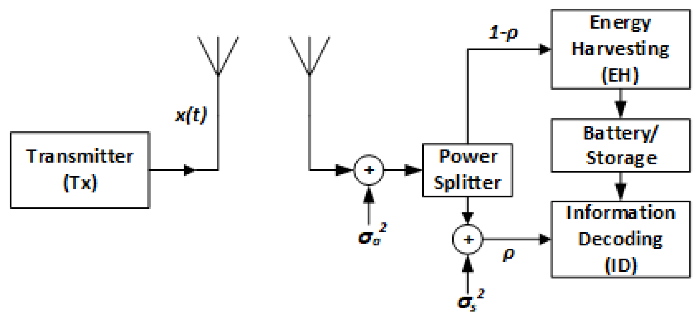
In the RF field, straightforward implementation of EH destroys the information contents [26] and to avoid such a situation the incoming signal needs to split. In Figure 2 for successful energy transfer, the signal divides into two power streams at the receiver: One is for EH and the other is for ID. For such case, $\rho$ is used as PS ratio between EH and ID, ranges from 0 to 1. In (2) and (3), $\rho$ and $1-\rho$ are the ratios designated for ID and EH functions, respectively. The $Q_{EH}$ represents the power of harvest energy at the receiver and $\xi$ is the EH efficiency. Equation (3) represents the information rate, where B is the total transmission bandwidth, and $N_o$ is the sum of the antenna noise ${\sigma }_a^2$ and signal power noise ${\sigma }_s^2$. In PS mode, ${\eta }_{EE}$ is defined as a ratio of total information rate R and total power consumption $E_T$ [23]. Whereas, h represents the channel power gain, equals to $|h_o{|}^2$. $P_c$ and $P_T$ are circuit power conversion and transmit power, respectively. And $\mu$ is the inverse power amplifier efficiency. By substituting R and $E_T$ in (4), we get ${\eta }_{EE}$, where B denotes channel bandwidth, as below

$$\begin{array}{c}\hfill Q_{EH}=\xi h{P}_T(1-\rho ),\end{array}$$

(2)

$$\begin{array}{c}\hfill R=B{\log }_2(1+\frac{\rho h{P}_T}{N_o}),\end{array}$$

(3)

$$\begin{array}{c}\hfill {\eta }_{EE}={\displaystyle \frac{B{\log }_2(1+\frac{\rho h{P}_T}{N_o})}{P_c+\mu P_T-\xi h{P}_T(1-\rho )}}.\end{array}$$

(4)

2.3. Energy Efficiency in Time Switching Mode

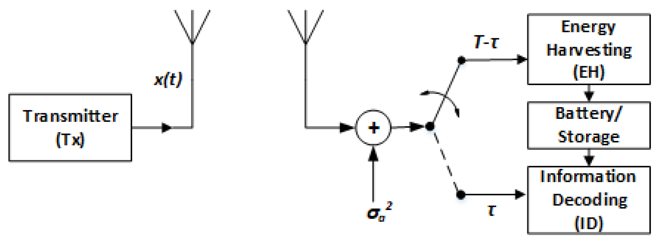
In the TS mode, time switching is performed by varying time slots for EH and ID operations. In Figure 3, received signal switches time between EH and ID at the receiver. The additional time for downlink results in more harvested energy for the receiver and fewer time slots slows the transmission for uplink data. In this mode, $\tau$ represents a switching ratio between EH and ID, which ranges $[\tau ,T]$. In (5) and (6), $T-\tau$ and $\tau$ are allocated for EH and ID operations, respectively. Equation (6) represents the information rate, where ${\sigma }_a^2$ is the antenna noise at the receiver. For the TS mode, ${\eta }_{EE}$ can be express as

$$\begin{array}{c}\hfill Q_{EH}=\xi h{P}_T(T-\tau ),\end{array}$$

(5)

$$\begin{array}{c}\hfill R=B{\log }_2(1+\frac{h{P}_T}{{\sigma }_a^2})\tau ,\end{array}$$

(6)

$$\begin{array}{c}\hfill {\eta }_{EE}={\displaystyle \frac{B{\log }_2(1+\frac{h{P}_T}{{\sigma }_a^2})\tau }{T(P_c+\mu P_T)-\xi h{P}_T(T-\tau )}}.\end{array}$$

(7)

3. Problem Formulation

3.1. Energy Efficiency Maximization in Power Splitting Mode

For successful information transmission, ID rate and a total amount of power harvested from RF signal must be more than or equal to $R_{min}$ and $E_{min}$, respectively. The splitting ratio $\rho$ is between 0 and 1, where $P_T$ ranges from 0 to maximum transmit power $P_{th}$. Then, maximization problem can be written as

$$\begin{array}{c}\hfill \underset{P_T,\rho }{\max }{\eta }_{EE}\end{array}$$

(8)

$$\begin{array}{cc}\hfill \mathit{subject}\mathit{to}& \hfill R\ge R_{min},\end{array}$$

(9)

$$\begin{array}{c}\hfill E_T\ge E_{min},\end{array}$$

(10)

$$\begin{array}{c}\hfill P_T\le P_{th},\end{array}$$

(11)

$$\begin{array}{c}\hfill 0\le P_T,\end{array}$$

(12)

$$\begin{array}{c}\hfill 0\le \rho \le 1.\end{array}$$

(13)

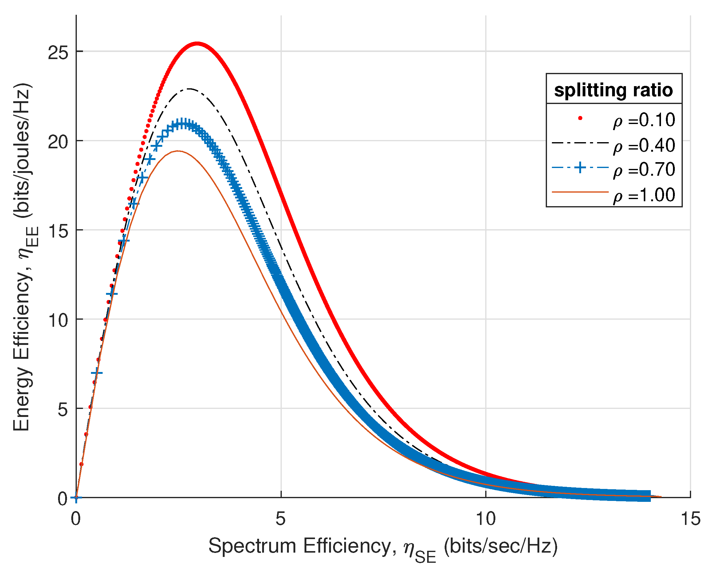
Spectral efficiency ${\eta }_{SE}$ is defined as the ratio of information rate to the total bandwidth of the channel. From this relationship, we can obtain the transmit power. Substituting $P_T$ into (7) gives EE vs. SE trade-off for PS mode shown in (14). By using this relationship, as a result, a quasi-concave shape is represented in Figure 4, for different PS ratios. The available channel bandwidth is 150 MHz, $P_T$ ranges from 10 to 40 mW, and the circuit power conversion $P_c$ is 10 mW at the receiver. For simplicity, $\xi$ and h are set to 1; and ${\sigma }_a^2$ and ${\sigma }_S^2$ are equal to $-20$ dBm. It is worth noting that, initially, EE increases to peak value while SE increases. After attaining peak value, EE decreases with respect to defined parameters resulting in quasi-concave shape [7].

$${\eta }_{EE}=\frac{Bh\rho ({\eta }_{SE})}{h\rho P_c+(\mu -h\xi -\rho h\xi )(2^{{\eta }_{SE}}-1)N_o}.$$

(14)

Lemma 1.

For PS ratio ρ, the objective function of EE is quasi-concave with respect to $P_T$. By using transmit power in PS mode, the objective function of EE is also quasi-concave with respect to ρ.

Proof. 

After calculating first order condition (FOC) and second order condition (SOC), one can get

$$\begin{array}{c}\hfill \frac{{\partial }^{2}R}{{\partial }^2{P}_T}=-\frac{B{h}^2{\rho }^2}{ln2\ast {(N_o+h\rho P_T)}^2}<0,\end{array}$$

(15)

$$\begin{array}{c}\hfill \frac{{\partial }^{2}R}{{\partial }^2\rho }=-\frac{Bh{\sigma }_s^2{P}_T({\sigma }_s^{2}Y+2\rho {\sigma }_a^{2}Y)}{ln2\ast N_o^2{(N_o+\rho P_{T}h)}^2}<0.\end{array}$$

(16)

From (15), one can observe that second-order partial derivative of R with respect to the $P_T$ is concave. And in (16), R is concave with respect to the $\rho$ with the fact that $Y={\sigma }_a^2+P_{T}h$. In (2), EH is positive affine functions with respect to $P_T$. In (4), transmit power is a positive affine function with respect to $\rho$. From these observations, function ${\eta }_{EE}=R/E_T$ is the ratio between concave and affine function, and as a result, the output is a quasi-concave function. □

3.2. Energy Efficiency Maximization in Time Switching Mode

Similarly, for active communication in the TS mode, information rate must be more than or equal to $R_{min}$. The total amount of power must be more than or equals to $E_{min}$. The time switching constraint in TS mode ranges between $\tau$ and T. In addition, $P_T$ ranges from 0 to maximum transmit power $P_{th}$. Then the maximization problem can be written as

$$\begin{array}{c}\hfill \underset{P_T,\tau }{\max }{\eta }_{EE}\end{array}$$

(17)

$$\begin{array}{cc}\hfill \mathit{subject}\mathit{to}& \hfill R\ge R_{min},\end{array}$$

(18)

$$\begin{array}{c}\hfill E_T\ge E_{min},\end{array}$$

(19)

$$\begin{array}{c}\hfill P_T\le P_{th},\end{array}$$

(20)

$$\begin{array}{c}\hfill 0\le P_T,\end{array}$$

(21)

$$\begin{array}{c}\hfill 0\le \tau ,\end{array}$$

(22)

$$\begin{array}{c}\hfill \tau \le T.\end{array}$$

(23)

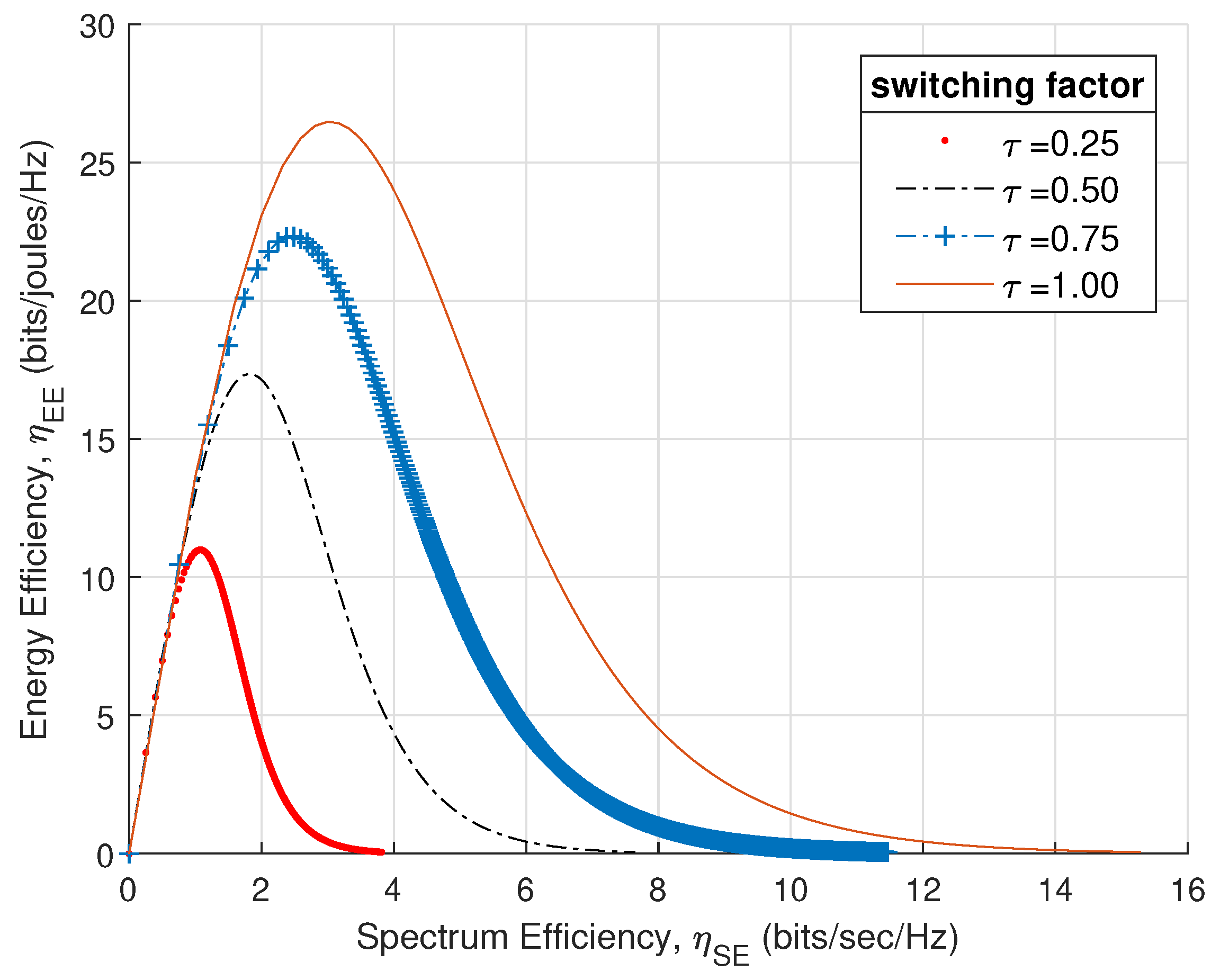
By using (24), the relationship between EE and SE, as shown in Figure 5, shows that EE initially increases to its peak value as SE increases. After attaining its peak value, EE decreases with respect to defined parameters resulting in quasi-concave shape [7].

$$\begin{array}{c}\hfill {\eta }_{EE}=\frac{Bh({\eta }_{SE})}{hT{P}_c+(T\mu -(T-\tau )h\xi )(2^{{\eta }_{SE}/\tau }-1)({\sigma }_a^2)}.\end{array}$$

(24)

Lemma 2.

For the switching ratio τ in TS mode, the objective function of EE is quasi-concave with respect to $P_T$. By using transmit power $P_T$ in TS mode, the objective function of EE is quasi-concave with respect to τ.

Proof. 

After calculating FOC and SOC, one can get

$$\begin{array}{c}\hfill \frac{{\partial }^{2}R}{{\partial }^2{P}_T}=-\frac{B{h}^2{\tau }^2}{ln2\ast Y^2}<0,\end{array}$$

(25)

$$\begin{array}{c}\hfill \frac{{\partial }^2{\eta }_{EE}}{{\partial }^2\tau }=-\frac{2BT{\log }_2(1+\frac{P_{T}h}{{\sigma }_a^2})\tau (P_c+\mu P_T-\xi P_{T}h)}{{[\xi P_{T}h\tau +T(P_c+\mu P_T-\xi P_{T}h)]}^3}<0.\end{array}$$

(26)

From (25), one can observe that second-order partial derivative of information rate R with respect to the $P_T$ is concave. In (2), EH is affine positive with respect to $P_T$. Furthermore, harvested energy is an affine positive function with respect to $\tau$ in (6), as result output is a quasi-concave function. Note that EE maximization problem in TS mode is concave-convex optimization problem and information rate R with respect to $\tau$ is concave. On the other hand, $E_T$ positive affine function with respect to $\tau$. From these observations, function ${\eta }_{EE}=R/E_T$ is the ratio between concave and affine function, and as a result, the output is a quasi-concave function. □

By using (26), variation with respect to $\tau$ is shown in Figure 5. From Lemmas 1 and 2, our objective function $({\eta }_{EE}=R/E_T)$, is the ratio of concave and affine function, in results, the output is a quasi-concave function. In the above lemmas, quasi-concavity and concavity of the objective function are revealed.

3.3. Optimal Solution of Power Splitting Mode

For the fractional problem for PS mode, the Dinkelbach’s method (i.e., Algorithm 1) can be used. Based on the Dinkelbach’s algorithm, this work proposes Algorithms 2 and 3 for PS and TS mode, respectively.

Algorithm 1: Dinkelbach’s algorithm

1   Initialization:$ϵ>0,i=0$ 2   ${\lambda }_i=0$ 3   while ($\mathit{mod}(F({\lambda }_i)>ϵ)$) do 4      $x=f(x)-{\lambda }_{i}h(x)$; 5      $F({\lambda }_i)=f(x_i)-{\lambda }_{i}h(x)$; 6      ${\lambda }_{i+1}=f(x_i)/h(x_i)$; 7      $i=i+1;$ 8   endwhile

Algorithm 2: Proposed iterative power splitting algorithm

1   Initialization: input parameters   2   ${\eta }_{EE}=0$ and $j=0$   3   while ($\mathit{mod}({\eta }_{EE}^j-{\eta }_{EE}^{j+1}>ϵ)$) do   4      $i=0;$   5      while ($({\eta }_{EE}^i-{\eta }_{EE}^{i+1}>ϵ,({\lambda }_1^{i+1}-{\lambda }_1^i,{\lambda }_2^{i+1}-{\lambda }_2^i,{\lambda }_3^{i+1}-{\lambda }_3^i)<ϵ)$) do   6         $i=i+1$;   7         Calculate optimal value of $P_T$   8         Calculate optimal value of $\rho$   9         Update: ${\lambda }_1^{i+1}=a_1(P_{max}-P_T)+{\lambda }_1^i$; 10         Update: ${\lambda }_2^{i+1}=a_2(E_T-E_{min})+{\lambda }_2^i$; 11         Update: ${\lambda }_3^{i+1}=a_3(R-R_{min})+{\lambda }_3^i$; 12      endwhile 13      By using $P_T^j\ast$ and ${\rho }^j\ast$, calculate optimal value of ${\eta }_{EE}^j\ast$ 14      $j=j+1;$ 15   endwhile

The main purpose of applying Dinkelbach’s method is to transform the concave-convex fractional problem (CCFP) into a convex optimization problem. To achieve an optimal solution in (8), Lagrangian dual decomposition is applied,

$$\begin{array}{c}\hfill \mathsf{\Lambda }(P_T,\rho ,{\lambda }_1,{\lambda }_2,{\lambda }_3)=R-{\eta }_{EE}{E}_T+{\lambda }_1(P_{th}-P_T)+{\lambda }_2(E_T-E_{min})+{\lambda }_3(R-R_{min}).\end{array}$$

(27)

The Lagrange multipliers ${\lambda }_1$, ${\lambda }_2$, and ${\lambda }_3$ are used for $P_T$, $R_{min}$, and $E_T$, respectively. For simplicity, we express

$$\begin{array}{c}\hfill W=P_{t}h\rho +N_o,\end{array}$$

(28)

$$\begin{array}{c}\hfill X={\eta }_{EE}\mu -{\lambda }_2,\end{array}$$

(29)

$$\begin{array}{c}\hfill Z={\sigma }_s^2-\frac{B(1+{\lambda }_3)}{\xi (ln2)({\lambda }_2-{\eta }_{EE})}.\end{array}$$

(30)

To find out optimal $P_T$ and $\rho$ in PS mode, we have a first-order partial derivative of the Lagrangian function represented in (31) and (32), respectively,

$$\begin{array}{c}\hfill \frac{\partial \mathsf{\Lambda }}{\partial P_T}=\frac{Bh\rho (1+{\lambda }_3)}{W\ast ln2}+{\eta }_{EE}+{\lambda }_1+h({\lambda }_2-{\eta }_{EE})\xi (1-\rho ),\end{array}$$

(31)

$$\begin{array}{c}\hfill \frac{\partial \mathsf{\Lambda }}{\partial \rho }=(\frac{B+B{\lambda }_3}{ln2})(\frac{Y}{W}-\frac{{\sigma }_a^2}{N_o})+h{P}_T\xi ({\eta }_{EE}-{\lambda }_2).\end{array}$$

(32)

Equating first-order partial derivative $\frac{\partial \mathsf{\Lambda }}{\partial P_T}$ and $\frac{\partial \mathsf{\Lambda }}{\partial \rho }$ to zero, we can find optimal solution of $P_T^{\ast }$ and ${\rho }^{\ast }$, respectively,

$$\begin{array}{c}\hfill P_T^{\ast }=\frac{B(1+{\lambda }_3)}{ln2\ast ({\lambda }_1-{\eta }_{EE}\mu )+h\xi ln2\ast X(1-\rho )}-\frac{N_o}{h\rho },\end{array}$$

(33)

$$\begin{array}{c}\hfill {\rho }^{\ast }=\frac{-2{\sigma }_a^2{\sigma }_s^2+h{P}_T{\sigma }_s^2+\sqrt{Y^2-4Y}}{{\sigma }_a^{2}Y}.\end{array}$$

(34)

The constant step sizes (i.e., $a_1$, $a_2$, and $a_3$) are used for updating to obtain optimal $P_T$ and PS ratio. For each $i^{th}$ iteration of the Algorithm 2, dual variables ${\lambda }_1$, ${\lambda }_2$, and ${\lambda }_3$ updates as

$$\begin{array}{c}\hfill {\lambda }_1^{i+1}=a_1(P_{max}-P_T)+{\lambda }_1^i,\end{array}$$

(35)

$$\begin{array}{c}\hfill {\lambda }_2^{i+1}=a_2(E_T-E_{min})+{\lambda }_2^i,\end{array}$$

(36)

$$\begin{array}{c}\hfill {\lambda }_3^{i+1}=a_3(R-R_{min})+{\lambda }_3^i.\end{array}$$

(37)

3.4. Optimal Solution of Time Switching Mode

In the TS mode, Dinkelbach’s method can be applied as in PS mode. In every $k^{th}$ iteration, EE are updated by obtaining optimal transmit power $P_T^k{}^{\ast }$ and TS ratio ${\tau }^k{}^{\ast }$. Based on the Dinkelbach’s algorithm, this work proposes Algorithm 3 for TS mode.

Algorithm 3: Proposed iterative time switching algorithm

1   Initialization: input parameters   2   ${\eta }_{EE}=0$ and $k=0$;   3   while ($\mathrm{mod}({\eta }_{EE}^k-{\eta }_{EE}^{k+1}>ϵ)$) do   4      $i=0$;   5      while ($({\eta }_{EE}^i-{\eta }_{EE}^{i+1}>ϵ,({\lambda }_1^{i+1}-{\lambda }_1^i,{\lambda }_2^{i+1}-{\lambda }_2^i,{\lambda }_3^{i+1}-{\lambda }_3^i)<ϵ)$) do   6         $i=i+1$;   7         Calculate optimal value of $P_T$   8         Update: ${\lambda }_1^{i+1}=a_1(P_{max}-P_T)+{\lambda }_1^i$;   9         Update: ${\lambda }_2^{i+1}=a_2(E_T-E_{min})+{\lambda }_2^i$; 10         Update: ${\lambda }_3^{i+1}=a_3(R-R_{min})+{\lambda }_3^i$; 11      endwhile 12      $j=0$; 13      while ($({\eta }_{EE}^j-{\eta }_{EE}^{j+1}>ϵ,({\Delta }_1^{j+1}-{\Delta }_1^j,{\Delta }_2^{j+1}-{\Delta }_2^j,{\Delta }_3^{j+1}-{\Delta }_3^j)<ϵ)$) do 14         $j=j+1$ 15         Calculate optimal value of $\tau$ 16         Update: ${\Delta }_1^{j+1}=b_1(P_{max}-P_T)+{\Delta }_1^j$; 17         Update: ${\Delta }_2^{j+1}=b_2(E_T-E_{min})+{\Delta }_2^j$; 18         Update: ${\Delta }_3^{j+1}=b_3(R-R_{min})+{\Delta }_3^j$; 19         Update: ${\Delta }_4^{j+1}=b_4(T-\tau )+{\Delta }_4^j$; 20      endwhile 21      By using $P_T^k\ast$ and ${\tau }^k\ast$, calculate optimal value of ${\eta }_{EE}^k\ast$ 22      $k=k+1$; 23   endwhile

To obtain an optimal solution of (17), the Lagrangian method can be applied as below,

$$\begin{array}{c}\hfill {\mathsf{\Lambda }}_1(P_T,\tau ,{\lambda }_1,{\lambda }_2,{\lambda }_3)=R-{\eta }_{EE}{E}_T+{\lambda }_1(P_{th}-P_T)+{\lambda }_2(E_T-E_{min})+{\lambda }_3(R-R_{min}).\end{array}$$

(38)

To find out optimal transmit power $P_T$, we have FOC of the above function as

$$\begin{array}{c}\hfill \frac{\partial {\mathsf{\Lambda }}_1}{\partial P_T}=\frac{\tau Bh(1+{\lambda }_3)}{(ln2)({\sigma }_a^2+P_{t}h)}+{\eta }_{EE}(T\mu +\xi (T-\tau ))-{\lambda }_1.\end{array}$$

(39)

From (39) equating FOC to 0, we find the optimal solution,

$$\begin{array}{c}\hfill P_T^{\ast }=\frac{\tau Bh(1+{\lambda }_3)}{(ln2)[{\lambda }_1-{\eta }_{E}E(T\mu +\xi (T-\tau )h)]}-\frac{{\sigma }_a^2}{h}.\end{array}$$

(40)

For obtaining optimal transmit power and switching ratio, constant step sizes (i.e., $a_1$, $a_2$, and $a_3$) are used for updating in each iteration as

$$\begin{array}{c}\hfill {\lambda }_1^{i+1}=a_1(P_{max}-P_T)+{\lambda }_1^i,\end{array}$$

(41)

$$\begin{array}{c}\hfill {\lambda }_2^{i+1}=a_2(E_T-E_{min})+{\lambda }_2^i,\end{array}$$

(42)

$$\begin{array}{c}\hfill {\lambda }_3^{i+1}=a_3(R-R_{min})+{\lambda }_3^i.\end{array}$$

(43)

In order to obtain an optimal solution in (17), the Lagrangian method applied as below,

$$\begin{array}{c}\hfill {\mathsf{\Lambda }}_2(P_T,\tau ,{\Delta }_1,{\Delta }_2,{\Delta }_3,\beta )=R-{\eta }_{EE}{E}_T+{\Delta }_1(P_{th}-P_T)+{\Delta }_2(E_T-E_{min})+{\Delta }_3(R-R_{min})+\beta (T-\tau ).\end{array}$$

(44)

Here, Lagrange multipliers ${\Delta }_1$, ${\Delta }_2$, ${\Delta }_3$, and ${\Delta }_4$ are used for $P_T$, $R_{min}$, and $E_T$, respectively. For simplicity, we express

$$\begin{array}{c}\hfill X=Blo{g}_2(1+\frac{P_{T}h}{{\sigma }_a^2}),\end{array}$$

(45)

$$\begin{array}{c}\hfill Y=\xi P_{T}h.\end{array}$$

(46)

To find out optimal transmit power $P_T$, we have FOC of the above function as

$$\begin{array}{c}\hfill \frac{\partial {\mathsf{\Lambda }}_2}{\partial \tau }=\frac{XT(\mu P_T+P_c-Y)}{{(Y\tau +T(\mu P_T+P_c-Y))}^2}+{\lambda }_{3}X-{\lambda }_{2}Y-\beta .\end{array}$$

(47)

From (48) equating FOC to 0, we find the optimal solution,

$$\begin{array}{c}\hfill {\tau }^{\ast }=\sqrt{\frac{XT(\mu P_T+P_c-Y)}{{\lambda }_{2}Y-{\lambda }_{1}X+\beta }}-\frac{T}{Y}(\mu P_T+P_c-Y).\end{array}$$

(48)

For obtaining optimal transmit power and switching ratio, constant step sizes (i.e., $b_1$, $b_2$, $b_3$, and $b_4$) are used for updating in each iteration as

$$\begin{array}{c}\hfill {\Delta }_1^{j+1}=b_1(P_{max}-P_T)+{\Delta }_1^j,\end{array}$$

(49)

$$\begin{array}{c}\hfill {\Delta }_2^{j+1}=b_2(E_T-E_{min})+{\Delta }_2^j,\end{array}$$

(50)

$$\begin{array}{c}\hfill {\Delta }_3^{j+1}=b_3(R-R_{min})+{\Delta }_3^j,\end{array}$$

(51)

$$\begin{array}{c}\hfill {\Delta }_4^{j+1}=b_4(T-\tau )+{\Delta }_4^j.\end{array}$$

(52)

3.5. Effective-Throughput in Power Splitting Mode

The outage probability is defined as the probability that information rate is less than the outage targeted information rate $(R^{\prime })$ [27,28,29,30]. For the system model in Figure 2, we assume that the channel power gain h satisfies exponential distribution and is represented in (53). Therefore, outage probability is denoted by $P_{out}$, where $R<R^{\prime }$ in (54). By using (55), the probability of successful transmission (i.e., $1-P_{out}$) can be obtained and the relationship between energy-throughput ${\eta }_{EE}^{\prime }$ and $R^{\prime }$ formulated in (56).

$$\begin{array}{c}\hfill F(z)=1-exp(-\frac{z}{h_e}),\end{array}$$

(53)

$$\begin{array}{c}\hfill P_{out}=P_r\{R<R^{\prime }\},\end{array}$$

(54)

$$\begin{array}{c}\hfill P_{out}=1-exp(-\frac{(2^{\frac{R^{\prime }}{B}}-1)(N_o)}{P_T\rho h_e}),\end{array}$$

(55)

$$\begin{array}{c}\hfill {\eta }_{EE}^{\prime }=\frac{R_o}{E_T}exp(-\frac{(2^{\frac{R^{\prime }}{B}}-1)(N_o)}{P_T\rho h_e}).\end{array}$$

(56)

3.6. Effective-Throughput in Time Switching Mode

For the system model in Figure 3, we assume that the channel power gain h satisfies exponential distribution. The CDF of h realizing $R<R^{\prime }$, can be expressed as an exponential function. Thus, outage probability $P_{out}$ is similar to the PS mode with only the difference of TS ratio $\tau$ and ${\sigma }_a^2$. Thus, outage probability $P_{out}$ is transformed in (57). By using (57) and the probability of successful transmission (i.e., $1-P_{out}$), a relation of outage target information rate and energy-throughput ${\eta }_{EE}^{\prime }$ is formulated in (58).

$$\begin{array}{c}\hfill P_{out}=1-exp(-\frac{(2^{\frac{R^{\prime }}{\tau B}}-1)({\sigma }_a^2)}{P_T{h}_e}),\end{array}$$

(57)

$$\begin{array}{c}\hfill {\eta }_{EE}^{\prime }=\frac{R_o}{E_T}exp(-\frac{(2^{\frac{R^{\prime }}{\tau B}}-1)({\sigma }_a^2)}{P_T{h}_e}).\end{array}$$

(58)

4. Numerical Results

We already discuss EE vs. SE tradeoffs, and quasi-concavity of the EE in PS and TS mode, in previous sections. This section provides the simulation results and discusses the convergence of the proposed algorithm in PS and TS mode, separately. The complexity analysis for the proposed algorithms in Algorithms 2 and 3 can be observed by nested loop in PS and TS mode, respectively. The first loop estimates EE and inner loop updates the dual decomposition variables. We use 30 iterations for simulation to estimate EE in each iteration, which is well converged, with an acceptable tolerance of $0.00005$ in PS and TS mode. The computational complexity can be observed by $O(n_1)\ast O(n_2)$, where $n_1$ is the size of the first loop and $n_2$ is the size of the inner loop for PS and TS mode. Compare to the previous related work [13,20,28,31,32] this works improves the EE in PS and TS mode where the transmitter not fully aware of the channel state information (CSI). The transmission bandwidth and circuit power conversion are 150 MHz and 10 mW, respectively. In the PS mode, different levels of transmit power are used from 10 to 40 mW. For simplicity, $\xi$ and channel power gain h set to 1. Antenna noise ${\sigma }_a^2$, and signal noise power ${\sigma }_s^2$ are equal to $-20$ dBm.

4.1. Algorithm Convergence and Energy Efficiency in Power Splitting Mode

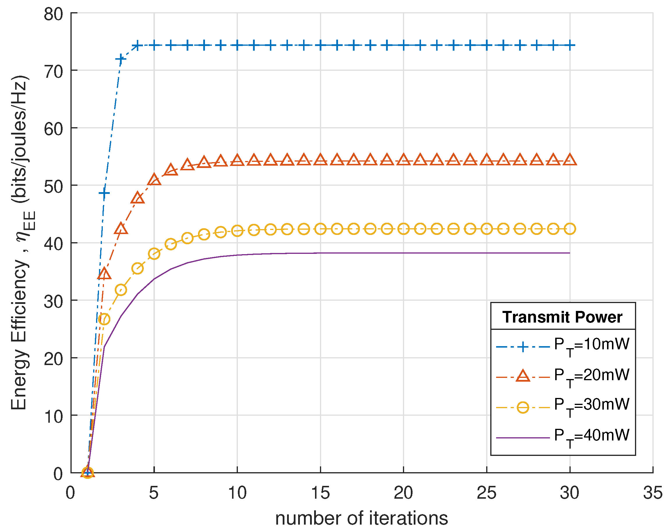
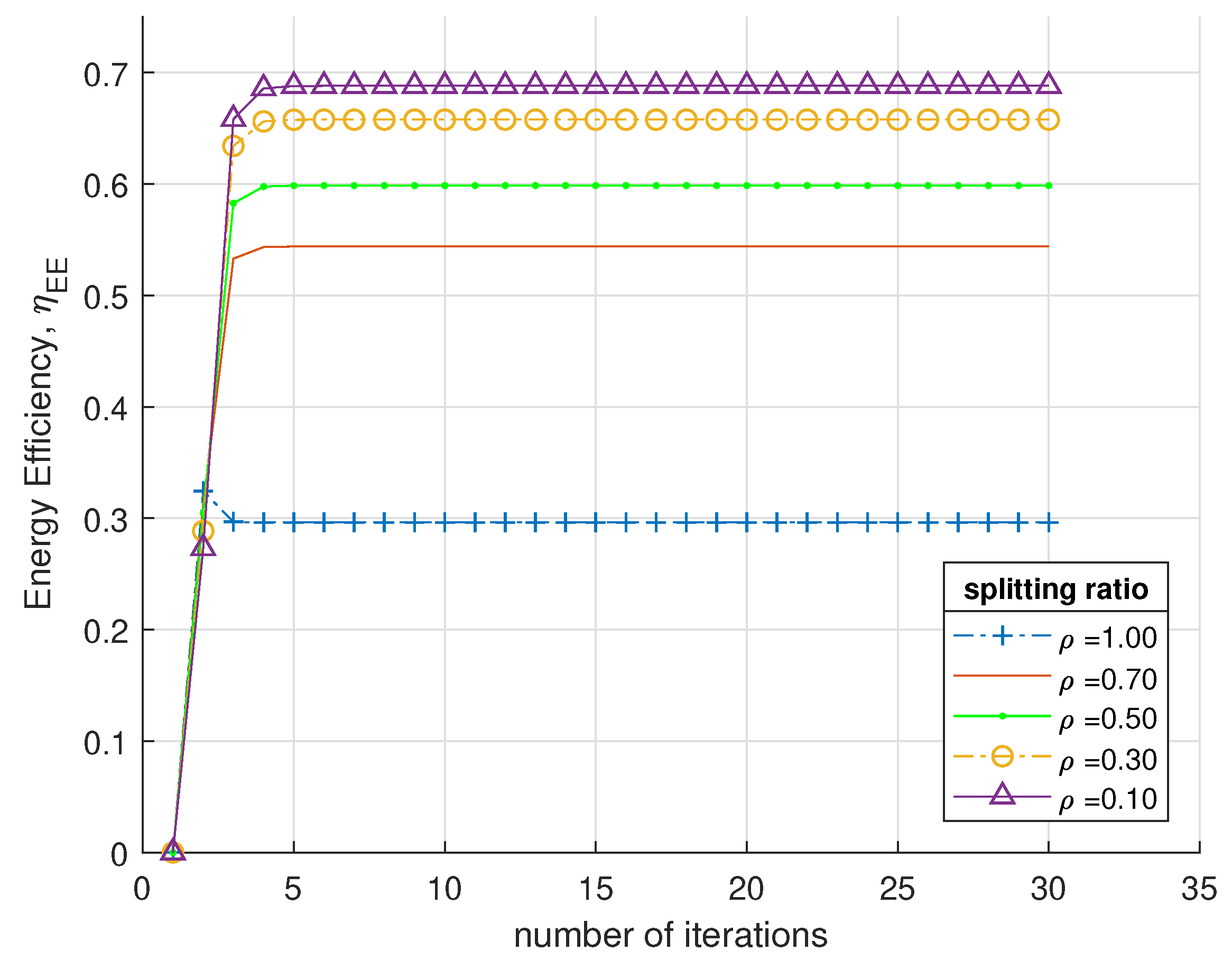
For the proposed Algorithm 2, numerical results are shown in Figure 6 and Figure 7. The Figure 6 plots EE vs. the number of iterations with acceptable tolerance. The EE of the proposed algorithm completely converges after first ten iterations. When transmit power is minimum, maximum energy is supplied to the EH part of the receiver in PS mode. The peak EE is achieved with transmit power 40 mW in the PS mode. In Figure 7, the relationship between the number of iterations and EE is shown using PS ratios over interval $[0,1]$. The EE decreases as $\rho$ changes to $0.1,0.3,0.5,0.7$, or 1, and the behavior of EE shown for different PS ratios. It is noteworthy to compare the convergence time for different scenarios in Figure 6 and Figure 7 with specified iterations in PS mode. In addition, the PS ratio decrease as EE increase and convergence obtained after the initial five iterations.

4.2. Effective Throughput and Outage Target Rate in Power Splitting Mode

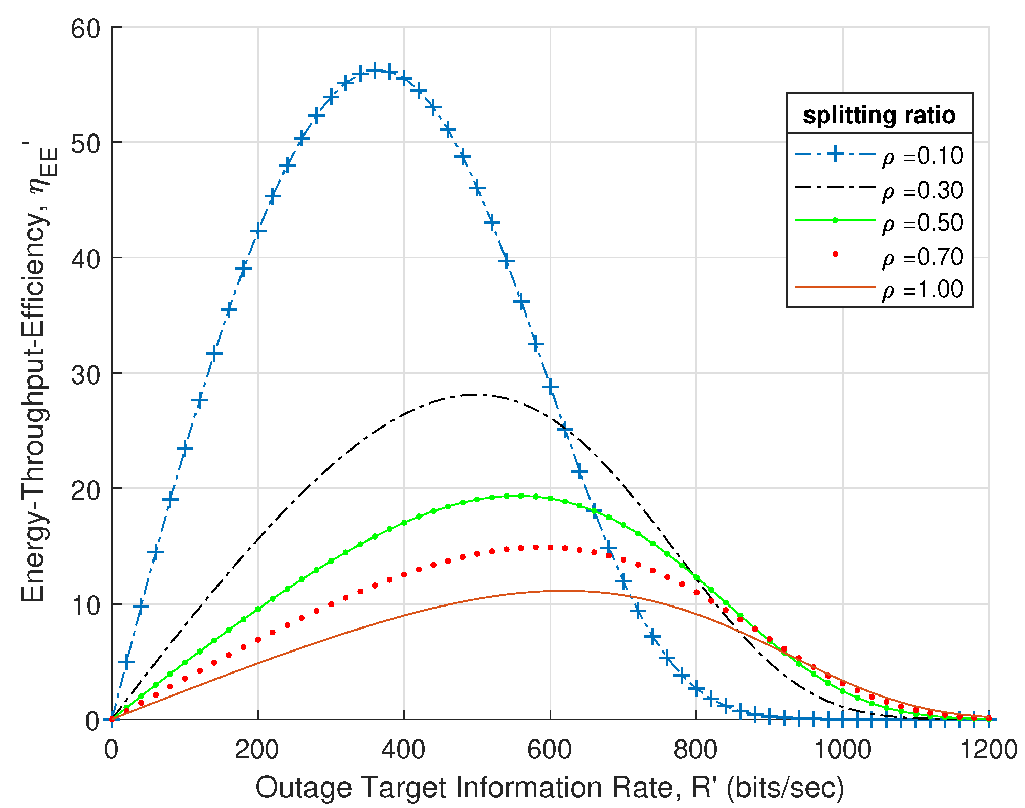
In Figure 8, a relationship of outage targeted rate and energy-throughput efficiency is investigated. Figure 8 illustrates energy-throughput efficiency with different PS ratios. The ${\eta }_{EE}^{\prime }$ is quasi-concave energy function with respect to outage targeted information rate. When the splitting ratio is minimum, the maximum energy is supplied to the EH part of the receiver which achieves peak energy-throughput efficiency. Furthermore, when $\rho$ set to 1, almost negligible EH at the receiver. The energy-throughput efficiency is maximized for different PS ratios.

4.3. Algorithm Convergence and Energy Efficiency in Time Switching Mode

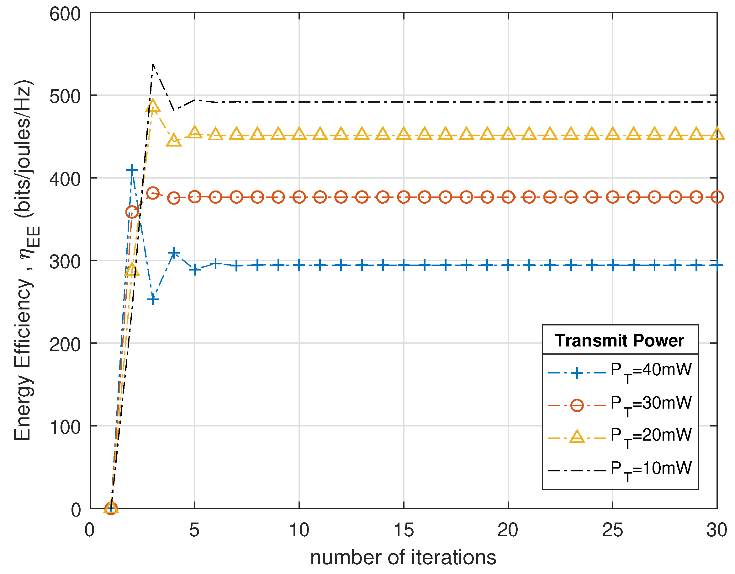
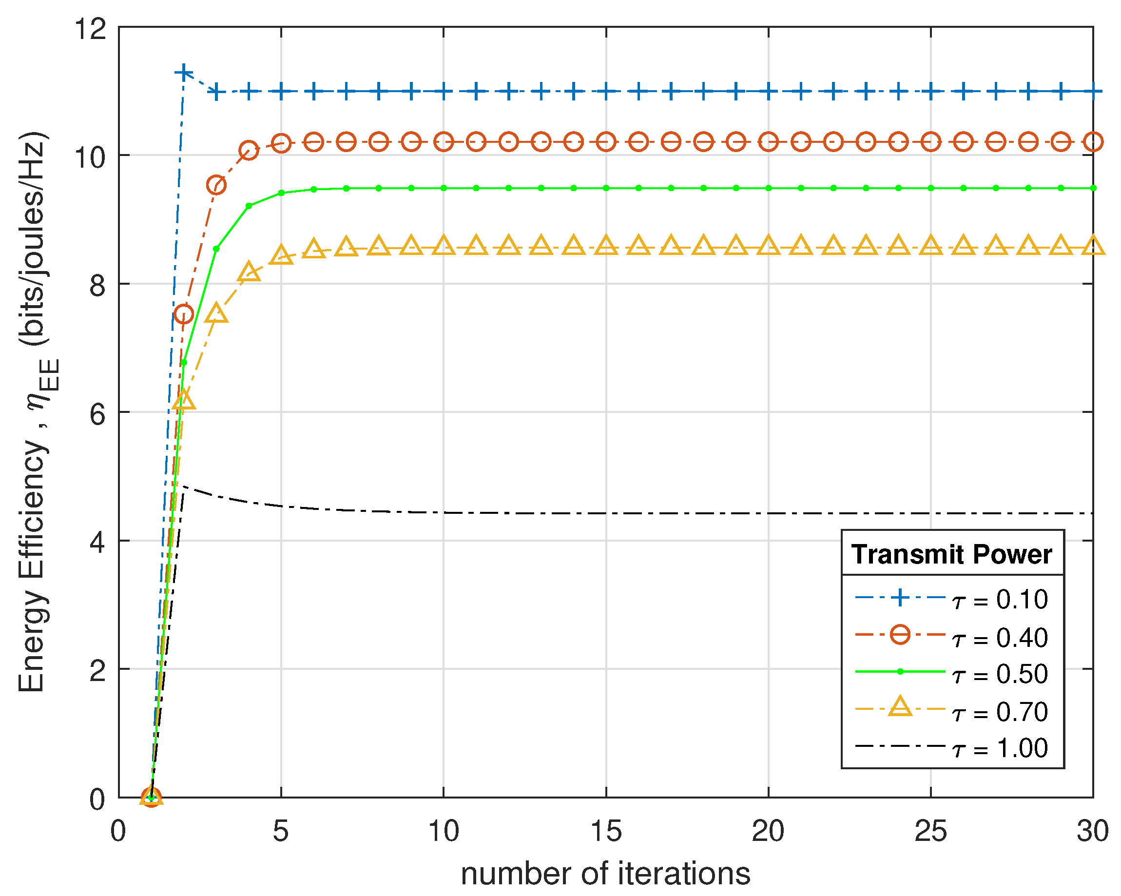
Figure 9 and Figure 10 show the numerical results of the proposed Algorithm 3 in the TS mode. In Figure 9, the convergence of the proposed algorithm is obtained after five iterations. When transmit power is minimum, maximum energy is supplied to the EH part of the receiver in TS mode. In Figure 10, EE decreases as $\tau$ changes to $0.1,0.4,0.5,0.7,$ or 1, and the behavior of EE is shown for different TS ratios. The TS ratio decrease as EE increase, and convergence is achieved after five iterations.

4.4. Effective Throughput and Outage Target Rate in Time Switching Mode

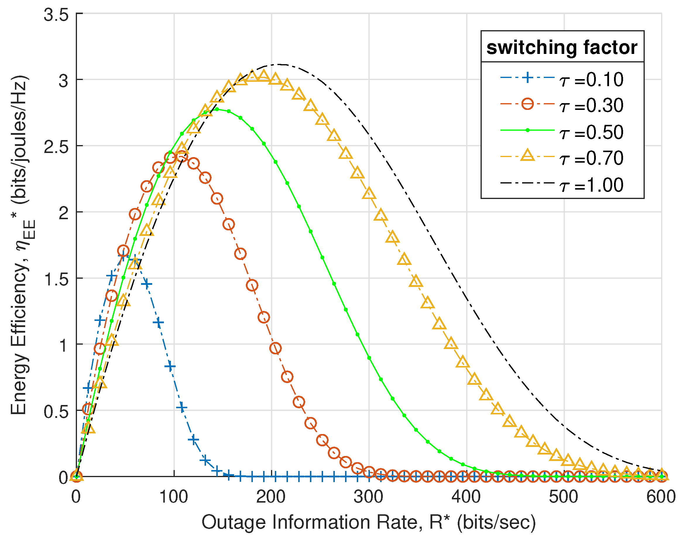
The Figure 11 illustrates energy-throughput efficiency with different TS ratios. The ${\eta }_{EE}^{\prime }$ is quasi-concave energy function with respect to outage targeted information rate. When TS ratio is minimum, the maximum energy is supplied to the EH part of the receiver which achieves peak energy-throughput efficiency. Furthermore, when $\tau$ set to 1, it is almost negligible EH at the receiver. The energy-throughput efficiency maximized with different TS ratios.

5. Conclusions

This paper studied the EE maximization problem and proposed algorithms to solve the optimization problem in PS and TS mode. Simulation results elucidated that EE is essential in SWIPT transceiver design and EE can be improved by modifying parameters in the practical considerations. The proposed algorithm converged towards the optimal solution by PS and TS ratios in fewer iterations. It is worth noting that EE improved by regulating PS and TS ratios using a power splitter and from varying-time-slots, respectively. For the EE improvement, EH is one of the most promising solutions. Analysis of this work will assist understanding SWIPT framework and EE improvements in WSNs. Our future research can stretch out to the EE maximization at the design level.

References

- Krikidis, I.; Timotheou, S.; Nikolaou, S.; Zheng, G.; Ng, D.W.K.; Schober, R. Simultaneous wireless information and power transfer in modern communication systems. IEEE Commun. Mag. 2014, 52, 104–110. [Google Scholar] [CrossRef] [Green Version]
- Perera, T.D.P.; Jayakody, D.N.K.; Sharma, S.K.; Chatzinotas, S.; Li, J. Simultaneous wireless information and power transfer (SWIPT): Recent advances and future challenges. IEEE Commun. Surv. Tutor. 2017, 20, 264–302. [Google Scholar] [CrossRef]
- Belo, D.; Georgiadis, A.; Carvalho, N.B. Increasing wireless powered systems efficiency by combining WPT and electromagnetic energy harvesting. In Proceedings of the IEEE Wireless Power Transfer Conference (WPTC), Aveiro, Portugal, 5–6 May 2016; Volume 17, pp. 1–3. [Google Scholar]
- Zhan, C.; Zhao, H.; Li, W.; Zheng, K.; Yang, J. Energy efficiency optimization of simultaneous wireless information and power transfer system with power splitting receiver. In Proceedings of the IEEE 25th Annual International Symposium on Personal, Indoor, and Mobile Radio Communication, Washington, DC, USA, 2–5 September 2014; pp. 2135–2139. [Google Scholar]
- Clerckx, B.; Zhang, R.; Schober, R.; Ng, D.W.K.; Kim, D.I.; Poor, H.V. Fundamentals of wireless information and power transfer: from RF energy harvester models to signal and system designs. arXiv, 2018; arXiv:1803.07123. [Google Scholar]
- Yu, H.; Zhang, Y.; Guo, S.; Yang, Y.; Ji, L. Energy efficiency maximization for WSNs with simultaneous wireless information and power transfer. Sensors 2017, 17, 1906. [Google Scholar] [CrossRef] [PubMed]
- Pan, G.; Lei, H.; Yuan, Y.; Ding, Z. Performance analysis and optimization for SWIPT wireless sensor networks. IEEE Trans. Commun. 2017, 65, 2291–2302. [Google Scholar] [CrossRef]
- Xiong, K.; Wang, B.; Liu, K.J.R. Rate-energy region of SWIPT for MIMO broadcasting under nonlinear energy harvesting mode. IEEE Trans. Wirel. Commun. 2017, 16, 5147–5161. [Google Scholar] [CrossRef]
- Liu, M.; Liu, Y. Power Allocation for secure SWIPT systems with wireless-powered cooperative jamming. IEEE Commun. Lett. 2017, 21, 1353–1356. [Google Scholar] [CrossRef]
- Liu, Y. Wireless information and power transfer for multirelay-assisted cooperative communication. IEEE Commun. Lett. 2016, 20, 784–787. [Google Scholar] [CrossRef]
- Zheng, H.; Xiong, K.; Fan, P.; Zhou, L.; Zhong, Z. SWIPT-Aware Fog Information Processing: Local Computing vs. Fog Offloading. Ad Hoc Netw. 2018, 18, 3291. [Google Scholar] [CrossRef] [PubMed]
- Kim, D.I.; Moon, J.H.; Park, J.J. New SWIPT using PAPR how it works. IEEE Wirel. Commun. Lett. 2016, 5, 672–675. [Google Scholar] [CrossRef]
- Hu, J.; Yang, Q.; Kwak, K.S. Energy efficiency and delay tradeoff in wireless powered communication networks. In Proceedings of the 2017 17th International Symposium on Communnication and Information Technologies (ISCIT), Cairns, QLD, Australia, 25–27 September 2017; pp. 1–5. [Google Scholar]
- Lu, X.; Wang, P.; Niyato, D.; Kim, D.I.; Han, Z. Wireless charging technologies: Fundamentals, standards, and network applications. IEEE Commun. Surv. Tutor. 2015, 18, 1413–1452. [Google Scholar] [CrossRef]
- Yang, G.; Ho, C.K.; Guan, Y.L. Multi-antenna wireless energy transfer for backscatter communication systems. IEEE J. Sel. Areas Commun. 2015, 33, 26–32. [Google Scholar] [CrossRef]
- Wu, Q.; Tao, M.; Ng, D.W.K.; Chen, W.; Schober, R. Energy-efficient resource allocation for wireless powered communication networks. IEEE Trans. Wirel. Commun. 2016, 15, 2312–2327. [Google Scholar] [CrossRef]
- Vamvakas, P.; Tsiropoulou, E.E.; Vomvas, M.; Papavassiliou, S. Adaptive power management in wireless powered communication networks: A user- centric approach. In Proceedings of the 2017 IEEE 38th Sarnoff Symposium, Newark, NJ, USA, 18–20 September 2017; pp. 1–6. [Google Scholar]
- Tsiropoulou, E.E.; Mitsis, G.; Papavassiliou, S. Interest-aware energy collection and resource management in machine to machine communications. Ad Hoc Netw. 2018, 68, 48–57. [Google Scholar] [CrossRef]
- Tuan, P.V.; Koo, I. Robust weighted sum harvested energy maximization for SWIPT cognitive radio networks based on particle swarm optimization. Sensors 2017, 17, 2275. [Google Scholar] [CrossRef] [PubMed]
- Huang, Y.; Liu, M.; Liu, Y. Energy-efficient SWIPT in IoT distributed antenna systems. IEEE Internet Things J. 2018, 5, 2646–2656. [Google Scholar] [CrossRef]
- Boyer, C.; Roy, S. Invited paper—Backscatter communication and RFID: coding, energy, and MIMO analysis. IEEE Trans. Commun. 2014, 62, 770–785. [Google Scholar] [CrossRef]
- Zhu, F.; Gao, F.; Yao, M. A new cognitive radio strategy for SWIPT system. In Proceedings of the 2014 International Workshop on High Mobility Wireless Communications, Beijing, China, 1–3 November 2014; pp. 73–77. [Google Scholar]
- Zhou, X. Training-based SWIPT: Optimal power splitting at the receiver. IEEE Trans. Veh. Technol. 2015, 64, 4377–4382. [Google Scholar] [CrossRef]
- Jameel, F.; Faisal; Haider, M.A.A.; Butt, A.A. A technical review of simultaneous wireless information and power transfer (SWIPT). In Proceedings of the 2017 International Symposium on Recent Advances in Electrical Engineering (RAEE), Islamabad, Pakistan, 24–26 October 2017; pp. 1–6. [Google Scholar]
- Chu, Z.; Johnston, M.; Goff, L.S. SWIPT for wireless cooperative networks. Electron. Lett. 2015, 51, 536–538. [Google Scholar] [CrossRef]
- Liu, J.; Xiong, K.; Fan, P.; Zhong, Z. RF energy harvesting wireless powered sensor networks for smart cities. IEEE Access 2017, 5, 9348–9358. [Google Scholar] [CrossRef]
- Lee, H.; Song, C.; Choi, S.; Lee, I. Outage probability analysis and power splitter designs for SWIPT relaying systems with direct link. IEEE Commun. Lett. 2017, 21, 648–651. [Google Scholar] [CrossRef]
- Yang, W.; Mou, W.; Xu, X.; Yang, W.; Cai, Y. Energy efficiency analysis and enhancement for secure transmission in SWIPT systems exploiting full duplex techniques. IET Commun. 2016, 10, 1712–1720. [Google Scholar] [CrossRef]
- Shah, S.T.; Choi, K.W.; Lee, T.J.; Chung, M.Y. Outage probability and throughput analysis of SWIPT enabled cognitive relay network with ambient backscatter. IEEE Internet Things J. 2018, 5, 3198–3208. [Google Scholar] [CrossRef]
- Baroudi, U. Robot-assisted maintenance of wireless sensor networks using wireless energy transfer. IEEE Sens. J. 2017, 17, 4661–4671. [Google Scholar] [CrossRef]
- Sun, J.; Zhang, W.; Sun, J.; Wang, C.; Chen, Y. Energy-spectral efficiency in simultaneous wireless information and power transfer. In Proceedings of the 2016 IEEE/CIC International Conference on Communications in China (ICCC), Chengdu, China, 27–29 July 2016; pp. 1–6. [Google Scholar]
- Zhang, H.; Wang, B.; Jiang, C.; Long, K.; Nallanathan, A.; Leung, V.C.M. Energy efficient dynamic resource allocation in NOMA networks. In Proceedings of the GLOBECOM 2017—2017 IEEE Global Communications Conference, Singapore, Singapore, 4–8 December 2017; pp. 1–5. [Google Scholar]