Multi-Objective Control of Air Conditioning Improves Cost, Comfort and System Energy Balance


Department of Electrical Engineering, University of Hawaii at Manoa, Honolulu, HI 96822, USA
*
Author to whom correspondence should be addressed.
Energies 2018, 11(9), 2373; https://doi.org/10.3390/en11092373
Submission received: 6 August 2018
/
Revised: 6 September 2018
/
Accepted: 6 September 2018
/
Published: 8 September 2018
(This article belongs to the Special Issue Building Energy Use: Modeling and Analysis)
Abstract
:A new model predictive control (MPC) algorithm is used to select optimal air conditioning setpoints for a commercial office building, considering variable electricity prices, weather and occupancy. This algorithm, Cost-Comfort Particle Swarm Optimization (CCPSO), is the first to combine a realistic, smooth representation of occupants’ willingness to pay for thermal comfort with a bottom-up, nonlinear model of the building and air conditioning system under control. We find that using a quadratic preference function for temperature can yield solutions that are both more comfortable and lower-cost than previous work that used a “brick wall” preference function with no preference for further cooling within an allowed temperature band and infinite aversion to going outside the allowed band. Using historical pricing data for a summer month in Chicago, CCPSO provided a 1% reduction in costs vs. a similar “brick-wall” MPC approach with the same comfort and 6–11% reduction in costs vs. other control strategies in the literature. CCPSO can also be used to operate the building with much greater comfort and costs or much lower costs and comfort than the “brick-wall” approach, depending on user preferences. CCPSO also reduced peak-hours demand by 3% vs. the “brick-wall” strategy and 4–14% vs. other strategies. At the same time, the CCPSO strategy increased off-peak energy consumption by 15% or more vs. other control methods. This may be valuable for power systems integrating large amounts of renewable power, which can otherwise become uneconomic due to saturation of demand during off-peak hours.
Keywords:
heating ventilation and air conditioning (HVAC); model predictive control (MPC); demand response; EnergyPlus; particle swarm optimization (PSO); renewable energy; smart gridsMSC:
49M37; 65K05; 90-04; 90B35; 90B50; 90C29; 90C56; 90C90; 91B08; 91B10; 91B26; 91B42; 91B74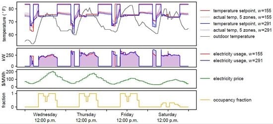
1. Introduction
In recent years, networked computation has become nearly ubiquitous, and power systems have begun relying more heavily on renewable power and market-based settling of supply and demand. These trends create both a need and an opportunity for dynamic pricing and demand response to help balance the power system. In a smart grid environment, price-responsive customers and devices can reschedule electricity loads from the times when electricity supply is scarce and production costs are high to times when supply is abundant and costs are low, thereby reducing bills and also improving the supply-demand balance for the power system as a whole. For example, [1] shows a method for incorporating demand response into day-ahead procurement with renewable energy; [2] reports on savings achievable by industrial customers with dynamic pricing, and [3] discusses savings available to small customers.
Air conditioning systems in buildings provide a rich opportunity for demand response. Buildings account for 40% of all electricity consumed in the United States, with half that figure attributed to heating, ventilation and air conditioning (HVAC) [4].
There is an extensive literature on adjusting the timing of air conditioner operation in commercial buildings to reduce demand during high-cost times and increase it in low-cost times. This uses the building’s thermal mass as a form of thermal storage that has the same effect as an electric battery. It is helpful to divide previous work into three categories: optimal control using detailed building models and simplified user preferences, optimal control with realistic user preferences and simplified building models, or heuristic approaches that choose setpoints based on time-of-day or electricity price alone. This paper introduces a new control strategy that spans the first two classes—optimal control with realistic user preferences and a detailed building model.
The first class of price-responsive control algorithms all seek to shift air conditioner operation between hours while maintaining temperatures within a narrow band that preserves occupant comfort. For example, several authors used simple control algorithms with “brick-wall” temperature limits to investigate the aggregate load-shifting potential of HVAC systems: [5] used such an algorithm to show that electricity demand need not be considered as purely inelastic; [6] used such an algorithm as part of an effort to estimate the effects of large scale adoption of demand response technologies, and [7] used a “brick-wall” algorithm to estimate the potential flexibility of residential HVAC loads in smart grids. Others in the first class of algorithms focus on the savings available to individual customers in a dynamic pricing environment [8], possibly addressing specific technological innovations in the building [9]. Among the customer-focused algorithms, one of the most advanced was introduced by Corbin, Henze, and May-Ostendorp [10]. They use Particle Swarm Optimization (PSO) [11] with a detailed thermal simulation in open-source EnergyPlus building simulation software [12] to perform model predictive control of the HVAC system in a commercial office building. Although Corbin et al. do not mention it, their algorithm represents a sort of “gold standard” for building control—it is able to directly optimize HVAC operation throughout the day to minimize costs under time-varying pricing, using state-of-the-art building simulation software to directly account for the complex, nonlinear behavior of the coupled building and HVAC system.
However, there is one significant shortcoming in the algorithms in this first class—they all use a “brick wall” representation of people’s preferences for comfort, assuming the occupants are indifferent within a narrow range around an ideal temperature, but will not tolerate temperatures outside this range. This assumption produces solutions that generally peg the temperature at the lower edge of the allowed band during pre-cooling times and at the upper edge of the allowed band during other times. This likely does not match true occupant preferences, and foregoes opportunities to make occupants more comfortable when prices are low, and also to move slightly outside the standard comfort band for greater savings when prices are high or occupancy is low.
The second class of algorithms uses more realistic functions to represent customer preferences. These add a term to the cost calculation (objective function) representing users’ willingness to pay to move closer to the ideal temperature. This term takes a few shapes: linear in absolute deviation from the ideal temperature ([13] used this as part of an Immune Clonal Selection algorithm, and [14] used this in a linear program); a “bathtub” shape with a curved bottom and plateaus on either side ([15] is a classic example, and [16] is a more recent instance); or a quadratic curve with a minimum at the ideal temperature ([17] used this with occupancy prediction for a single room, and [18] used it with zonal occupancy predictions for 2–3 zone buildings). Unlike the first class of algorithms, the second class are able to choose settings that increase user comfort when low costs justify it, or relax temperature settings further when customers would prefer that due to high cooling costs. This has the potential to produce solutions that give a better balance of cost vs. comfort, depending on each customer’s preferences. They could also potentially provide more flexiblity to the power system, since they will give deeper demand reductions in times of scarcity and greater increases in times of abundance.
However, all of the algorithms we have identifed in this second class represent the building itself via simplified linear or quadratic models of the building’s response to setpoints. As a consequence, they cannot model the complex, nonlinear behavior of the building. This encompasses a number of factors that strongly affect HVAC energy demand, including variations in efficiency based on equipment loads, outdoor temperatures or humidity; activation of economizers and reheat; “coasting” behavior when cooling setpoints exceed actual air temperatures, and full-load operation when the building cannot immediately reach setpoints. Consequently, although previous algorithms in this class can closely follow user preferences, they do not optimize operation of the building itself as precisely as Corbin et al.’s PSO method [10].
A third class of algorithms uses heuristic methods to select air conditioner setpoints. Night-setback control is a well-established strategy where air conditioning setpoints are raised to a fixed level during unoccupied times and then lowered to a comfortable temperature during occupied times [19]. Another approach is to raise setpoints when prices are high and lower them when prices are low, using price-temperature relationships provided by the authors. For example, [20] adjusts setpoints based on differences between hourly prices and the daily mean price, and [21] adjusts setpoints based on the price difference from a fixed, low threshold and also the difference between the current temperature and the desired temperature.
In this study, we introduce a new model predictive control algorithm for commercial building air conditioners that we call “cost-comfort particle swarm optimization” (CCPSO). This algorithm combines the best of the first two types of approach: precise optimization via a detailed, nonlinear building model and a direct consideration of user preferences for cost savings vs. comfort.
We compare the performance of CCPSO to representative models from each of the control classes discussed above: a “brick wall” PSO approach [10], standard night-setback [19], the “transactive power” heuristic [20] and a linearized building model with the same quadratic treatment of comfort as CCPSO [18]. We find that CCPSO can produce solutions that are simultaneously superior in both cost and comfort to the other strategies. We also find that CCPSO time-shifts power demand more strongly than the other strategies, potentially improving the system’s ability to help balance time-varying supply and demand. This attribute will be especially important in future, high-renewable power systems.
2. Methods
In this section, we describe the CCPSO model and inputs. The complete input data, code and results used for this study are available in the Supplementary Information.
2.1. Optimization Problem
CCPSO selects temperature setpoints for a building HVAC system with the goal of maximizing net benefit to the building occupants—the value of comfort minus electricity costs. Setpoints are selected and evaluated for a sequence of future timesteps, so that the algorithm can pre-cool the building when electricity prices are low or “coast” without cooling when prices are high. At any timestep, the building fabric may be warmer or colder than the long-run average. This thermal energy—or lack of it—constitutes work deferred or stored by the HVAC system, which could result in higher or lower costs in later timesteps. It is not possible to directly assign a financial value to the energy stored in the building fabric, because it depends on electricity prices, occupancy and weather in later timesteps, as well as the strategy used to respond to those conditions. So CCPSO uses two methods to assess this value indirectly.
First, although we expect CCPSO to be run once per day or more often, the planning period extends more than 24 h into the future. This forces the model to consider—and optimize—how energy in the building mass at the end of the first day will affect costs on later days.
Second, the planning period is followed by a standardized “termination period”, with pre-specified setpoints, to assign a financial value to thermal energy in the building fabric at the end of the planning period. Without these extra days, the algorithm could be biased toward leaving the building underconditioned at the end of the planning period, since that would reduce costs during the planning period with no apparent negative impact on later days. The termination period also returns the building model to a standard state before evaluating other setpoints. As will be discussed below, for our example building, we found that cooling decisions on one day have a minimal effect on the state of the building one week later, so the termination period may not strongly influence decisions about the first day of operation. However, the termination period is also needed as part of the thermal modeling process (discussed further below), and performing cost and comfort assesment during this period may increase accuracy somewhat.
In concrete terms, the problem to be solved each day by CCPSO is given by
To solve this problem, optimal setpoints must be found for the planning period, timeblocks H on days 1 to . The function represents the benefit of the thermal comfort in the corresponding time and location if the system uses setpoints , i.e., the amount the building owner would be willing to pay for this amount of cooling. The function represents the cost of purchasing electricity to run the HVAC system with these setpoints. Below, we discuss the computation of these functions in more detail.
In order to reduce the dimensionality of and achieve faster solutions, the problem in Equation (1) includes two simplifications. The time blocks are hourly from midnight to noon, then one block for 12:00 p.m. to 7:00 p.m. and one more for 7:00 p.m. to midnight. This provides high resolution during pre-cooling and high-occupancy periods and a sparser representation during coasting and low-occupancy periods. In addition, rather than choosing different temperature setpoints for each zone, we choose a single setpoint for each time block and apply it to all zones. This representation reduces the problem size while still allowing detailed modeling of pre-chilling strategies. This creates a dimensional similar to [10].
2.1.1. Economic Demand for Cooling
We are not aware of any literature describing building managers’ demand for cooling services, so we use a simple, plausible form. First, we make the following assumptions:
Assumption 1.
If cooling were free, managers would cool to the temperature that makes the most occupants thermally neutral, tideal (assumed to be 72.5 °F in this paper);
Assumption 2.
the amount of cooling that would be selected declines as the cost of cooling rises;
Assumption 3.
the relationship expressed in Assumption 2 is linear; and
Assumption 4.
the perceived benefit of cooling is proportional to building occupancy, measured in person·hours.
Assumption 1 reflects rational behavior; Assumption 2 expresses the economic “law of demand”; Assumptions 3 and 4 are hypothesized for the purpose of this paper. Below, we test a range of proportionality constants for Assumption 3; future work could use field research to estimate both the form and coefficients for the demand function to improve on Assumptions 3 and 4.
With these assumptions, we obtain a demand function for cooling during a given timestep:
where p is the marginal cost of cooling the building ($/°F), 2 is introduced to help with integration later, w is a linear proportionality constant (in $/(°F2·person·hour)), c is the amount of cooling applied (°F), is the amount of cooling needed to reach , o is the building occupancy (number of people) and is the duration of the timestep (hours). The standard interpretation of this demand function is that p is the amount that the manager would be willing to pay for one more unit of cooling, when already obtaining c units of cooling. Thus, the total value that the manager places on c units of cooling can be calculated by integrating the demand function:
Here, we have used , where is the building temperature with no cooling and is the actual temperature. For optimization purposes, we may ignore , the benefit of cooling to , which is constant. This leaves a discomfort index that can be included in the optimization:
With this discomfort index and a change of sign, Equation (1) becomes
Note that Equation (5) can be interpreted as a multi-objective optimization problem minimizing discomfort and cost, where w is a weight or penalty charge used to reconcile the two objectives. By varying the value of w, it is possible to choose an operating strategy anywhere on the Pareto frontier for these two objectives—trading off between minimum cost and minimum discomfort. The algorithm described here allows users to choose any point along this frontier.
2.1.2. Electricity Cost
If forecasts of future electricity prices, building occupancy and weather conditions are available, then the cost of electricity can be calculated as , where is the electricity price during timestep s of day d, and is the amount of electricity used by the HVAC system during that timestep, in response to the setpoints . This gives the objective function:
Section 2.2 shows how we choose values of to solve this optimization problem, Section 2.3 discusses how we compute and from and Section 2.4 discusses the specific data we used for this work. Section 3 presents our results.
2.2. Particle Swarm Optimization
For real-world HVAC systems, the problem given by Equation (6) is inherently non-convex. For example, turning off the cooling system and “coasting” during one time block (by assigning a high value to for that period) may be a locally optimal strategy, but not globally optimal. Furthermore, the most natural method for calculating cost and comfort due to the choice of —building simulation, as discussed in Section 2.3—does not yield derivatives for the objective function. Consequently, this problem must be solved via a derivative-free, global optimization method. For this work, we use particle swarm optimization (PSO) to do this.
As originally described by Kennedy, Eberhart and Shi [11], PSO is a meta-heuristic that progressively refines a population (swarm) of candidate solutions (particles) per iteration (generation); it is suited well for global optimization problems. Inspired by flocking movements of fish and birds, it makes few assumptions about the search space and does not require the problem to be differentiable. We use a PSO variant [22] that utilizes a logarithmically-decreasing inertial weight [23] inspired by findings in [24], alongside the usual cognitive and social attraction weights, and :
Elements of this equation are described in the Nomenclature table, along with the specific values used for this work. The vector-valued quantities, , , and have one component for each time block on each day of the planning period.
Positions of all particles are updated once per generation k, calculated by adding fractions of individual previous velocities, and cognitive and social components. The cognitive component denotes a particle’s memory of its personal best, , against its current position . Similarly, the social component denotes communication of the entire swarm, with comparisons against the swarm’s current best position, . Particles are evaluated by calculating the objective function of Equation (6) with , using EnergyPlus software (8.3.0, U.S. Dept. of Energy, Washington, DC, USA) as discussed in Section 2.3. Using inertia , particles maintain some of their previous trajectory, which is noted to improve exploration properties [25]. Upon completion, is set equal to the best solution in the final iteration k:
To accelerate convergence, the search space for is bounded between 60 °F and 90 °F. If a particle hits the bounds of the search space, it is reflected back into the search space, as if the space was mirrored over the boundary.
To form the initial population, 44 particles are dispersed in the search space using a uniform, random distribution. An additional particle is initialized using a heuristic approach given by:
where is the mean value of for time steps that fall in block h on day d.
Within these constraints, the coefficients are fine-tuned for faster convergence based on interactive testing.
Iteration continues until either , computation time reaches two hours, or the objective function improves by less than $15 over the course of 15 successive iterations.
2.3. EnergyPlus Software
To use the PSO algorithm discussed in Section 2.2, it is necessary to repeatedly calculate the functions and , which show the electricity usage and temperature if setpoints are used for the building’s HVAC system. To perform these computations, we use EnergyPlus software. EnergyPlus is a whole-building energy simulation engine that is widely used in academic and industry research to help design energy-efficient buildings. It can provide highly detailed simulations of the operation and effects of an HVAC system, incorporating factors such as building shape, materials and construction, internal and external gains, and the size of HVAC components.
Normally, EnergyPlus is run as a freestanding program. When run, it initializes the building model, simulates a study period using predefined setpoints, saves results, and then terminates. However, initializing the building model requires significant computational overhead, which slows down the PSO process. Thus, we accelerated the computation by setting up a co-simulation between our Matlab (R2017a, The MathWorks, Inc., Natick, MA, USA) PSO implementation and EnergyPlus, using the MLE+ Matlab toolbox [27]. As shown in Figure 1, EnergyPlus first initializes itself, and then goes into a repeated loop over the planning and termination periods. At each timestep during these periods, EnergyPlus requests setpoints from the Matlab PSO software. By supplying appropriate values, the CCPSO algorithm uses EnergyPlus to efficiently calculate building performance ( and ) over these periods without reinitializing EnergyPlus for each iteration. In our configuration, the termination period uses the same weather and setpoints as were actually used during the time immediately before the planning period. Consequently, after testing candidate settings for the planning period, this technique effectively returns the building model to the same conditions at the start of each iteration, with no wasted calculations.
The CCPSO optimization was run with 20 parallel EnergyPlus workers on a 20-core Linux computer, which were used as needed to simulate the planning and termination periods for each PSO particle during each iteration. Complete code for this model is provided in the Supplementary Information.
2.4. Simulation Parameters
2.4.1. Building Model
We tested the CCPSO algorithm using the benchmark large Chicago office building included with the EnergyPlus installation. This building has exterior walls constructed with eight inches of concrete for the walls and interior floors, possessing a window-to-wall ratio of 38%. The orientation of the building is south, with an aspect ratio of 1.5. The glazing U-value is 3.24 W/m2/K; the solar heat gain coefficient is 0.39. These properties indicate a building with high thermal mass, and follow ASHRAE 90.1-2004.
For all intermediate stories, a single five-zone floor is modeled (north, south, east, west and core), with a multiplier factor of 10. In total, there are 15 zones and 46,320 m2 of conditioned space. The peak occupancy is 2299 people. Each floor is conditioned using a variable air volume (VAV) system with two large water-cooled chillers. A night cycle manager operates in 30 min cycles and an economizer uses outdoor air to provide free cooling when appropriate.
Primary heating and reheating coils are disabled, so that the air conditioning system can be set to “coast” by selecting a high ; in this case, floats until it reaches or establishes thermal equilibrium. A fractional schedule indicates occupancy relative to max, throughout the building. This ranges from zero at night to one during weekday mornings and afternoons, with intermediate values during lunch hours and on weekends. Lighting and equipment are assumed to follow the same fractional schedule as occupancy.
2.4.2. Length of Planning and Termination Periods
As discussed in Section 2.3, each iteration of CCPSO concludes by modeling building performance during a multi-day termination period. This period is used both to evaluate lingering effects of the setpoints chosen during the plannning period, and also to return the simulated building to a state that matches the current state of the real building. For both of these purposes, the termination period must be long enough to return the building to a standard state, which is not affected by any setpoints that were used before the termination period.
In order to choose the termination period length , we conducted a test of the effect of thermal mass on deep cooling operation. For this test, we define a night-setback strategy as follows:
with
Note that reheat is disabled in this building, so the high nighttime setpoints cause the building to “coast” without applying heating or cooling.
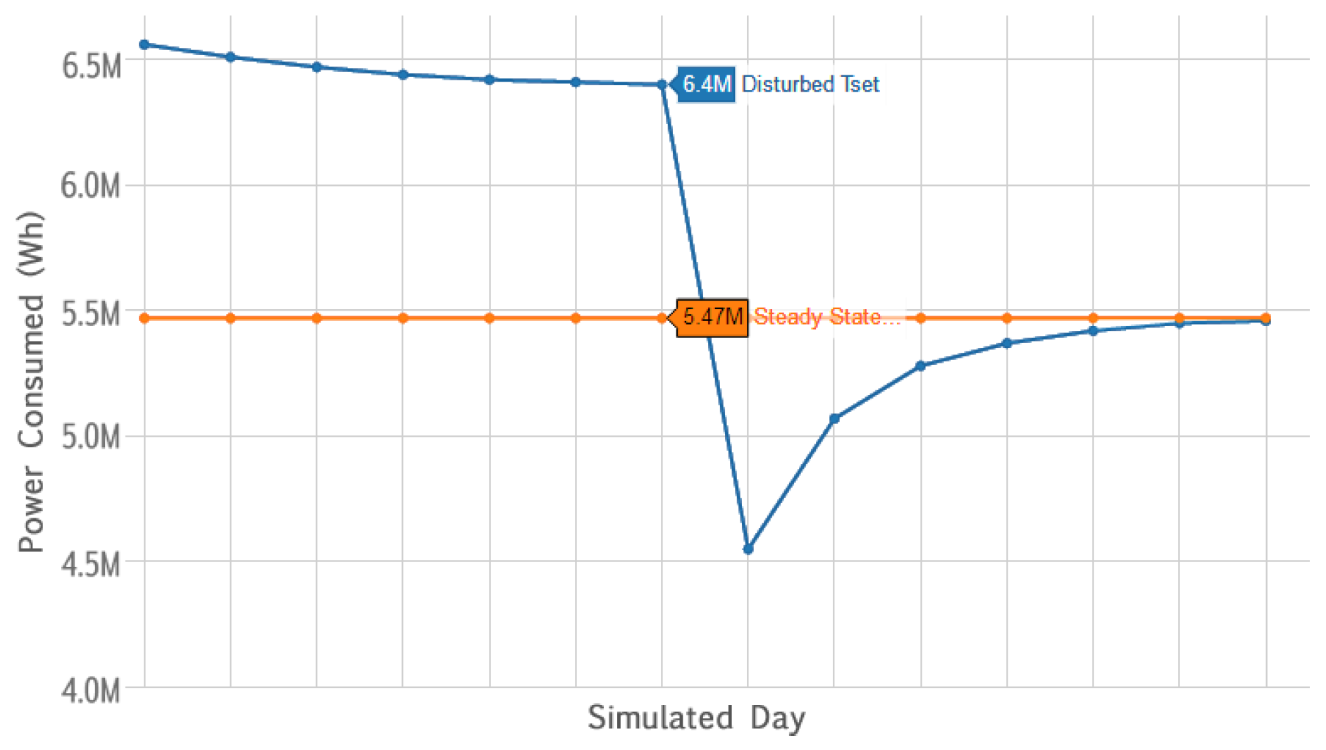
The test is shown in Figure 2 (also see [10]). After reaching steady state using the setpoints given by Equations (11) and (12), an extreme chilling schedule (60 °F) is used continuously until the end of Day 7. Power consumption decreases for several days after the building returns to normal operation; i.e., a normal level of comfort is maintained with less power input. By Day 14, the power consumption and zone temperatures return to within 1% of the steady state values. In this sense, the building “forgets” the extreme perturbation one week earlier. We conclude that the building’s thermal state will be determined almost entirely by the weather and setpoints from the most recent seven days, so we set . We also set the planning period to seven days, in order to ensure that this period includes all the days that could be affected by the binding decisions made for day 1.
2.4.3. Discomfort Penalty
As discussed in Section 2.1, the w parameter can be set by the user to a suitable value to indicate their particular preference for low cost vs. high comfort. Each value of this parameter will drive the algorithm toward a different point on the Pareto frontier of cost vs. comfort. By testing several different values, it is possible to plot part of this frontier. For this work, we chose values of w that produced comfort that spanned a range from about half the discomfort level of the brick-wall PSO strategy, up to slightly less comfortable than the brick-wall strategy. Specifically, we used values for w from the following list:
2.4.4. Electricity Prices
Our reference building is located in the Commonwealth Edison (ComEd) service territory in Chicago, IL, USA. Small ComEd customers can subscribe to flat tariffs where the price-per-kWh component changes only twice a year, e.g., $61 per MWh for summer 2018 [28]. However, large customers are required to sign up for ComEd’s hourly pricing service, which uses a per-kWh charge that is linked directly to the Pennsylvania–Jersey–Maryland (PJM) hourly price. Those charges varied between −$13 and +$106 per MWh in July 2018 [29] (negative prices occurred when wind production was high and demand was low, and wind farms or other generators paid the pool to take their power rather than curtailing it).
2.5. Evaluation Process
We simulated use of the CCPSO algorithm on a rolling basis over the period of 1–31 August 2007. At the start of each simulated day, we retrieved power prices and weather for a 7-day planning period beginning on that day. We used historical weather data for Chicago from the U.S. National Oceanic and Atmospheric Administration [30] and locational marginal power prices from the PJM Interconnection for corresponding days in 2007 (Section 2.4.4). We also retrieved historical conditions for use in the conditioning and termination periods. For the historical period prior to 1 August 2007, we assume the building was operated with the night-setback policy given by Equations (11) and (12). For this test, we assumed perfect foresight of weather and prices.
We then used the PSO algorithm discussed in Section 2.2 to choose optimal setpoints for the coming planning period. Finally, we recorded the weather, setpoints, costs and discomfort from the first day of the planning period for later reference. The recorded values from the first day of each optimization represent the “actual” operation of the simulated system—they are used as the historical conditions for the termination/conditioning period, and are reviewed later to evaluate the performance of the system over the whole study period.
2.6. Benchmarks
To establish benchmarks for evaluation of the CCPSO algorithm, we also ran four previously described control strategies for the same reference office building, prices and weather, as discussed at the end of Section 1. Code to implement each of these algorithms, as described below, is included in the Supplementary Information.
2.6.1. Brick-Wall Particle Swarm Optimization (PSO)
The algorithm reported by Corbin et al. [10] is similar to CCPSO, but with “brick-wall” constraints on temperature. This algorithm requires that setpoints fall strictly within the range 71.6 °F ≤ ≤ 75 °F during occupied hours, but doesn’t assign any other cost to discomfort. The brick-wall PSO is otherwise identical to CCPSO, aside from the performance enhancements noted in Section 2.3. To create benchmarks for CCPSO, we used the brick-wall PSO algorithm to choose setpoints for 1–31 August, then evaluated the total cost and discomfort that would occur over this period, using the discomfort Equation (4).
2.6.2. Night-Setback
Night-setback is a well-established HVAC control strategy, where setpoints are raised to a high level during unoccupied times, allowing the air conditioning system to shutdown or make better use of free cooling [19]. Temperatures are then lowered to a comfortable temperature during occupied times. We evaluated electricity cost and comfort when using the night-setback strategy given by Equation (11), with values for ranging from 72.5° (comfort-seeking) to 75 °F (cost-reducing). Setpoints were 80 °F during unoccupied times.
2.6.3. Transactive Power
The “transactive power” strategy [20] chooses setpoints each hour according to the equation
where r is the electricity price during the current hour, is the mean electricity price for the day, is the standard deviation of electricity prices during the day, is an adjustment factor applied when and is applied when . For our benchmark, we used 80 °F setpoints during unoccupied times and followed the transactive power strategy during occupied times. For precooling configurations, where was nonzero, we also applied the transactive power strategy during the last two hours before occupancy began in the morning. We calculated and based only on the hours when the transactive power strategy was in effect. We tested this strategy with all permutations of , and , as described in [20].
2.6.4. Linearized Building Optimization
Leow et al. [18] report a building control strategy with the same objective function as CCPSO, including a quadratic discomfort term. However, instead of using PSO to optimize setpoints for a detailed building model, they use dynamic programming to directly optimize setpoints for a linearized building model. Their model solves for multiple zones, but when setpoints are the same in all zones, it reduces to a fairly simple form:
where i indexes over the n hours of the study, is the price of electricity during hour i, is the amount of electricity used by the HVAC system during hour i, w is a penalty term identical to CCPSO, is the average air temperature in occupied spaces during hour i and is the preferred temperature. The second line of this problem is a linearized thermal model of the building, where is the effective outdoor temperature during hour i and , and are constant coefficients that are found by regression using historical observations of the building’s behavior. Leow et al. define the effective outdoor temperature each hour as
where is the outdoor air temperature, a is the absorptivity of the building exterior (assumed by Leow et al., to be 0.4), I is the solar irradiance on the building, is an external surface coefficient, assumed to be 20 W/m2 °C, and is the temperature drop due to longwave radiation, assumed to be –6 °C.
To implement the linearized building optimization, we first simulated operation of the reference building for the month of August 2007 using the night-setback strategy with nighttime setpoint of 80 °F and daytime setpoint of 72.5 °F. We then calculated the regression coefficients , and based on the hourly irradiance, energy consumption and temperature data from this simulation. We next used CPLEX software (12.8.0, IBM Corp., Armonk, NY, USA) to solve the model in Equation (15) directly as a quadratic program, producing optimal temperatures for each hour of August 2007. Finally, we used EnergyPlus to simulate operation of the building with setpoints matching these temperature targets, and tabulated the resulting electricity cost and discomfort measures over the month. We repeated this process with values of the w ranging from 200 to 10,000 $/(106 °F2·person·hour).
3. Results and Discussion
In this section, we first illustrate the CCPSO algorithm by showing its behavior for some sample days during the summer cooling period in 2007. We then compare the cost, comfort and load-shifting with CCPSO to four other HVAC control algorithms that represent the major classes of control strategy that we identified in the literature—“brick-wall” PSO [10], standard night-setback, the “transactive power” heuristic [20], and direct optimization using a linearized building model [18]. The setup for each of these is described in Section 2.6.
3.1. Overview of Cost-Comfort Particle Swarm Optimization (CCPSO) Behavior
As discussed in Section 2, CCPSO uses a penalty factor w to indicate preferences for cooling vs. cost-reductions. CCPSO multiplies this penalty factor (in $/(106 °F2·person·hour)), by the discomfort index each hour (in 106 °F2·person·hour), and adds the resulting penalty to the objective function that it minimizes when choosing setpoints for each day. As shown in Equation (4), the discomfort index is calculated based on the building occupancy during each timestep and the difference between the actual temperature in each building zone () and the ideal temperature for occupant comfort (). Consequently, higher values of w drive the algorithm toward more comfortable solutions (closer to ), and lower values drive it toward less expensive solutions.
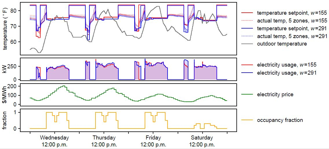
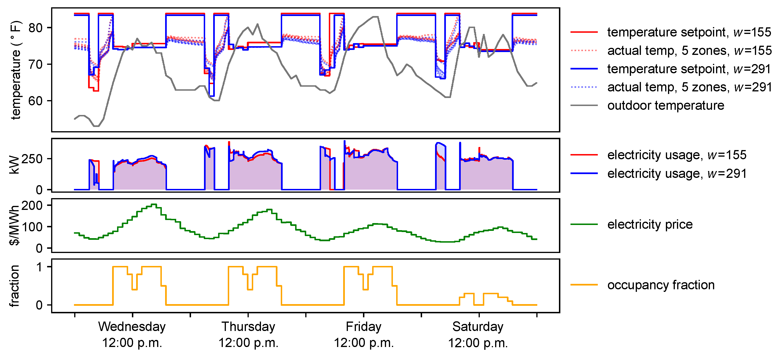
Figure 4 shows four days of behavior for the Chicago office building model in which we tested CCPSO, for two different penalty factors w. CCPSO consistently takes advantage of low electricity prices to pre-chill the building early in the morning. Then, temperatures are allowed to coast by setting high until occupants arrive at 8:00 a.m. As discussed in Section 2.4.1, reheat is disabled in this building, so high setpoints cause the cooling system to shut down but not to heat air. However, as shown by the dotted lines, air temperatures do rise rapidly in some zones during the pre-occupancy coasting period, due to solar heating. The same behavior would occur at this time with standard night-setback. During occupied hours, the controller maintains temperatures close to . When CCPSO is used with a low penalty factor (), it chooses higher temperatures in the afternoon compared to CCPSO with a higher penalty factor (). This allows energy consumption to be reduced during the afternoon or during the pre-cooling period, or both. This effect is stronger on days with high power prices (Wednesday and Thursday).
3.2. Comparison of Cost and Comfort between Control Strategies
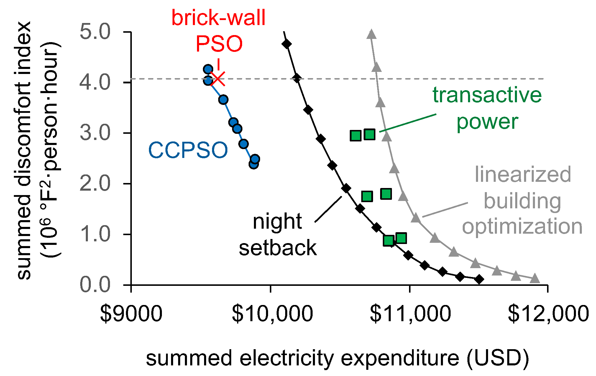
Figure 5 compares cost and comfort levels between CCPSO and four other control strategies from the literature (see Section 2.6). The x-axis shows the total cost of purchasing electricity during the month of August 2007, and the y-axis shows the sum of the discomfort index (Equation (4)) for all timesteps of the month. For each control strategy and parameter value, the cost and discomfort index were calculated by simulating operation of the reference building for the month of August 2007 with standard occupancy levels, using the setpoints provided by each strategy.
Blue points in Figure 5 show results from CCPSO for w values from 155 (top) to 291 (bottom) $/(106 °F2·person·hour). Building managers can select any location along this Pareto frontier, trading off costs vs. discomfort.
The red X shows results from the “brick-wall” PSO algorithm with the authors’ hard temperature boundaries of 71.6–75.2 °F [10]. The brick-wall PSO falls slightly above the frontier found with the CCPSO algorithm, likely because it does not seek to improve comfort within this range during low-cost times or save money by relaxing the range during high-cost times.
Black diamonds in Figure 5 show a standard night-setback strategy with fixed setpoints of 72.5 (bottom) to 75.5 °F (top) during occupied hours and 80 °F at night, following Equation (11). This serves as a reasonable benchmark for other control strategies, since it is a common and easy-to-implement technique. At the lower end, this strategy produces an outcome with much higher electricity costs but also greater comfort than CCPSO. We would expect CCPSO to converge to this point as the penalty factor w is raised, but we didn’t investigate this due to limited computing time.
Green squares in Figure 5 show results from the “transactive power” strategy described in [20]. The authors provide 12 configurations with varying values for three parameters. The six results shown here are for the most comfort settings, “comfortable economy” (top), “balanced comfort” (middle) and “maximum comfort” (bottom). The scenarios on the right use temperatures below to precool when prices are below average, and the scenarios on the left do not (precooling does not appear to work well for this technique in this building). Another six scenarios (“maximum economy”, “balanced economy” and “economical comfort” with or without precooling) fall above the top of this plot. In the “maximum comfort” mode with no precooling, the transactive power strategy costs slightly less than an equally comfortable night-setback strategy. However, with other settings, transactive power performs worse than simple night-setback. It appears that this strategy is not well suited to the complex building studied here, e.g., frequent changes in setpoints in response to changing prices cause the HVAC system to run at inefficient operating levels, and strong responses during high-cost hours reduce comfort.
Finally, the gray points show results from optimizing operation of a linearized building model, as described by [18] and in Section 2.6.4. This model uses the same objective function as CCPSO, but instead of using particle swarm optimization with a detailed building model, it directly optimizes setpoints based on a simple linear model of the building’s thermal behavior. This strategy is somewhat less responsive to the penalty term than CCPSO, and points in Figure 5 correspond to values of w between 568 (top) and 10,000 (bottom) $/(106 °F2·person·hour). In our reference building, for all values of w, the linearized building optimization strategy cost more than an equally comfortable night-setback strategy. We hypothesize that the linearized building model underperforms because it doesn’t incorporate nonlinear building behavior, as discussed in Section 1. For example, high setpoints will cause the air conditioning to shutdown at night, but the linearized building model is unable to anticipate and take advantage of that. The linearized model is also unable to account for the nonlinear effect of setpoints on chiller efficiency or economizer operation.
Within the comfort range shown (2.4–4.2 × 10⁶ °F2·person·hours over the month of August), CCPSO dominates over the other strategies we tested, in the sense that it provides solutions that are simultaneously more comfortable and lower in cost than the other strategies.
3.3. Comparison of Energy Usage between Control Strategies
We next compare the cost and energy usage of the five control strategies shown in Figure 5, when using parameters that give similar comfort. For this comparison, we selected parameters for each strategy that gave the closest comfort level to the brick-wall PSO strategy, i.e., the points nearest to the dotted line in Figure 5.
The third row of Table 1 compares the electricity expenditure among the control strategies when operating at this comfort level. CCPSO has the lowest cost, about 1% below the brick-wall strategy, 6% below a standard night-setback strategy and 11% below the linear building optimization. The closest matching transactive power strategy had greater comfort than CCPSO; however, referring to Figure 5 we see that CCPSO could provide equivalent comfort at a cost of $9800, 8% below the transactive power strategy.
In addition to improving cost and/or comfort for the customer, CCPSO is intended to provide a price response that helps keep the power system balanced. The remaining rows of Table 1 compare the price response between these HVAC control strategies. The first four strategies use a similar total amount of electricity. Compared to night-setback, the PSO strategies raise total energy use slightly; however, overall costs are reduced by shifting demand to low-cost times. Among the first four strategies, CCPSO shifts consumption most effectively toward low-price times, resulting in the lowest average price per kWh used. Specifically, during hours with the top 5% highest prices, when the power supply is most constrained, CCPSO reduces demand by 3% compared to the brick-wall algorithm, 14% compared to the night-setback strategy and 4% compared to transactive power. During times when power is most abundant, when electricity prices are in the bottom 5%, the CCPSO strategy increases demand by 15% relative to the brick-wall algorithm. The night-setback and transactive power strategies use almost no power during the lowest-priced hours. Increasing consumption during low-cost times may be especially important for enabling power systems to use more renewable power, as one of the key factors limiting adoption of wind and solar power is saturation of demand during sunny, windy and low-load times, which reduces the economic value of renewable power or even causes it to be discarded unused [31,32,33,34,35,36].
The linear building optimization is the most effective of all the strategies at lowering demand during high-price times and raising it during low-price times; however, it also uses more power overall than the other strategies, resulting in a higher total cost for the month.
4. Conclusions
This work introduces a new control algorithm, CCPSO, which seeks to optimize air conditioner temperature setpoints for a commercial building, responding to time-varying electricity prices, in order to minimize cost while maximizing comfort. CCPSO differs from previous work by combining an explicit, continuous model of user preferences for comfort vs. cost savings with a detailed simulation of building thermal behavior. Combining these elements allows CCPSO to optimize closely to building occupants’ preferences, achieving both lower cost and higher comfort than previously reported control strategies. CCPSO also shifts load more strongly from peak to off-peak hours than previously reported strategies, which may be especially important in high-renewable power systems.
Compared to a standard night-setback strategy that achieves similar comfort (75 °C during the day, off during the night), CCPSO reduced power costs by 6% during a month of cooling in Chicago. Compared to previous work using a PSO control algorithm with “brick-wall” constraints (no preference for further cooling within an allowed temperature band, and infinite aversion to going outside the allowed band), CCPSO reduced power costs by about 1%. Although these savings are modest, they come at no additional cost and may be significant for a large building. With the CCPSO algorithm, savings can also be increased or decreased—with a corresponding trade-off in comfort—depending on users’ comfort preferences. CCPSO also outperformed two other methods from the literature—transactive power and optimization via a linearized building model—with financial savings of 8–11% at comparable comfort levels.
Of particular interest for high-renewable power systems, we found that CCPSO is more responsive to dynamic prices than the previous approaches, providing a 3–14% reduction in load during system peaks and ≥15% increase in load during minimum-price times. This response could improve utilization of efficient baseload plants in current-day power systems, and could help integrate renewable power in future power systems, where high and low prices may correspond to scarcity and abundance of renewable power. This shift from peak to off-peak may also provide additional financial savings by reducing demand charges associated with the customer or system’s peak demand. CCPSO offers a “best of both worlds” approach, enabling building managers to find the best balance of cost and comfort, and at the same time improving the supply-demand balance in the rest of the power system, reducing costs for all users.
CCPSO does, however, have some limitations. The main limitation (shared with the brick-wall PSO) is that it is computationally intensive, requiring about 1.25 h to find setpoints for each day on a computer with two 10-core 2.8 GHz Intel Xeon “Ivy Bridge” processors (Intel Corp., Santa Clara, CA, USA). This work only tested CCPSO for a commercial building with fixed day/night occupancy cycles; results may differ significantly for residential HVAC, which has different patterns for each household and different equipment available. As presented here, CCPSO also does not optimize each zone separately, which could allow better trade-offs between comfort and cooling energy, e.g., by providing less cooling in low-occupancy zones. Although this work used a state-of-the-art building simulation model to evaluate performance, CCPSO has not been tested in a physical building environment.
In future work, we plan to address these shortcomings by testing the use of reduced-form models of the building and HVAC to obtain faster solutions, investigating use of CCPSO in a residential context, optimizing individual zones separately, and applying the algorithm in practice in large buildings. We also plan to study opportunities for improved performance via enhanced building thermal memory and incorporate uncertain forecasts peak-demand charges.
Supplementary Materials
The following are available online at https://www.mdpi.com/1996-1073/11/9/2373/s1.
Author Contributions
Conceptualization, M.F. and A.I.; Methodology, M.F. and A.I.; Software, M.F. and A.I.; Validation, A.I.; Formal Analysis, M.F. and A.I.; Investigation, A.I.; Resources, M.F.; Data Curation, M.F. and A.I.; Writing—Original Draft Preparation, A.I.; Writing—Review and Editing, M.F.; Visualization, M.F. and A.I.; Supervision, M.F.; Project Administration, M.F.; Funding Acquisition, M.F.
Funding
This research was funded by U.S. National Science Foundation award number 1310634.
Conflicts of Interest
The authors declare no conflict of interest.
Nomenclature
| Optimization Model | |
| duration of timestep s (hours) | |
| temperature in zone z during time step s on day d, if setpoints are used | |
| most-preferred temperature for building occupants (assumed to be 72.5 °F) | |
| vector of n temperature setpoints for HVAC system for all time blocks on days 1 to (decision variables) | |
| dollar-denominated benefit in zone z during timestep s of day d if the system uses setpoints | |
| cost of purchasing electricity during timestep s of day d if the system uses setpoints | |
| D | sequence of future days used for performance evaluation (1, 2, …, ) |
| amount of electricity used (kWh) during timestep s of day d, if using setpoints | |
| H | sequence of time blocks within each day, for which setpoints are chosen (hours starting at 12:00 a.m., 1:00 a.m., …, 11:00 a.m. and blocks spanning 12:00–7:00 p.m. and 7:00 p.m.–12:00 a.m.) |
| n | number of time steps in planning period () |
| length of planning period (days): number of future days for which optimal setpoints are chosen (7 for this work) | |
| length of termination period (days): additional days used for end-state evaluation (7 for this work) | |
| building occupancy in zone z during time step s on day d (# people) | |
| electricity price during timestep s of day d ($/kWh) | |
| S | sequence of time steps within each day, used for building simulation (12:00–12:05 a.m., 12:05–12:10 a.m., …, 11:55 p.m.–12:00 a.m.) |
| w | amount the building owner is willing to pay to avoid discomfort ($/(°F2·person·hour)) |
| Z | set of building zones (N, S, E, W, Core) |
| Particle Swarm Procedure | |
| temperature setpoints for particle p during iteration k | |
| best-performing particle in full population during iteration k | |
| best-performing version of particle p up through iteration k | |
| , | diagonal matrices of random numbers, uniformly distributed on [0,1], regenerated each iteration |
| velocity of particle p during iteration k | |
| a | acceleration constant (set to 1) |
| inertial weight during iteration k | |
| cognitive attraction weight (0.7) | |
| social attraction weight (1.2) | |
| k | iteration counter |
| maximum allowed number of iterations (200) | |
| P | set of particles in the swarm {1, …, 45} |
| upper and lower bounds on inertia (0.4, 0.9) | |
References
- Kwon, S.; Ntaimo, L.; Gautam, N. Optimal Day-Ahead Power Procurement With Renewable Energy and Demand Response. IEEE Trans. Power Syst. 2017, 32, 3924–3933. [Google Scholar] [CrossRef]
- Nezamoddini, N.; Wang, Y. Real-Time Electricity Pricing for Industrial Customers: Survey and Case Studies in the United States. Appl. Energy 2017, 195, 1023–1037. [Google Scholar] [CrossRef]
- Roldán Fernández, J.M.; Payán, M.B.; Santos, J.M.R.; García, A.L.T. The Voluntary Price for the Small Consumer: Real-Time Pricing in Spain. Energy Policy 2017, 102, 41–51. [Google Scholar] [CrossRef]
- Shaikh, P.H.; Mohd Nor, N.B.; Nallagownden, P.; Elamvazuthi, I.; Ibrahim, T. A review on optimized control systems for building energy and comfort management of smart sustainable buildings. Renew. Sustain. Energy Rev. 2014, 34, 409–429. [Google Scholar] [CrossRef]
- Ilic, M.; Black, J.; Watz, J. Potential Benefits of Implementing Load Control. IEEE Power Eng. Soc. Winter Meet. 2002, 1, 177–182. [Google Scholar] [CrossRef]
- Black, J.W. Integrating Demand into the U.S. Electric Power System: Technical, Economic, and Regulatory Frameworks for Responsive Load. Ph.D. Thesis, Massachusetts Institute of Technology, Cambridge, MA, USA, 2005. [Google Scholar]
- Ali, M.; Safdarian, A.; Lehtonen, M. Demand Response Potential of Residential HVAC Loads Considering Users Preferences. In Proceedings of the IEEE PES Innovative Smart Grid Technologies Europe, Istanbul, Turkey, 12–15 October 2014; pp. 1–6. [Google Scholar] [CrossRef]
- Tiptipakorn, S.; Lee, W.J. A Residential Consumer—Centered Load Control Strategy in Real-Time Electricity Pricing Environment. In Proceedings of the 39th North American Power Symposium, Las Cruces, NM, USA, 30 September–2 October 2007; pp. 505–510. [Google Scholar] [CrossRef]
- Lee, Y.M.; Horesh, R.; Liberti, L. Optimal HVAC Control as Demand Response with On-Site Energy Storage and Generation System. Energy Procedia 2015, 78, 2106–2111. [Google Scholar] [CrossRef]
- Corbin, C.D.; Henze, G.P.; May-Ostendorp, P. A model predictive control optimization environment for real-time commercial building application. J. Build. Perform. Simul. 2013, 6, 159–174. [Google Scholar] [CrossRef]
- Kennedy, J.; Eberhart, R. Particle Swarm Optimization. In Proceedings of the ICNN’95—International Conference on Neural Networks, Perth, Australia, 27 November–1 December 1995; Volume 4, pp. 1942–1948. [Google Scholar] [CrossRef]
- Crawley, D.B.; Lawrie, L.K.; Winkelmann, F.C.; Buhl, W.F.; Huang, Y.J.; Pedersen, C.O.; Strand, R.K.; Liesen, R.J.; Fisher, D.E.; Witte, M.J.; et al. EnergyPlus: Creating a New-Generation Building Energy Simulation Program. Energy Build. 2001, 33, 319–331. [Google Scholar] [CrossRef]
- Hong, Y.Y.; Lin, J.K.; Wu, C.P.; Chuang, C.C. Multi-Objective Air-Conditioning Control Considering Fuzzy Parameters Using Immune Clonal Selection Programming. IEEE Trans. Smart Grid 2012, 3, 1603–1610. [Google Scholar] [CrossRef]
- Nguyen, D.T.; Le, L.B. Joint Optimization of Electric Vehicle and Home Energy Scheduling Considering User Comfort Preference. IEEE Trans. Smart Grid 2014, 5, 188–199. [Google Scholar] [CrossRef]
- Constantopoulos, P.; Schweppe, F.C.; Larson, R.C. ESTIA: A Real-Time Consumer Control Scheme for Space Conditioning Usage under Spot Electricity Pricing. Comput. Oper. Res. 1991, 18, 751–765, (This Preprint Lacks Graphs; They are in 1987 Technical Report and Thesis). [Google Scholar] [CrossRef]
- West, S.R.; Ward, J.K.; Wall, J. Trial Results from a Model Predictive Control and Optimisation System for Commercial Building HVAC. Energy Build. 2014, 72, 271–279. [Google Scholar] [CrossRef]
- Mady, A.E.D.; Provan, G.M.; Ryan, C.; Brown, K.N. Stochastic Model Predictive Controller for the Integration of Building Use and Temperature Regulation. In Proceedings of the 25th AAAI Conference on Artificial Intelligence, San Francisco, CA, USA, 7–11 August 2011. [Google Scholar]
- Leow, W.L.; Larson, R.C.; Kirtley, J.L. Occupancy-Moderated Zonal Space-Conditioning under a Demand-Driven Electricity Price. Energy Build. 2013, 60, 453–463. [Google Scholar] [CrossRef]
- PNNL. Building Re-Tuning Training Guide: Occupancy Scheduling: Night and Weekend Temperature Set Back and Supply Fan Cycling during Unoccupied Hours; Technical Report PNNL-SA-85194; Pacific Northwest National Laboratory: Richland, WA, USA, 2012. [Google Scholar]
- Hammerstrom, D.J.; Ambrosio, R.; Carlon, T.A.; DeSteese, J.G.; Horst, G.R.; Kajfasz, R.; Kiesling, L.L.; Michie, P.; Pratt, R.G.; Yao, M. Pacific Northwest GridWise™ Testbed Demonstration Projects; Part I. Olympic Peninsula Project; Technical Report PNNL-17167; Pacific Northwest National Laboratory (PNNL): Richland, WA, USA, 2007. [Google Scholar]
- Yoon, J.H.; Bladick, R.; Novoselac, A. Demand Response for Residential Buildings Based on Dynamic Price of Electricity. Energy Build. 2014, 80, 531–541. [Google Scholar] [CrossRef]
- Chen, S. Constrained Particle Swarm Optimization, Ver 20130330. 2013. Available online: https://www.mathworks.com/matlabcentral/fileexchange/25986-constrained-particle-swarm-optimization (accessed on 5 August 2018).
- Gao, Y.; An, X.; Liu, J. A Particle Swarm Optimization Algorithm with Logarithm Decreasing Inertia Weight and Chaos Mutation. In Proceedings of the 2008 International Conference on Computational Intelligence and Security, Suzhou, China, 13–17 December 2008; Volume 1, pp. 61–65. [Google Scholar] [CrossRef]
- Bansal, J.; Singh, P.K.; Saraswat, M. Inertia weight strategies in particle swarm optimization. In Proceedings of the 2011 Third World Congress on Nature and Biologically Inspired Computing (NaBIC), Salamanca, Spain, 19–21 October 2011; pp. 633–640. [Google Scholar]
- Shi, Y.; Eberhart, R.C. Empirical study of particle swarm optimization. In Proceedings of the 1999 Congress on Evolutionary Computation, Washington, DC, USA, 6–9 July 1999; Volume 3. [Google Scholar]
- Perez, R.; Behdinan, K. Particle swarm approach for structural design optimization. Comput. Struct. 2007, 85, 1579–1588. [Google Scholar] [CrossRef]
- Bernal, W.; Behl, M.; Nghiem, T.X.; Mangharam, R. MLE+: A Tool for Integrated Design and Deployment of Energy Efficient Building Controls. In Proceedings of the 4th ACM Workshop on Embedded Sensing Systems for Energy-Efficiency in Buildings (BuildSys’12), Toronto, ON, Canada, 6 November 2012. [Google Scholar]
- ComEd. Purchased Electricity Charges: Supplement to Rate BES and Rider PE; Technical Report; Commonwealth Edison Company: Chicago, IL, USA, 2018. [Google Scholar]
- ComEd. Rate BES-H Pricing. 2018. Available online: https://secure.comed.com/MyAccount/MyBillUsage/Pages/RatesPricing.aspx (accessed on 23 August 2018).
- EnergyPlus. EnergyPlus Weather Data by Location. 2015. Available online: https://energyplus.net/weather-location/north_and_central_america_wmo_region_4/USA/IL/USA_IL_Chicago-Midway.AP.725340_TMY3 (accessed on 5 August 2018).
- Matthias Fripp, I.; Roberts, M.J. Variable Pricing and the Cost of Renewable Energy; Technical Report NBER Working Paper No. 24712; National Bureau of Economic Research: Cambridge, MA, USA, 2018. [Google Scholar]
- Fripp, M. Switch: A Planning Tool for Power Systems with Large Shares of Intermittent Renewable Energy. Environ. Sci. Technol. 2012, 46, 6371–6378. [Google Scholar] [CrossRef] [PubMed] [Green Version]
- Bird, L.; Cochran, J.; Wang, X. Wind and Solar Energy Curtailment: Experience and Practices in the United States; Technical Report NREL/TP-6A20-60983; National Renewable Energy Laboratory: Golden, CO, USA, 2014. [Google Scholar]
- Li, C.; Shi, H.; Cao, Y.; Wang, J.; Kuang, Y.; Tan, Y.; Wei, J. Comprehensive Review of Renewable Energy Curtailment and Avoidance: A Specific Example in China. Renew. Sustain. Energy Rev. 2015, 41, 1067–1079. [Google Scholar] [CrossRef]
- Golden, R.; Paulos, B. Curtailment of Renewable Energy in California and Beyond. Electr. J. 2015, 28, 36–50. [Google Scholar] [CrossRef]
- Denholm, P.; O’Connell, M.; Brinkman, G.; Jorgenson, J. Overgeneration from Solar Energy in California. A Field Guide to the Duck Chart; Technical Report NREL/TP6A20-65023; National Renewable Energy Laboratory: Golden, CO, USA, 2011. [Google Scholar]
Figure 1.
An overview of the optimizer architecture, which utilizes a co-simulation between Matlab and EnergyPlus. CSV: logs of setpoints and results in comma-separated values format; IDF: building and simulation description in EnergyPlus input data file format; EPW: hourly weather data in EnergyPlus weather file format.

Figure 2.
In the blue, an extreme schedule of for every timestep in the planning horizon (all and ). The default policy is to operate at for all occupied hours, which has its steady state power draw in orange.
Figure 2.
In the blue, an extreme schedule of for every timestep in the planning horizon (all and ). The default policy is to operate at for all occupied hours, which has its steady state power draw in orange.

Figure 3.
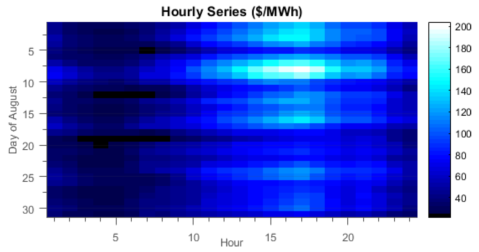
The hourly price series used for August 2007.

Figure 4.
Hourly system operation with Cost-Comfort Particle Swarm Optimization (CCPSO) with two different penalty factors for four days beginning on 8 August 2007.
Figure 4.
Hourly system operation with Cost-Comfort Particle Swarm Optimization (CCPSO) with two different penalty factors for four days beginning on 8 August 2007.

Figure 5.
Cost and comfort when optimizing over August 2007 using five different control strategies. Cost-Comfort Particle Swarm Optimization (CCPSO) finds solutions that simultaneously reduce both discomfort and cost relative to other methods. See text for details on each strategy.
Figure 5.
Cost and comfort when optimizing over August 2007 using five different control strategies. Cost-Comfort Particle Swarm Optimization (CCPSO) finds solutions that simultaneously reduce both discomfort and cost relative to other methods. See text for details on each strategy.


Table 1.
Electricity expenditure, discomfort, and quantity and timing of electricity use during August 2007, for several control strategies with similar comfort levels.
Table 1.
Electricity expenditure, discomfort, and quantity and timing of electricity use during August 2007, for several control strategies with similar comfort levels.
| CCPSO | Brick-Wall PSO | Night Setback | Transactive Power | Linear Building Optimization | |
|---|---|---|---|---|---|
| Parameters used | w = 173 | N/A | 75 °F | k = 3, −0/+10 °F | w = 568 |
| Discomfort index (106 °F2·person·hour) | 4.0 | 4.1 | 4.1 | 2.9 | 4.3 |
| Total electricity cost ($) | 9561 | 9624 | 10,192 | 10,621 | 10,763 |
| Mean air conditioning electrical load (kW) | 166 | 164 | 160 | 171 | 216 |
| Mean load during 5% highest-price hours (kW) | 271 | 279 | 314 | 283 | 219 |
| Mean load during 5% lowest-price hours (kW) | 205 | 178 | 2 | 0 | 269 |
| Mean price for all power used ($/MWh) | 77.4 | 78.7 | 85.8 | 83.3 | 66.9 |
CCPSO: Cost-Comfort Particle Swarm Optimization; PSO: Particle Swarm Optimization.
© 2018 by the authors. Licensee MDPI, Basel, Switzerland. This article is an open access article distributed under the terms and conditions of the Creative Commons Attribution (CC BY) license (http://creativecommons.org/licenses/by/4.0/).
Share and Cite
MDPI and ACS Style
Izawa, A.; Fripp, M. Multi-Objective Control of Air Conditioning Improves Cost, Comfort and System Energy Balance. Energies 2018, 11, 2373. https://doi.org/10.3390/en11092373
AMA Style
Izawa A, Fripp M. Multi-Objective Control of Air Conditioning Improves Cost, Comfort and System Energy Balance. Energies. 2018; 11(9):2373. https://doi.org/10.3390/en11092373
Chicago/Turabian StyleIzawa, Andrew, and Matthias Fripp. 2018. "Multi-Objective Control of Air Conditioning Improves Cost, Comfort and System Energy Balance" Energies 11, no. 9: 2373. https://doi.org/10.3390/en11092373
Note that from the first issue of 2016, this journal uses article numbers instead of page numbers. See further details here.