Numerical Simulation Study on Seepage Theory of a Multi-Section Fractured Horizontal Well in Shale Gas Reservoirs Based on Multi-Scale Flow Mechanisms

Abstract

Aimed at the multi-scale fractures for stimulated reservoir volume (SRV)-fractured horizontal wells in shale gas reservoirs, a mathematical model of unsteady seepage is established, which considers the characteristics of a dual media of matrix and natural fractures as well as flow in the large-scale hydraulic fractures, based on a discrete-fracture model. Multi-scale flow mechanisms, such as gas desorption, the Klinkenberg effect, and gas diffusion are taken into consideration. A three-dimensional numerical model based on the finite volume method is established, which includes the construction of spatial discretization, calculation of average pressure gradient, and variable at interface, etc. Some related processing techniques, such as boundedness processing upstream and downstream of grid flow, was used to limit non-physical oscillation at large-scale hydraulic fracture interfaces. The sequential solution is performed to solve the pressure equations of matrix, natural, and large-scale hydraulic fractures. The production dynamics and pressure distribution of a multi-section fractured horizontal well in a shale gas reservoir are calculated. Results indicate that, with the increase of the Langmuir volume, the average formation pressure decreases at a slow rate. Simultaneously, the initial gas production and the contribution ratio of the desorbed gas increase. With the decrease of the pore size of the matrix, gas diffusion and the Klinkenberg effect have a greater impact on shale gas production. By changing the fracture half-length and the number of fractured sections, we observe that the production process can not only pursue the long fractures or increase the number of fractured sections, but also should optimize the parameters such as the perforation position, cluster spacing, and fracturing sequence. The stimulated reservoir volume can effectively control the shale reservoir.

1. Introduction

As an important part of unconventional oil and gas resources, shale gas resources have become a new hot spot in recent years. At present, numerical simulation models for shale gas mainly include dual media, multiple discrete media, and equivalent media, among which dual media models are widely used. Sawyer and Kucuk [1] first studied the pressure changes of shale gas reservoirs based on a dual-porosity continuous medium. Subsequently, Bumb and McKee [2] studied the effect of adsorption-desorption on transient behaviour by adding additional adsorption coefficients to the Langmuir isotherm equation. However, the above studies ignore the diffusion processes at the nano-microscales. Carlson and Mercer [3] investigated the pressure changes in vertical wells of a shale gas reservoir by introducing diffusion and desorption terms into a dual-porosity media. The model predicts the productivity of shale gas accurately in a short term. However, the long-term prediction of productivity of gas wells is inaccurate, due to the failure to consider the slippage effect. Swami et al. [4] established a dual media model that considers the Knudsen diffusion, slippage, and sorption-desorption processes, and is validated by laboratory data.

Some researchers [5,6,7,8,9,10,11] have pointed out that although dual media models are widely used in commercial software, due to their inherent shortcomings, full or partial encryption still suffers from poor adaptability to multi-scale fracture network systems. In addition, due to the micro-pores in shale gas reservoirs, it is usually necessary to conduct fracturing to obtain a commercial gas production rate. However, natural and artificial fractures have big differences in morphology and seepage ability. Kuuskraa et al. [12] propose to use multiple discrete media models to study the productivity of shale gas reservoirs. Based on the concept of multiple media, Schepers [13] and Dehghanpour et al. [14] established a Darcy flow model that couples diffusion and desorption processes with matrix flow, respectively. Wu et al. [15] established a multi-discrete medium model of dense fractured reservoirs, considering the stress sensitivity and slippage effects of fractures. The fractures are divided into natural micro-fractures and artificial fractures. The slippage effect in the matrix is considered and the differences between the multi-discrete and dual-media models are compared. Aboaba and Cheng [16] used a linear flow model to study the typical productivity curve, which describes changes of fractured horizontal wells in shale gas reservoirs without regard to adsorption and diffusion. In combination with the perturbation method and the point source function, a well test model for a horizontal well, considering diffusion and Darcy flow in a fracture, was proposed by Wang [17]. However, this model does not consider the influence of the reconstructed volume on the pressure change in a horizontal well. Fang et al. [18] considered the compressibility of tight reservoirs and the nonlinear seepage of matrix fluids, and established a multi-scale seepage discrete fracture model of two-dimensional volume fracturing.

In this paper, the authors summarize the law of flow in shale gas reservoirs and establish a three-dimensional (3D) composite model, which uses dual media to describe matrix-natural micro-fractures and utilizes discrete media to describe artificial fractures. The production of multi-section fractured horizontal wells in a rectangular shale gas reservoir is described, considering gas desorption, the Klinkenberg effect, and gas diffusion in the matrix. The stimulated volume is determined by parameter setting of the artificial fractures. The numerical solution is obtained by using the finite volume element method.

2. Mathematical Model

2.1. Assumptions

Figure 1a shows a multi-section fractured horizontal well in a shale gas reservoir. The x–y plane represents the horizontal plane, and the z-axis represents the vertical direction. Artificial fractures are represented by two-dimensional elemental bodies. Segments of the horizontal well are represented by one-dimensional, line-element entities. In order to simplify the model, we propose the following assumptions:

• The gas reservoirs are rectangular, and the flow is an isothermal flow. The gas reservoirs are divided into artificial fractures, natural micro-fractures, and matrix;
• Flows in artificial fractures and natural micro-fractures are described by Darcy’s law. The gas desorption in a matrix pore is described by the Langmuir isotherm equation;
• Horizontal wells produce at constant pressure. There is only a single-phase gas in gas reservoirs;
• The fractures are perpendicular to the horizontal wellbore and symmetrical about the wellbore;
• Permeability anisotropy and gravity effects are ignored, and natural gas can only flow into the horizontal wellbore through artificial fractures;
• Shale gas consists of methane, and does not consider the effect of competitive adsorption on the adsorption-desorption process;
• Gas diffusion process in shale gas matrix is a non-equilibrium, quasi-steady-state process, which obeys Fick’s first law.

2.2. Governing Equation

2.2.1. Flow Equation

According to the real gas state equation, the shale gas density can be defined as

$${\rho }_{\mathrm{gi}}=\frac{M_{\mathrm{g}}{p}_{\mathrm{i}}}{ZRT}$$

(1)

where $\mathrm{i}=\mathrm{m}\mathrm{or}\mathrm{f}$ represents the matrix and the fractures, respectively; ${\rho }_{\mathrm{g}}$ is gas density (kg m⁻³); $M_{\mathrm{g}}$ is the molecular mass (kg mol⁻¹); $Z$ is the gas deviation factor (dimensionless); $p$ is pressure (Pa); $R$ is the universal gas constant (J mol⁻¹ k⁻¹); and $T$ is temperature (K).

Based on the above assumptions, the governing flow equation of shale gas in the matrix can be obtained from the law of conservation of mass, as follows:

$$\frac{\partial \left({\rho }_{\mathrm{gm}}{\varphi }_{\mathrm{m}}\right)}{\partial t}+\nabla \cdot \left({\rho }_{\mathrm{gm}}{v}_{\mathrm{m}}\right)+\left(1-{\varphi }_{\mathrm{m}}\right)q_{\mathrm{m}}+q_{\mathrm{m}-\mathrm{f}}=0$$

(2)

where ${\varphi }_{\mathrm{m}}$ is the shale matrix porosity (value), $v_{\mathrm{m}}$ is the apparent gas velocity (m s⁻¹), $q_{\mathrm{m}}$ is the matrix desorption rate (m³ s⁻¹), and $q_{\mathrm{m}-\mathrm{f}}$ is the crow-flow rate from the matrix to the fracture (m³ s⁻¹).

The first term in the formula represents the change of fluid mass in the unit volume element of the matrix. The second term is the flux flowing through the surface of the element, which must be modified by introducing the shale-gas-transport mechanisms in nanopores. In this paper, we consider gas molecular diffusion, slippage, and desorption. The third term is the desorption capacity of the matrix. The fourth item is the cross-flow from the matrix to the fracture. Generally speaking, water is not able to enter the micro-pores in the matrix of shale gas reservoirs. Therefore, it is reasonable to consider that there is only gas phase in the matrix. In other words, the gas in the micro-pores can be divided into adsorption gas adsorbing on the surface of the matrix and the free gas flowing in the micro-pores.

According to the study by Javadpour [19], the Knudsen number is in the transition zone of the viscous flow and Knudsen diffusion under shale gas formation conditions. At this time, the mass exchange of gas in the matrix is affected by viscous flow, Knudsen diffusion, and desorption. Therefore, corrections should be made to the mass flow in the matrix:

$${\rho }_{\mathrm{gm}}{v}_{\mathrm{m}}={\rho }_{\mathrm{gm}}\left(v_{\mathrm{m}}^{\mathrm{v}}+v_{\mathrm{m}}^{\mathrm{k}}\right)$$

(3)

where $v_{\mathrm{m}}^{\mathrm{v}}$ is the corrected gas velocity considering the Klinkenberg effect, and $v_{\mathrm{m}}^{\mathrm{k}}$ is the corrected gas velocity considering the diffusive transport. The measure of pores in the matrix is usually tiny compared to other reservoir types. The additional contribution of the Klinkenberg effect to gas transport may be due to frequent collisions of gas molecules with the wall of the pores, causing the gas viscosity in the Knudsen layer to gradually deviate from the traditional gas viscosity. According to the study by Karniadakis et al., the gas effective viscosity can be expressed as

$${\mu }_{eff}={\mu }_{\mathrm{g}}\left(\frac{1}{1+8\alpha K_{\mathrm{n}}}\right)$$

(4)

where ${\mu }_{eff}$ is the gas effective viscosity (mPa·s), ${\mu }_{\mathrm{g}}$ is gas viscosity (mPa·s), $\alpha$ is the rarefaction coefficient (dimensionless), and $K_{\mathrm{n}}$ is the Knudsen number (dimensionless).

Combing Equation (4) and Darcy’s law, the corrected gas velocity with the Klinkenberg effect can be expressed as follows:

$$v_{\mathrm{m}}^{\mathrm{v}}=-\frac{k_{\mathrm{m}}}{{\mu }_{\mathrm{g}}}\left(1+8\alpha K_{\mathrm{n}}\right)\nabla p_{\mathrm{m}}$$

(5)

There are two fundamental modes: the advection and diffusion of fluid transport. The flow governing equation usually neglects the diffusive contribution, which is reasonable for most reservoirs—having a medium-high permeability, it may be unreasonable for shale gas. According to the mechanism of fluid dynamics [20], the gas diffusive velocity then can be expressed as

$$v_{\mathrm{m}}^{\mathrm{k}}=-\frac{{\delta }^{\mathrm{m}}}{{\rho }_{\mathrm{gm}}{\tau }^{\mathrm{m}}}{\varphi }_{\mathrm{m}}{D}_{\mathrm{g}}\nabla {\rho }_{\mathrm{gm}}=-\frac{{\delta }^{\mathrm{m}}}{{\rho }_{\mathrm{gm}}{\tau }^{\mathrm{m}}}{\varphi }_{\mathrm{m}}{D}_{\mathrm{g}}\frac{\partial {\rho }_{\mathrm{gm}}}{\partial p_{\mathrm{m}}}\nabla p_{\mathrm{m}}=-\frac{{\delta }^{\mathrm{m}}}{{\tau }^{\mathrm{m}}}{\varphi }_{\mathrm{m}}{c}_{\mathrm{g}}{D}_{\mathrm{g}}\nabla p_{\mathrm{m}}$$

(6)

where $D_{\mathrm{g}}$ is the Knudsen molecule diffusivity (m² s⁻¹), $c_{\mathrm{g}}$ is the gas compression factor (Pa⁻¹; ${\delta }^{\mathrm{m}}$), and ${\tau }^{\mathrm{m}}$ is the constrictivity and tortuosity of the shale matrix, respectively. The value of ${\delta }^{\mathrm{m}}/{\tau }^{\mathrm{m}}$ is always less than one. Therefore, Equation (3) can be rewritten as

$${\rho }_{\mathrm{gm}}{v}_{\mathrm{m}}=-{\rho }_{\mathrm{gm}}\left[\frac{k_{\mathrm{m}}}{{\mu }_{\mathrm{g}}}\left(1+8\alpha K_{\mathrm{n}}\right)+\frac{{\delta }^{\mathrm{m}}}{{\tau }^{\mathrm{m}}}{\varphi }_{\mathrm{m}}{c}_{\mathrm{g}}{D}_{\mathrm{g}}\right]\nabla p_{\mathrm{m}}$$

(7)

Another contribution to gas production from shale reservoirs comes from the desorption of the gas (mostly to the kerogen) absorbed in shale, which is quantified via the change in the gas adsorption amount. The amount of gas adsorption per unit matrix volume at any pressure can be described by the Langmuir isotherm; then, the matrix desorption rate can be expressed as follows

$$q_{\mathrm{m}}=-\frac{\mathrm{d}{V}_{\mathrm{m}}}{\mathrm{d}t}=-\frac{\partial }{\partial t}\left(\frac{{\rho }_{\mathrm{m}}{M}_{\mathrm{g}}}{V_{\mathrm{std}}}\frac{V_{\mathrm{L}}{p}_{\mathrm{m}}}{p_{\mathrm{L}}+p_{\mathrm{m}}}\right)$$

(8)

where $V_{\mathrm{m}}$ is the adsorption capacity of per unit volume matrix (m³), $V_{\mathrm{L}}$ is the Langmuir volume (m³ kg⁻¹), $p_{\mathrm{L}}$ is the Langmuir pressure (Pa), and $V_{\mathrm{std}}$ is the mole volume of gas at temperature (273.15 K) and pressure (101,325 Pa).

Substitute Equations (1), (5), (6) and (8) into Equation (2), the governing equation for gas transport in the shale matrix is given by

$$\begin{array}{l}\nabla \left\{\left[\frac{k_{\mathrm{m}}}{{\mu }_{\mathrm{g}}}\left(1+8\alpha K_{\mathrm{n}}\right)+\frac{{\delta }^{\mathrm{m}}}{{\tau }^{\mathrm{m}}}{\varphi }_{\mathrm{m}}{c}_{\mathrm{g}}{D}_{\mathrm{g}}\right]\frac{M_{\mathrm{g}}{p}_{\mathrm{m}}}{ZRT}\nabla p_{\mathrm{m}}\right\}-{\sigma }_1\frac{k_{\mathrm{m}}}{{\mu }_{\mathrm{g}}}\frac{M_{\mathrm{g}}{p}_{\mathrm{m}}}{ZRT}\left(p_{\mathrm{m}}-p_{\mathrm{f}}\right)\\ ={\varphi }_{\mathrm{m}}\frac{M_{\mathrm{g}}}{ZRT}\frac{\partial p_{\mathrm{m}}}{\partial t}+\left(1-{\varphi }_{\mathrm{m}}\right)\frac{\partial }{\partial t}\left(\frac{{\rho }_{\mathrm{m}}{M}_{\mathrm{g}}}{V_{\mathrm{std}}}\frac{V_{\mathrm{L}}{p}_{\mathrm{m}}}{p_{\mathrm{L}}+p_{\mathrm{m}}}\right)\end{array}$$

(9)

Analogously, for natural micro-fractures systems:

$$\frac{{\varphi }_{\mathrm{f}}{M}_{\mathrm{g}}}{ZRT}\frac{\partial p_{\mathrm{f}}}{\partial t}-\nabla \cdot \left(\frac{M_{\mathrm{g}}{p}_{\mathrm{f}}}{ZRT}\frac{k_{\mathrm{f}}}{{\mu }_{\mathrm{g}}}\nabla p_{\mathrm{f}}\right)-{\sigma }_1\frac{k_{\mathrm{m}}}{{\mu }_{\mathrm{g}}}\frac{M_{\mathrm{g}}{p}_{\mathrm{m}}}{ZRT}\left(p_{\mathrm{m}}-p_{\mathrm{f}}\right)+q_{\mathrm{f}-\mathrm{h}}=0$$

(10)

where $q_{\mathrm{f}-\mathrm{h}}$ is the crow-flow rate from the natural micro-fracture to the artificial fracture (m³s⁻¹). For artificial fractures system

$$d_{\mathrm{hf}}\frac{\partial \left({\rho }_{\mathrm{g}}{\varphi }_{\mathrm{hf}}\right)}{\partial t}-\frac{\partial }{\partial l}\cdot \left(d_{\mathrm{hf}}\frac{{\rho }_{\mathrm{g}}{k}_{\mathrm{hf}}}{{\mu }_{\mathrm{g}}}\frac{\partial p_{\mathrm{hf}}}{\partial l}\right)-\left(q_{\mathrm{f}-\mathrm{h}}-q_{\mathrm{well}}\right)=0$$

(11)

where $q_{\mathrm{well}}$ is the horizontal well productivity (m³ s⁻¹).

2.2.2. Initial Conditions

Under the initial conditions, the whole formation pressure is the original formation pressure, so

$${p_{\mathrm{m}}\left(x,y,z,t\right)|}_{t=0}={p_{\mathrm{f}}\left(x,y,z,t\right)|}_{t=0}={p_{\mathrm{hf}}\left(x,y,z,t\right)|}_{t=0}=p_{\mathrm{i}}$$

2.2.3. Boundary Conditions

${\Gamma }_{\mathrm{out}}$ represents the outside boundary, and ${\Gamma }_{\mathrm{in}}$ represents the inner boundary. It is assumed that the outer boundary of the model is the sealed boundary, and the production well produces at constant pressure. In that case, the well has the boundary conditions as follows:

$$\begin{array}{l}{\frac{\partial p}{\partial n}|}_{{\Gamma }_{\mathrm{out}}}=0\\ {p|}_{{\Gamma }_{\mathrm{in}}}=p_{\mathrm{wf}}\end{array}$$

3. Discretization and Numerical Solution

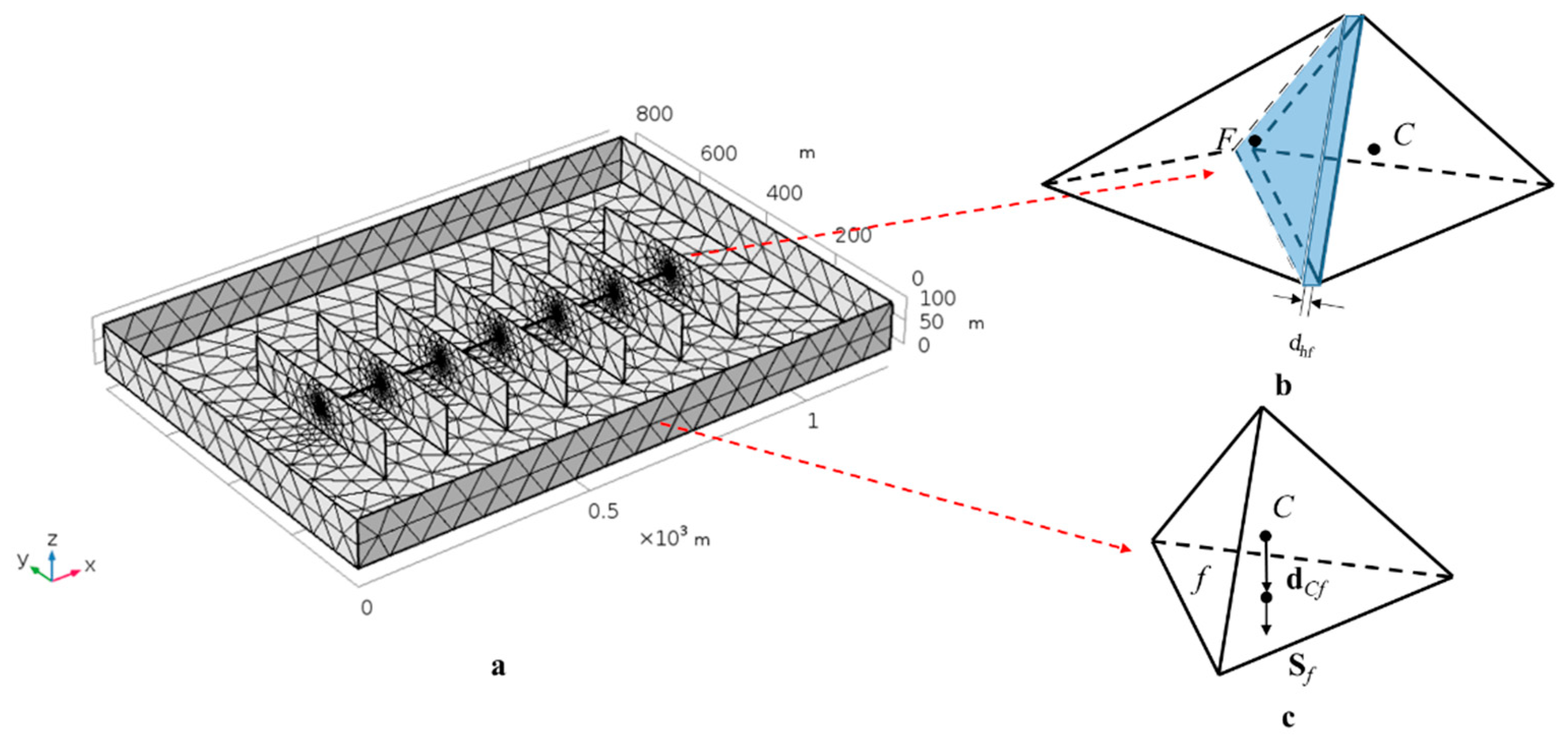
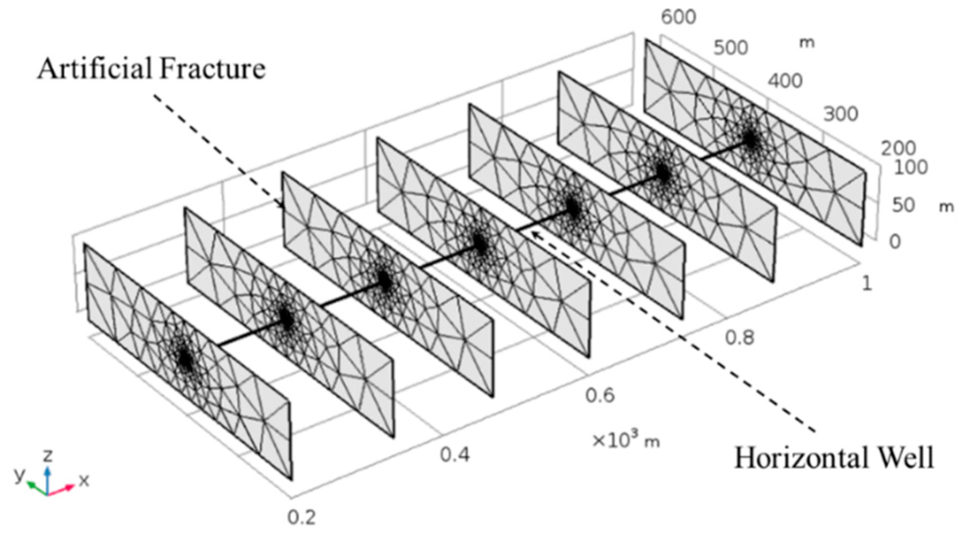
3.1. Domain Discretization

Due to the geometric center coinciding with the centroid of the tetrahedral grid, in order to simplify the calculation, the whole reservoir region is discretized by the unstructured tetrahedron. Other types of grids are needed to recalculate the centroid of the control volume. As shown in Figure 1c, the matrix and micro-fracture system are expressed as a tetrahedron grid, considered as a dual continuous medium; the two-dimensional (2D) blue plane is decomposed in tetrahedral elements that are faces of the tetrahedron surrounding the artificial fracture interface, as shown in Figure 1b. Caumon G et al. [21] pointed out that fracture dimension reduction is a key method to improve the convergence of multi-scale simulation calculation. If the fracture is considered as three-dimensional, a large number of minimized grids will be generated, which will cause the subsequent calculations to fail to converge. The research of Juanes et al. [22] shows that the convergence of the two dimensions is significantly improved by considering the fracture in two dimensions. In addition, as shown in Figure 1c, unlike the traditional finite element method, we establish controlling volume on each grid to obtain the cell-centroid finite volume numerical calculation format. The computational domain ${\Gamma }_{\mathrm{d}}$ consists of two subdomains: ${\Gamma }_{\mathrm{m}-\mathrm{f}}$ representing the matrix and micro-fractures system, and ${\Gamma }_{\mathrm{hf}}$ representing the artificial fractures system. In this paper, FGE is used to represent the flow governing equation. Therefore, the integration of the entire domain ${\Gamma }_{\mathrm{d}}$ can be written as

$${\displaystyle \underset{{\Gamma }_{\mathrm{d}}}{\iiint }\mathrm{FGEd}{\Gamma }_{\mathrm{d}}={\displaystyle \underset{{\Gamma }_{\mathrm{m}-\mathrm{f}}}{\iiint }\mathrm{FGEd}{\Gamma }_{\mathrm{m}-\mathrm{f}}}}+{\mathrm{d}}_{\mathrm{hf}}\times {\displaystyle \underset{{\Gamma }_{\mathrm{hf}}}{\iiint }\mathrm{FGEd}{\Gamma }_{\mathrm{hf}}}$$

(12)

As shown in Figure 2a, different from the vertex-centered variable arrangement in conventional finite element methods, this paper uses a cell-centered variable arrangement to define a control volume. As shown in Figure 2b, in a vertex-centered arrangement the flow variables are stored at the vertices, with elements constructed around the variables’ locations.

Compared with vertex-centered variable arrangement, the cell-centered variable arrangement yields a high order accuracy of integrations. Moreover, it decreases the storage requirements. Furthermore, there is no additional treatment on the boundary to ensure a consistent solution. Another major advantage is that there is no need to pre-define a shape function based on element types.

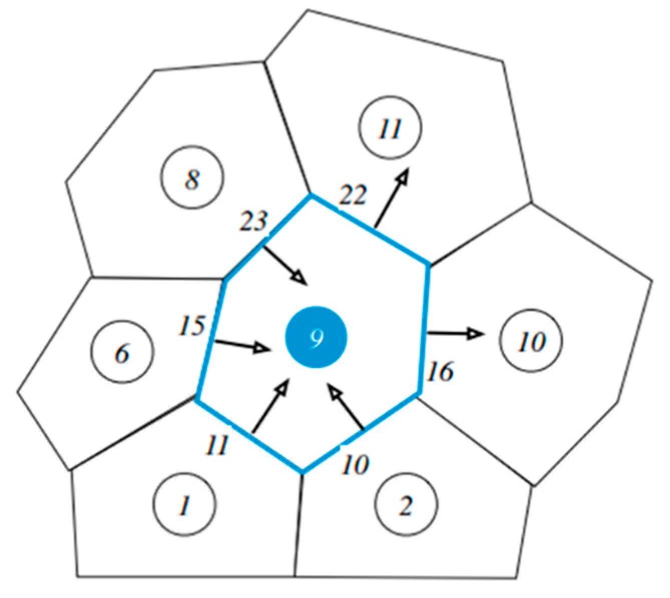
3.2. Equation Discretization

This section uses the matrix system flow governing equation as an example to illustrate the equation discretization process in a tetrahedral mesh. Flow governing equations in micro-fractures and artificial fractures are similar. The process starts by integrating Equation (9) over element C, which enables the recovery of its integral balance, as

$$\begin{array}{l}{\displaystyle \underset{V_{\mathrm{c}}}{\int }{\varphi }_{\mathrm{m}}\frac{M_{\mathrm{g}}}{ZRT}\frac{\partial p_{\mathrm{m}}}{\partial t}\mathrm{d}V}-{\displaystyle \underset{V_{\mathrm{c}}}{\int }\nabla \left\{\left[\frac{k_{\mathrm{m}}}{{\mu }_{\mathrm{g}}}\left(1+8\alpha K_{\mathrm{n}}\right)+\frac{{\delta }^{\mathrm{m}}}{{\tau }^{\mathrm{m}}}{\varphi }_{\mathrm{m}}{c}_{\mathrm{g}}{D}_{\mathrm{g}}\right]\frac{M_{\mathrm{g}}{p}_{\mathrm{m}}}{ZRT}\nabla p_{\mathrm{m}}\right\}}\mathrm{d}V\\ +{\displaystyle \underset{V_{\mathrm{c}}}{\int }\left(1-{\varphi }_{\mathrm{m}}\right)\frac{\partial }{\partial t}\left(\frac{{\rho }_{\mathrm{m}}{M}_{\mathrm{g}}}{V_{\mathrm{std}}}\frac{V_{\mathrm{L}}{p}_{\mathrm{m}}}{p_{\mathrm{L}}+p_{\mathrm{m}}}\right)}\mathrm{d}V+{\displaystyle \underset{V_{\mathrm{c}}}{\int }{\sigma }_1\frac{k_{\mathrm{m}}}{{\mu }_{\mathrm{g}}}\frac{M_{\mathrm{g}}{p}_{\mathrm{m}}}{ZRT}\left(p_{\mathrm{m}}-p_{\mathrm{f}}\right)}\mathrm{d}V=0\end{array}$$

(13)

The above formula shows that for any control volume, the change of gas mass flux in the matrix system within a certain time period is equal to the sum of the outflow through the control volume, as well as the desorption gas volume and the cross-flow rate, thus ensuring that the model still respects the conservation of mass in any local region. For the sake of mathematical simplicity, the following variable is chosen to be the apparent permeability of shale matrix:

$$\kappa =\frac{k_{\mathrm{m}}}{{\mu }_{\mathrm{g}}}\left(1+8\alpha K_{\mathrm{n}}\right)+\frac{{\delta }^{\mathrm{m}}}{{\tau }^{\mathrm{m}}}{\varphi }_{\mathrm{m}}{c}_{\mathrm{g}}{D}_{\mathrm{g}}$$

(14)

Then, according to the divergence theorem, the volume integral of the advective-diffusive term in Equation (13) is transformed into a surface integral, yielding

$${\displaystyle \underset{V_{\mathrm{c}}}{\int }\nabla \left(\kappa \frac{M_{\mathrm{g}}{p}_{\mathrm{m}}}{ZRT}\nabla p_{\mathrm{m}}\right)}\mathrm{d}V={\displaystyle \underset{\partial V_{\mathrm{c}}}{\oint }\left(\kappa \frac{M_{\mathrm{g}}{p}_{\mathrm{m}}}{ZRT}\nabla p_{\mathrm{m}}\cdot n\right)\mathrm{dS}}$$

(15)

In the presence of discrete faces, the surface integral in Equation (15) becomes

$${\displaystyle \underset{\partial V_{\mathrm{c}}}{\oint }\left(\kappa \frac{M_{\mathrm{g}}{p}_{\mathrm{m}}}{ZRT}\nabla p_{\mathrm{m}}\cdot n\right)\mathrm{dS}}={\displaystyle \sum _{f~faces\left(V_{\mathrm{C}}\right)}\left[{\displaystyle \underset{f}{\int }\left(\kappa \frac{M_{\mathrm{g}}{p}_{\mathrm{m}}}{ZRT}\nabla p_{\mathrm{m}}\cdot n\right)\mathrm{dS}}\right]}$$

(16)

where f is the integral point at the centroid of the boundary surface. Therefore, the integral in Equation (16) is numerically approximated to the flux at the centroids of the faces, which is a second-order approximation.

According to the trapezoidal integral formula, the surface integral in Equation (16) can be written as

$${\displaystyle \underset{f}{\int }\left(\kappa \frac{M_{\mathrm{g}}{p}_{\mathrm{m}}{k}_{\mathrm{m}}}{ZRT{\mu }_{\mathrm{g}}}\nabla p_{\mathrm{m}}\cdot n\right)\mathrm{dS}}\approx \kappa \frac{M_{\mathrm{g}}{p}_{\mathrm{m}}{k}_{\mathrm{m}}}{ZRT{\mu }_{\mathrm{g}}}\nabla p_{\mathrm{m}}\cdot S_f$$

(17)

Therefore, the advective-diffusive term in Equation (13) can be written as

$${\displaystyle \underset{V_{\mathrm{c}}}{\int }\nabla \cdot \left(\kappa \frac{M_{\mathrm{g}}{p}_{\mathrm{m}}{k}_{\mathrm{m}}}{ZRT{\mu }_{\mathrm{g}}}\nabla p_{\mathrm{m}}\right)}\mathrm{d}V={\displaystyle \sum _{f~faces\left(V_{\mathrm{C}}\right)}\left[\left(\kappa \frac{M_{\mathrm{g}}{p}_{\mathrm{m}}}{ZRT}{\lambda }_{\mathrm{m}}\nabla p_{\mathrm{m}}\right)\cdot S_f\right]}$$

(18)

Similarly, the finite volume numerical calculation format for the unsteady term, gas desorption term, and the cross-flow term can be obtained as

$${\displaystyle \underset{V_{\mathrm{c}}}{\int }{\varphi }_{\mathrm{m}}\frac{M_{\mathrm{g}}}{ZRT}\frac{\partial p_{\mathrm{m}}}{\partial t}\mathrm{d}V}=V_{\mathrm{c}}{\varphi }_{\mathrm{m}}\frac{M_{\mathrm{g}}}{ZRT}\frac{\partial p_{\mathrm{m}}}{\partial t}$$

(19)

$${\displaystyle \underset{V_{\mathrm{c}}}{\int }\left(1-{\varphi }_{\mathrm{m}}\right)\frac{\partial }{\partial t}\left(\frac{{\rho }_{\mathrm{m}}{M}_{\mathrm{g}}}{V_{\mathrm{std}}}\frac{V_{\mathrm{L}}{p}_{\mathrm{m}}}{p_{\mathrm{L}}+p_{\mathrm{m}}}\right)}\mathrm{d}V=V_{\mathrm{c}}\left(1-{\varphi }_{\mathrm{m}}\right)\frac{\partial }{\partial t}\left(\frac{{\rho }_{\mathrm{m}}{M}_{\mathrm{g}}}{V_{\mathrm{std}}}\frac{V_{\mathrm{L}}{p}_{\mathrm{m}}}{p_{\mathrm{L}}+p_{\mathrm{m}}}\right)$$

(20)

$${\displaystyle \underset{V_{\mathrm{c}}}{\int }{\sigma }_1\frac{k_{\mathrm{m}}}{{\mu }_{\mathrm{g}}}\frac{M_{\mathrm{g}}{p}_{\mathrm{m}}}{ZRT}\left(p_{\mathrm{m}}-p_{\mathrm{f}}\right)}\mathrm{d}V=V_{\mathrm{c}}{\sigma }_1\frac{k_{\mathrm{m}}}{{\mu }_{\mathrm{g}}}\frac{M_{\mathrm{g}}{p}_{\mathrm{m}}}{ZRT}\left(p_{\mathrm{m}}-p_{\mathrm{f}}\right)$$

(21)

Since the capacity of the desorbed gas is a function of time, then according to Equation (2), the finite volume numerical calculation format of the flow governing equation in the matrix system can be rewritten as:

$$\begin{array}{l}\left[\frac{V_c{\varphi }_{\mathrm{m}}{M}_{\mathrm{g}}}{ZRT}-V_{\mathrm{c}}\left(1-{\varphi }_{\mathrm{m}}\right)\frac{\mathrm{d}{V}_{\mathrm{m}}}{\mathrm{d}{p}_{\mathrm{m}}}\right]\frac{\partial p_{\mathrm{m}}}{\partial t}-{\displaystyle \sum _{f~faces\left(V_{\mathrm{C}}\right)}\left(\kappa \frac{M_{\mathrm{g}}{p}_{\mathrm{m}}}{ZRT}\nabla p_{\mathrm{m}}\right)\cdot S_f}\\ +V_{\mathrm{c}}{\sigma }_1\frac{k_{\mathrm{m}}}{{\mu }_{\mathrm{g}}}\frac{M_{\mathrm{g}}{p}_{\mathrm{m}}}{ZRT}\left(p_{\mathrm{m}}-p_{\mathrm{f}}\right)=0\end{array}$$

(22)

Similarly, the finite volume numerical calculation format for micro-fractures and artificial fractures can be obtained as

$$\frac{V_c{\varphi }_{\mathrm{f}}{M}_{\mathrm{g}}}{ZRT}\frac{\partial p_{\mathrm{f}}}{\partial t}-{\displaystyle \sum _{f~faces\left(V_{\mathrm{C}}\right)}\left(\frac{M_{\mathrm{g}}{p}_{\mathrm{f}}}{ZRT}{\lambda }_{\mathrm{f}}\nabla p_{\mathrm{f}}\right)\cdot S_f}-V_{\mathrm{c}}\left(q_{\mathrm{m}-\mathrm{f}}-q_{\mathrm{f}-\mathrm{h}}\right)=0$$

(23)

$$\begin{array}{l}{d}_{\mathrm{hf}}\left({\displaystyle \sum _{f~faces\left(V_{\mathrm{C}}-\mathrm{F}\right)}\frac{{\mathrm{S}}_f{\varphi }_{\mathrm{hf}}{M}_{\mathrm{g}}}{ZRT}}\right)\frac{\partial p_{\mathrm{hf}}}{\partial t}\\ -d_{\mathrm{hf}}{\displaystyle \sum _{f~faces\left(V_{\mathrm{C}}\right)}{\displaystyle \sum _{b~bounds\left(f\right)}\left(\frac{M_{\mathrm{g}}{p}_{\mathrm{hf}}}{ZRT}{\lambda }_{\mathrm{hf}}\nabla p_{\mathrm{hf}}\right)\cdot S_{\mathrm{b}}}}-V_{\mathrm{c}}\left(q_{\mathrm{f}-\mathrm{h}}-q_{\mathrm{well}}\right)=0\end{array}$$

(24)

3.3. Sequential Solution

The so-called sequential solution method means that each time step solves a variable firstly, and then it substitutes other variables expressions for an iterative solution. This method ensures that the amount of calculation is less than the overall solution method at each time step. Assuming that the current time step is k, then all variables related to the pressure of artificial fractures and matrix are implicitly solved using value at k + 1 time steps. Equations (22) and (24) can be written as:

$$\begin{array}{l}\left[\frac{V_c{\varphi }_{\mathrm{m}}{M}_{\mathrm{g}}}{ZRT}-V_{\mathrm{c}}\left(1-{\varphi }_{\mathrm{m}}\right)\frac{\mathrm{d}{V}_{\mathrm{m}}}{\mathrm{d}{p}_{\mathrm{m}}}\right]\frac{p_{\mathrm{m}}^{\mathrm{k}+1}-p_{\mathrm{m}}^{\mathrm{k}}}{\Delta t}={\displaystyle \sum _{f~faces\left(V_{\mathrm{C}}\right)}\left({\kappa }^{\mathrm{k}+1}\frac{M_{\mathrm{g}}{p}_{\mathrm{m}}^{\mathrm{k}+1}}{ZRT}\nabla p_{\mathrm{m}}^{\mathrm{k}+1}\right)\cdot S_f}\\ -V_{\mathrm{c}}{\sigma }_1{\lambda }_{\mathrm{m}}^{\mathrm{k}+1}\frac{M_{\mathrm{g}}{p}_{\mathrm{m}}^{\mathrm{k}+1}}{ZRT}\left(p_{\mathrm{m}}^{\mathrm{k}+1}-p_{\mathrm{f}}^{\mathrm{k}}\right)=0\end{array}$$

(25)

$$\begin{array}{l}{d}_{\mathrm{hf}}\left({\displaystyle \sum _{f~faces\left(V_{\mathrm{C}}-\mathrm{F}\right)}\frac{{\mathrm{S}}_f{\varphi }_{\mathrm{hf}}{M}_{\mathrm{g}}}{ZRT}}\right)\frac{p_{\mathrm{hf}}^{\mathrm{k}+1}-p_{\mathrm{hf}}^{\mathrm{k}}}{\Delta t}=\\ d_{\mathrm{hf}}{\displaystyle \sum _{f~faces\left(V_{\mathrm{C}}\right)}{\displaystyle \sum _{b~bounds\left(f\right)}\left(\frac{M_{\mathrm{g}}{p}_{\mathrm{hf}}^{\mathrm{k}+1}}{ZRT}{\lambda }_{\mathrm{hf}}^{\mathrm{k}+1}\nabla p_{\mathrm{hf}}^{\mathrm{k}+1}\right)\cdot S_{\mathrm{b}}}}+V_{\mathrm{c}}{\lambda }_{\mathrm{f}}^{\mathrm{k}+1}\left(p_{\mathrm{f}}^{\mathrm{k}}-p_{\mathrm{hf}}^{\mathrm{k}+1}\right)-V_{\mathrm{c}}{q}_{\mathrm{well}}^{\mathrm{k}}\end{array}$$

(26)

Note that in the two expressions, $p_{\mathrm{f}}$ and $q_{\mathrm{well}}$ uses the value of the k time step—these are known values. Therefore, each of the two formulae contains an unknown variable $p_{\mathrm{hf}}^{\mathrm{k}+1}$ and $p_{\mathrm{m}}^{\mathrm{k}+1}$. Therefore, we can iteratively solve the equation using the Newton–Raphson method. Then we substitute the results into the micro-fracture flow governing equation to solve $p_{\mathrm{f}}^{\mathrm{k}+1}$ explicitly.

$$\begin{array}{l}\frac{V_c{\varphi }_{\mathrm{f}}{M}_{\mathrm{g}}}{ZRT}\frac{p_{\mathrm{f}}^{\mathrm{k}+1}-p_{\mathrm{f}}^{\mathrm{k}}}{\Delta t}={\displaystyle \sum _{f~faces\left(V_{\mathrm{C}}\right)}\left(\frac{M_{\mathrm{g}}{p}_{\mathrm{f}}^{\mathrm{k}}}{ZRT}{\lambda }_{\mathrm{f}}^{\mathrm{k}}\nabla p_{\mathrm{f}}^{\mathrm{k}}\right)\cdot S_f}\\ +V_{\mathrm{c}}{\sigma }_1{\lambda }_{\mathrm{m}}^{\mathrm{k}+1}\frac{M_{\mathrm{g}}{p}_{\mathrm{m}}^{\mathrm{k}+1}}{ZRT}\left(p_{\mathrm{m}}^{\mathrm{k}+1}-p_{\mathrm{f}}^{\mathrm{k}}\right)-V_{\mathrm{c}}{\sigma }_2{\lambda }_{\mathrm{f}}^{\mathrm{k}}\frac{M_{\mathrm{g}}{p}_{\mathrm{f}}^{\mathrm{k}}}{ZRT}\left(p_{\mathrm{f}}^{\mathrm{k}}-p_{\mathrm{hf}}^{\mathrm{k}+1}\right)\end{array}$$

(27)

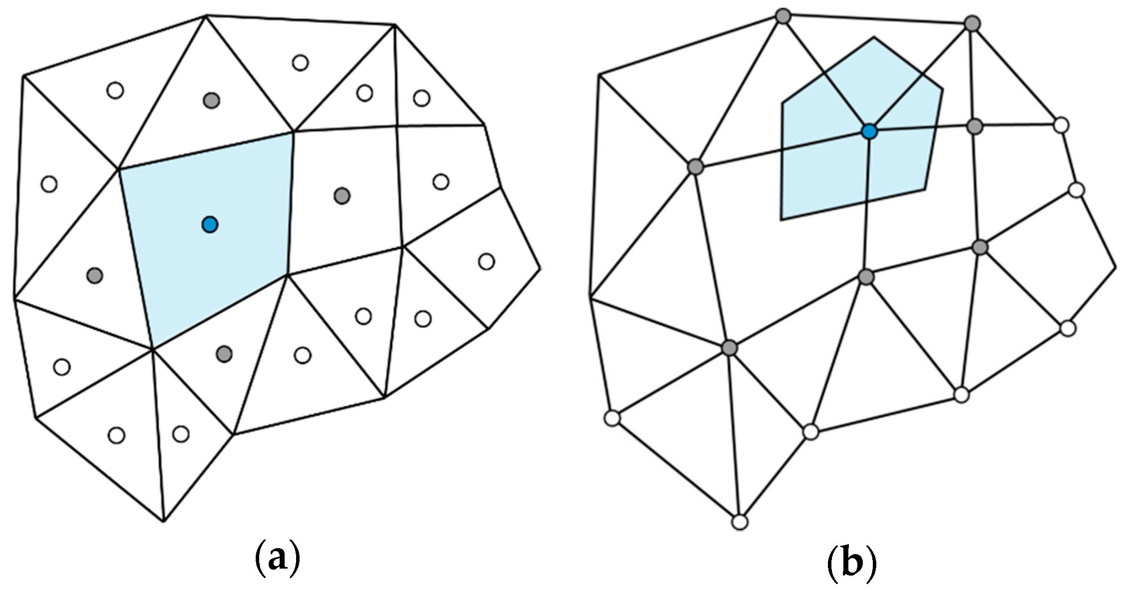
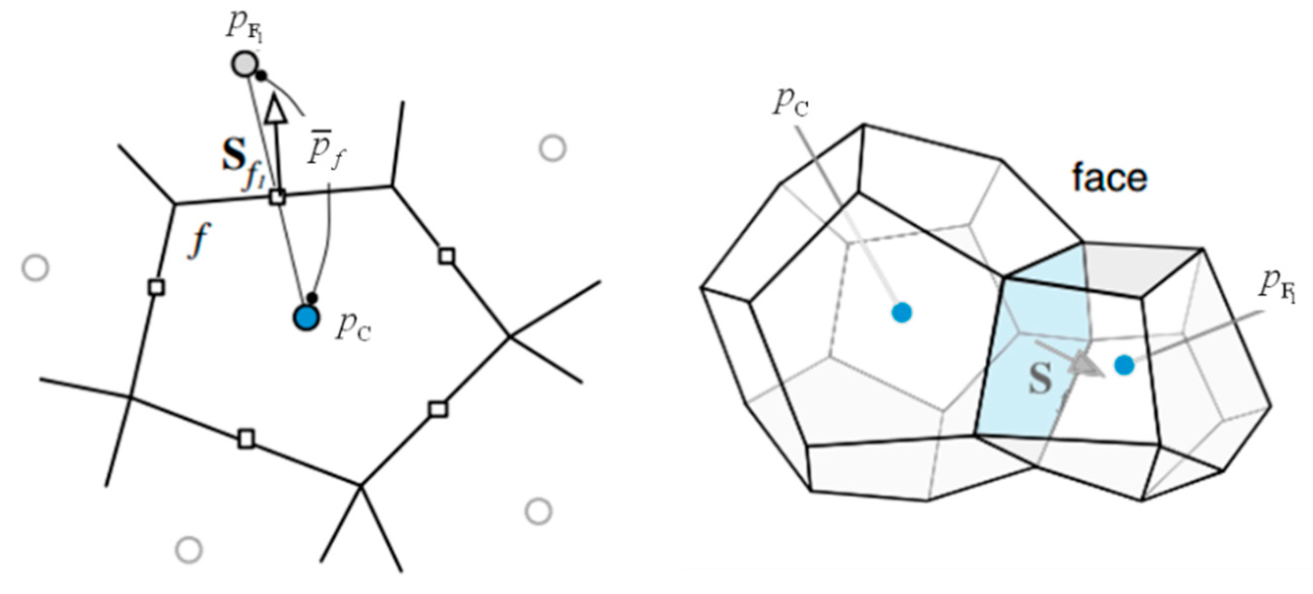
3.4. Gradient Computation

Obviously, to solve Equations (25)–(27), we need to calculate the gradient of an element field. The method adopted in this section is based on the Green-Gauss theorem, which is proven by Cengel [23] and Incropera [24] relatively straightforwardly and can be used for a variety of topologies and girds (structured/unstructured, orthogonal/non-orthogonal, etc.). The starting point is used to define the average pressure gradient over a finite volume element, as shown as Figure 3, of centroid $C$ and volume $V_{\mathrm{C}}$:

$${\overline{\nabla p}}_{\mathrm{c}}=\frac{1}{V_{\mathrm{c}}}{\displaystyle \underset{V_{\mathrm{c}}}{\int }\nabla pdV}$$

(28)

Then, using the divergence theorem, the volume integral is transformed into the surface integral

$${\overline{\nabla p}}_{\mathrm{c}}=\frac{1}{V_{\mathrm{c}}}{\displaystyle \underset{\partial V_{\mathrm{c}}}{\int }p\mathrm{d}S}$$

(29)

where $\mathrm{d}S$ is the surface vector pointing outward. In the case of discrete faces, Equation (29) can be rewritten as

$${\overline{\nabla p}}_{\mathrm{c}}{V}_{\mathrm{c}}={\displaystyle \sum _{\partial V_{\mathrm{c}}}{\displaystyle \underset{face}{\int }p\mathrm{d}S}}$$

(30)

Next, the integral of a cell face is approximated by the mid-point integration rule, which is equal to the interpolated value of the field at the face centroid multiplied by the face area, resulting in

$${\overline{\nabla p}}_{\mathrm{c}}=\frac{1}{V_{\mathrm{c}}}{\displaystyle \sum _{f=nb\left(C\right)}{\overline{p}}_f{S}_f}$$

(31)

By reviewing Equations (30) and (31) in Figure 3, it is apparent that to calculate the average pressure gradient of the control element $C$, the information about the surface vector ($S_f$) is needed, as well as information about the adjacent elements and the pressure values at the element centroids ($p_{\mathrm{C}}$, $p_{{\mathrm{F}}_{\mathrm{k}}}$). This information is needed to calculate the pressure at the interface ($p_f$), which must be interpolated in some way.

Assuming that the pressure between the elements $C$ and $F$ straddling the interface $f$ varies linearly, the approximate value for $p_f$, denoted by ${\overline{p}}_f$, can be calculated as

$${\overline{p}}_f=g_F{p}_F+g_C{p}_C$$

(32)

Calculation of the weight factors $g_F$ and $g_C$ is given by

$$g_F=\frac{V_C}{V_C+V_F}{g}_C=\frac{V_F}{V_C+V_F}=1-g_F$$

(33)

Figure 4 considers the straddling elements; the surface vector cannot be outward at the same time, so the direction of the surface vector defined for this grid is determined by the grid index. The direction of the surface vector always points from the element which has a smaller index number to the element has a larger index number. In order to consider the vector direction, use a sign function to modify Equation (31) for the gradient as

$${\overline{\nabla p}}_{\mathrm{k}}=\frac{1}{V_{\mathrm{k}}}\left(-{\displaystyle \sum _{\mathrm{n}\leftarrow \langle f=nb\left(C\right)\rangle <\mathrm{k}}{\overline{p}}_{\mathrm{n}}{\mathrm{S}}_{\mathrm{n}}}+{\displaystyle \sum _{\mathrm{n}\leftarrow \langle f=nb\left(C\right)\rangle >\mathrm{k}}{\overline{p}}_{\mathrm{n}}{\mathrm{S}}_{\mathrm{n}}}\right)$$

(34)

3.5. Non-Orthogonality

Due to the non-structural grid used in this article, the grids are non-orthogonal. Therefore, the surface vector $S_f$ and the vector $CF$ connects the centroids of the elements, which straddle the interface and are not collinear. In this case, the pressure gradient perpendicular to the surface cannot be written as a function of $p_{\mathrm{C}}$ and $p_{\mathrm{F}}$, because it has a component in the direction perpendicular to $CF$.

If $e$ represents the unit vector along the direction defined by the vector $CF$, then the pressure gradient in the $e$ direction can be written as

$${\left(\nabla p\cdot e\right)}_f={\left(\frac{\partial p}{\partial e}\right)}_f=\frac{p_{\mathrm{F}}-p_{\mathrm{C}}}{\Vert r_{\mathrm{F}}-r_{\mathrm{C}}\Vert }=\frac{p_{\mathrm{F}}-p_{\mathrm{C}}}{d_{\mathrm{CF}}}$$

(35)

Thus, to achieve the linearization of the flux in non-orthogonal grids, the surface vector $S_f$ should be written as the sum of two vectors $E_f$ and $T_f$, i.e.,

$$S_f=E_f+T_f$$

(36)

where $E_f$ is in the $CF$ direction, such that part of the diffusion flux through face f can be written as a function of the nodal values $p_{\mathrm{C}}$ and $p_{\mathrm{F}}$:

$$\begin{array}{ll}{\left(\nabla p\right)}_f\cdot S_f& ={\left(\nabla p\right)}_f\cdot E_f+{\left(\nabla p\right)}_f\cdot T_f\\ & =E_f{\left(\frac{\partial p}{\partial e}\right)}_f+{\left(\nabla p\right)}_f\cdot T_f\\ & =E_f\frac{p_F-p_C}{d_{\mathrm{CF}}}+{\left(\nabla p\right)}_f\cdot T_f\end{array}$$

(37)

Some researchers [25,26,27] give different options for the decomposition of $S_f$, which are shown in

Table 1. Different options for the decomposition of surface vector $S_f$.

Option	Diagram	$E_f$	$T_f$
Minimum Correction Approach		Ef = (e·Sf)e = (Sfcosθ)e	Tf = (n − cosθe)Sf
Orthogonal Correction Approach		Ef = Sfe	Tf = (n − e)Sf
Over-Relaxed Approach		$E_f=\left(\frac{S_f}{\cos \theta }\right)\mathbf{e}$	$T_f=(\mathbf{n}-\frac{1}{\cos \theta }\mathbf{e})S_f$

.

The above methods are correct and satisfy Equation (9). These methods differ in their accuracy and stability on non-orthogonal grids. It has been found that the over-relaxed approach is the most stable, even when the grid is highly non-orthogonal.

Minimum Correction Approach

$$\begin{gathered} T_f=\left(n-\cos \theta e\right)S_f \\ {E}_f=S_{f}e \end{gathered}$$

Orthogonal Correction Approach

$$\begin{gathered} T_f=\left(n-e\right)S_f \\ {E}_f=\left(\frac{S_f}{\cos \theta }\right)e \end{gathered}$$

Over-Relaxed Approach

$$T_f=\left(n-\frac{1}{\cos \theta }e\right)S_f$$

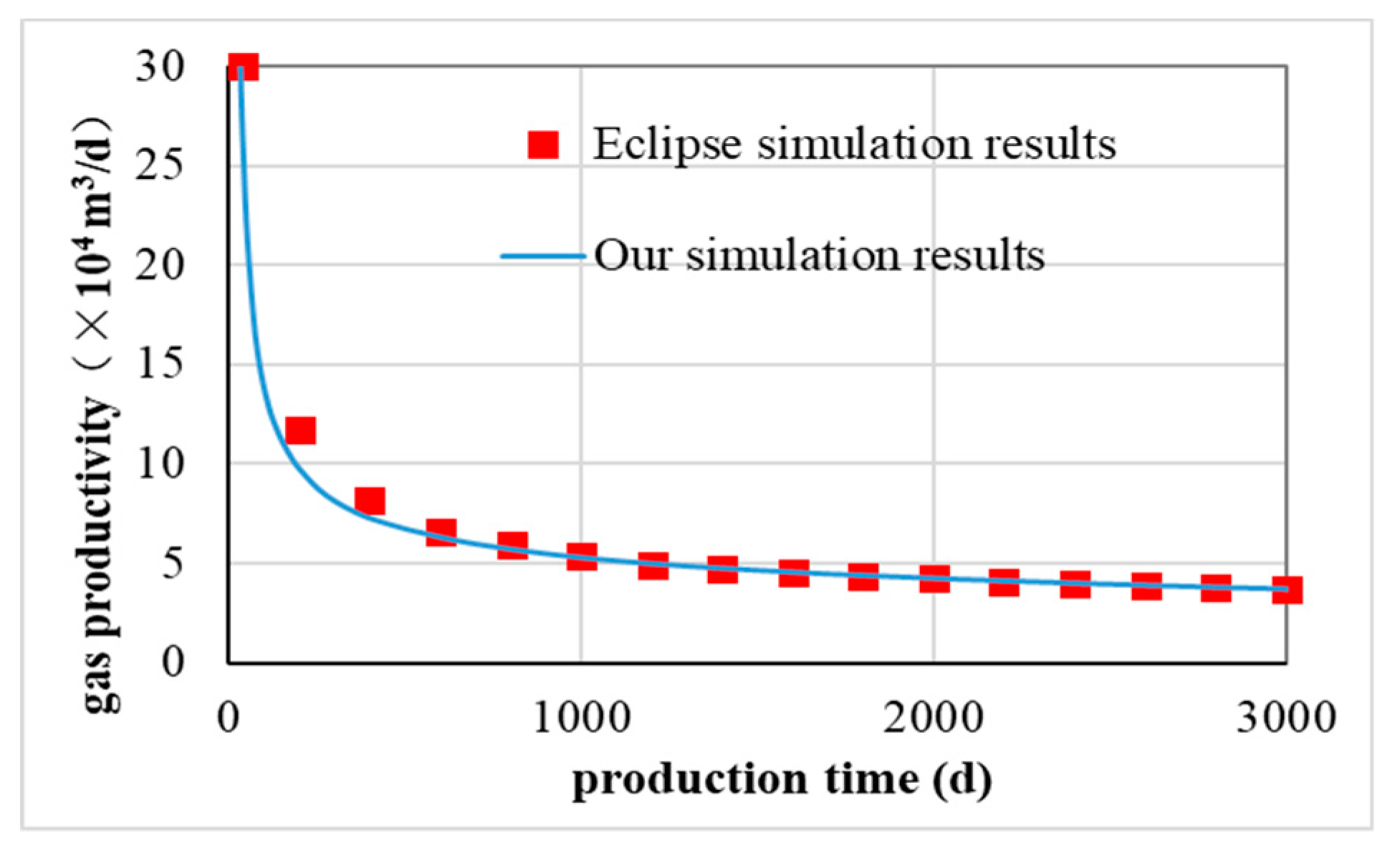
3.6. Model Verification

In this paper, a rectangular composite shale gas reservoir model considering a finite-conductivity fractured horizontal well is established. If the multi-scale flow mechanisms and the hydraulic fractures (SRV) region are ignored, the model can be applied to the multi-section fractured horizontal well of conventional dual-porosity gas reservoirs. To verify the accuracy of this method, comparisons are made with the solution using commercial software Eclipse [28]. Both simulations are applied for an 800 m long horizontal well with fifteen equally-spaced 200 m long transverse fractures in a bounded rectangular conventional reservoir. The data for the formation and well properties used in the simulations are shown in

Table 2. Basic data of a multi-section fractured horizontal well in a single-porosity gas reservoir [27].

Parameter	Unit	Value
Reservoir length	m	2000
Reservoir width	m	2000
Reservoir height	m	50
Horizontal well length	m	800
Artificial fracture height	m	40
Wellbore radius,$r_{\mathrm{w}}$	m	0.1
Matrix permeability, $k_{\mathrm{m}}$	mD	0.5
Matrix porosity, ${\varphi }_{\mathrm{m}}$	-	0.05
Artificial fracture number	-	15
Artificial fracture length, $l$	m	200
Artificial fracture spacing	m	50
Artificial fracture permeability	mD	100

.

As shown in Figure 5, the gas production curve for a constant wellbore pressure obtained from our method is in good agreement with those from commercial software.

However, at the early non-steady flow period, the numerical method may produce a calculation error caused by the mesh precision. If dense grids around the artificial fracture system are used, the precision of this method can be further improved.

4. Example Simulation

4.1. Model Parameters

In this section, we simplify the shale gas reservoir with complex micro-scale fractures into a combination of as a dual porosity continuum media and a discrete fracture media. Based on the discrete fracture model, the artificial fracture can be simplified as a surface element by using a reduction dimensional method. The data for the formation and well properties used in the simulations are shown in

Table 3. The parameter set for the shale gas reservoir model.

Reservoir Length	m	1200
Reservoir width	m	800
Reservoir height	m	100
Horizontal well length	m	800
Artificial fracture height	m	100
Bottom hole pressure, $p_{\mathrm{wf}}$	MPa	5
Original formation pressure, $p_{\mathrm{i}}$	MPa	30
Gas deviation factor, $Z$	-	0.93
Universal gas constant, $R$	J/(mol·K)	8.314
Formation temperature, $T$	K	343.15
Porosity of the matrix, ${\varphi }_{\mathrm{m}}$	-	0.05
Porosity of the microfracture, ${\varphi }_{\mathrm{f}}$	-	0.005
Porosity of the artificial fracture, ${\varphi }_{\mathrm{hf}}$	-	0.1
Permeability of the matrix, $k_{\mathrm{m}}$	mD	0.01
Permeability of the microfracture, $k_{\mathrm{f}}$	mD	0.1
Permeability of the artificial fracture, $k_{\mathrm{hf}}$	mD	150
Langmuir volume, $V_{\mathrm{L}}$	m3/kg	0.004
Langmuir pressure, $p_{\mathrm{L}}$	MPa	5
Shale density, ${\rho }_{\mathrm{m}}$	kg/m3	2600
Gas molar mass, $M_{\mathrm{g}}$	g/mol	16
Standard gas molar volume, $V_{\mathrm{std}}$	m3/mol	0.0024
Gas viscosity, ${\mu }_{\mathrm{g}}$	mPa·s	0.185
Constrictivity and of the shale matrix, ${\delta }^{\mathrm{m}}$	-	1.2
Tortuosity of the shale matrix, ${\tau }^{\mathrm{m}}$	-	1.5
Gas compression factor, $c_{\mathrm{g}}$	1/Pa	4.39 × 10−8

.

The spatial arrangement of multi-section fractured horizontal wells is shown in Figure 6. The half-length of the artificial fractures is 200 m.

4.2. Results Analysis

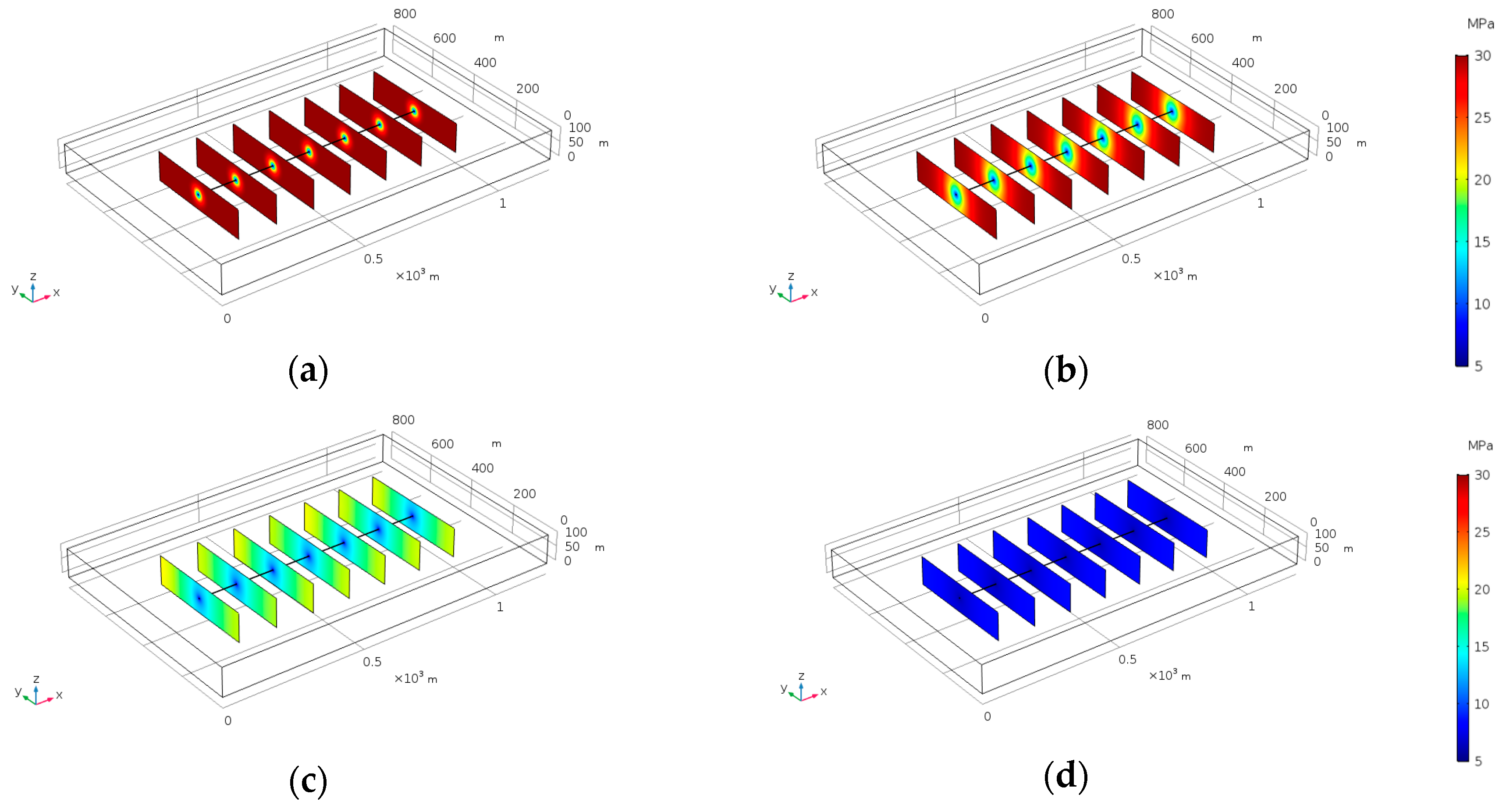
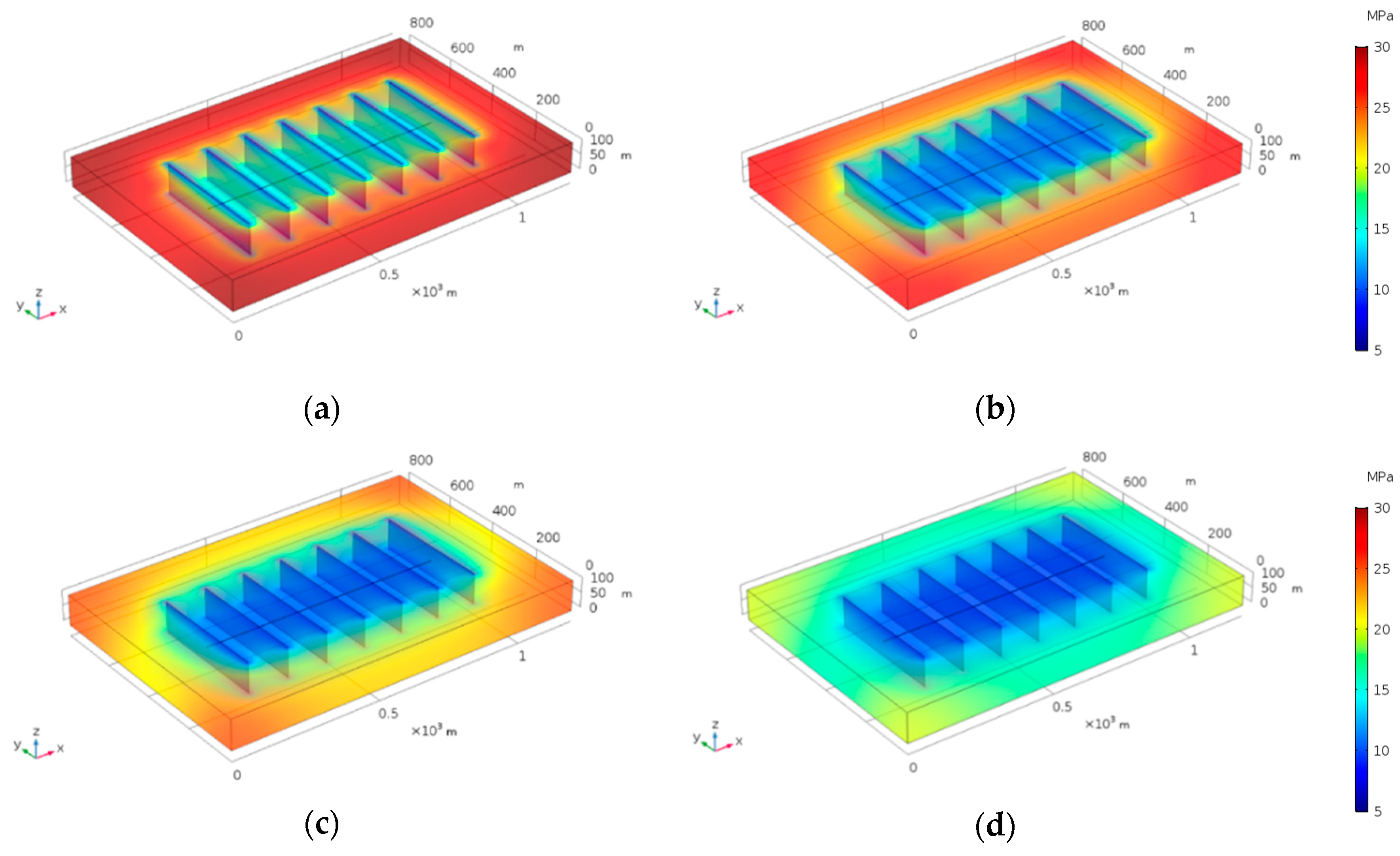
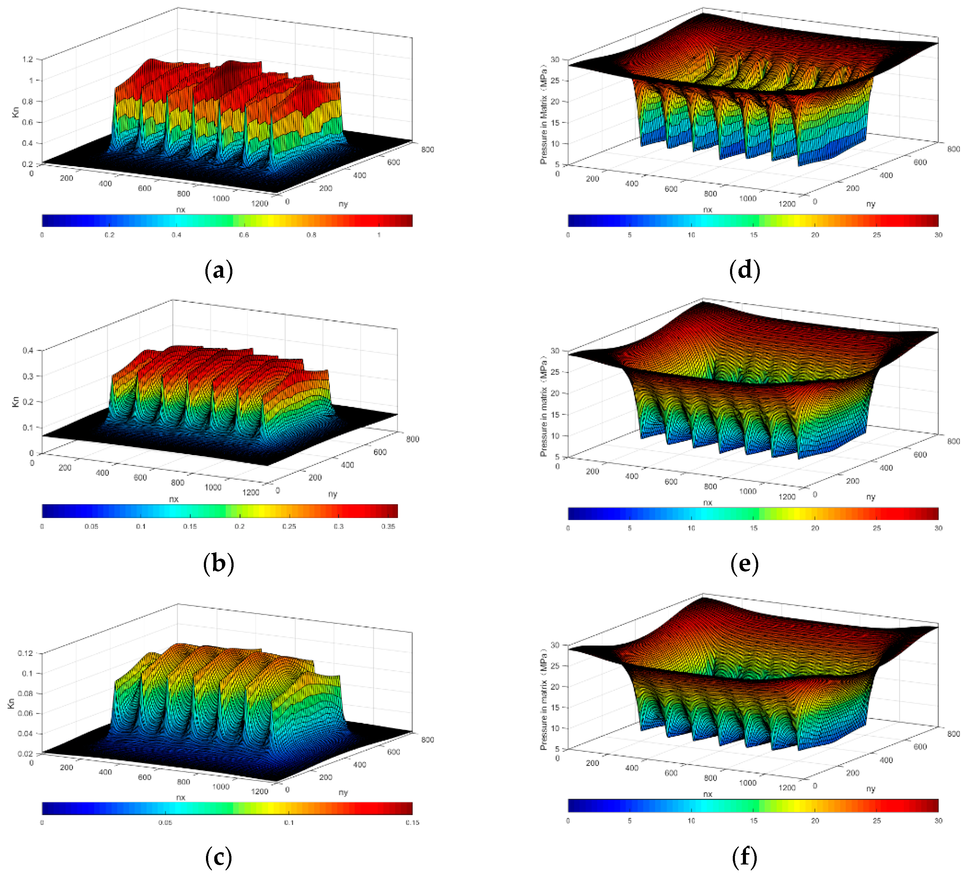
4.2.1. Pressure Distribution in Artificial Fractures

Figure 7 shows the pressure distribution in the artificial fractures at the beginning of production. The pressure distribution in the artificial fractures is related to parameters such as fracture aperture and permeability. As can be seen from the figure, due to the high conductivity of the artificial fractures, the pressure in the fracture rapidly decreases. A drawdown pressure is created between the artificial fractures and the matrix–micro-fracture system, so that gas flows from the matrix–micro-fracture system into artificial fractures and gas is produced by production well.

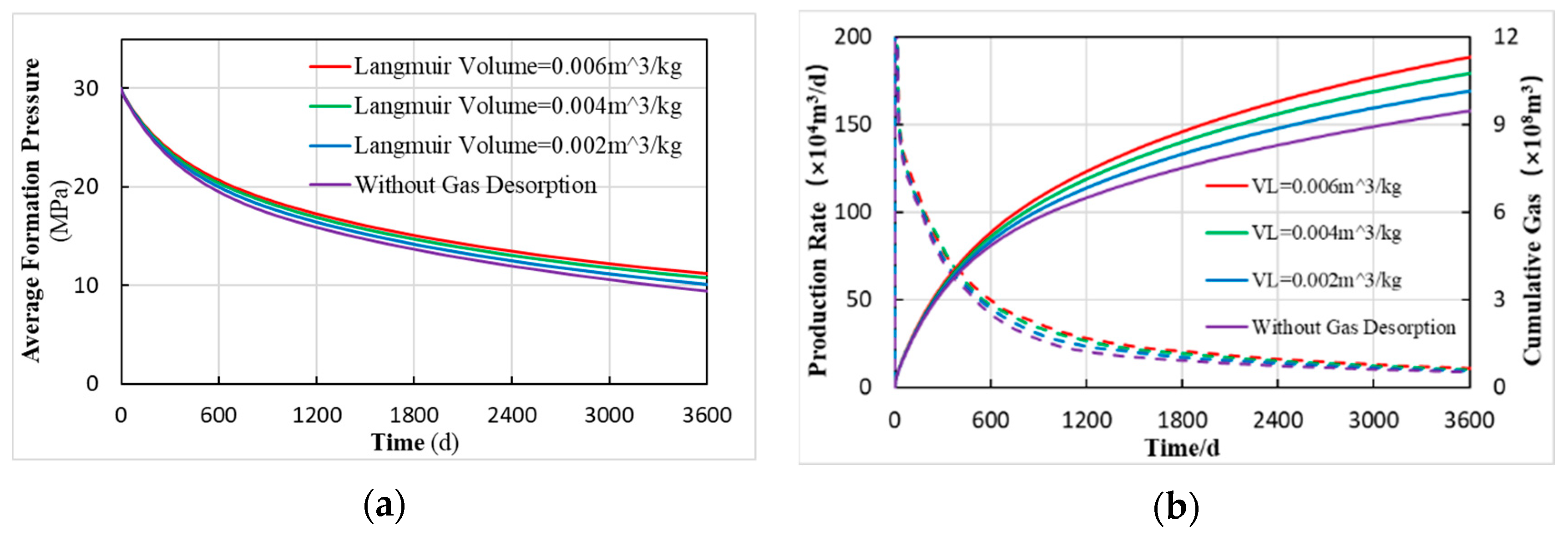
4.2.2. Gas Desorption Process

Based on the physical model parameters, the production of shale gas multi-section fractured horizontal wells is simulated. It has been shown in Figure 8 that during the first three years of production, the decline of pressure in the reservoir is mainly concentrated in the area that is near the wellbore and the hydraulic fracture faces, while the pressure drop in the outer area is very small. It shows that the produced gas mainly comes from free gas and desorption gas in the stimulated volume.

Figure 9 shows the average reservoir pressure, gas production rate, and cumulative gas production at different Langmuir volumes. We found that the desorption process has the effect of supplementing the reservoir pressure, but the effect is not significant. Since the gas production rate is affected not only by the physical properties of the reservoir, but also by the pressure distribution, the gas desorption process has limited supplementary effects on pressure, and the impact on the gas production rate is not significant. At the same time, as the Langmuir volume increases, the cumulative gas production gradually increases.

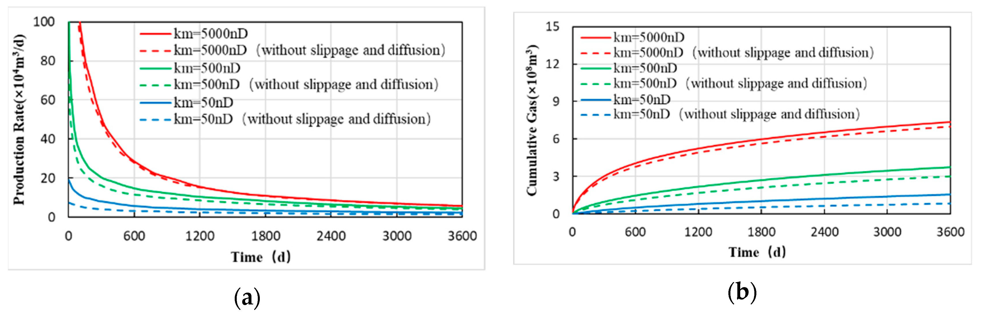
4.2.3. The Klinkenberg effect and Diffusive Gas Transport

Figure 10a–c show the Knudsen number distribution of shale gas reservoirs in fractured horizontal wells at the same time of production, under different shale matrix permeabilities. As can be seen from the figure, the closer to the artificial fractures, the larger the Knudsen number. This is due to the negative correlation between Knudsen number and pressure, so the lower the pressure, the larger the Knudsen number. At the same time, when the shale permeability decreases, the pressure drop of the artificial fractures becomes larger and the pressure drop funnel becomes steeper. Therefore, the closer the pressure gets to artificial fractures, the greater the increase of the Knudsen number.

Figure 10d–f show the matrix pressure distribution of shale gas reservoirs in fractured horizontal wells at the same time of production, under different shale matrix permeabilities. It can be seen from the figure that the pressure of the artificial fractures falls fastest, and the closer to artificial fractures, the lower reservoir pressure. Comparing the reservoir pressures under different shale permeability conditions, the lower the shale permeability, the faster the pressure of the artificial fractures drops and the fewer reservoirs are used, resulting in steeper pressure drop funnels. This is because for shale reservoirs with low permeability, it is difficult for gas to flow in such dense porous media, so the gas stored in the shale cannot be added to the artificial fractures in time when the gas in the fracturing fractures. When the gas in the artificial fractures is recovered, the pressure in the fracture rapidly decreases. Compared to shales containing nano-micro pores, gases stored in the fractures and the region near fractures are more likely to be produced to make the pressure drop faster.

Figure 11 shows the curve of the gas production rate and cumulative gas production for multi-section fractured horizontal wells with different shale permeability. As can be seen from the figure, the gas production rate and cumulative gas production increase with the increase of shale permeability, and the growth rate also increases. However, compared with the production rate and cumulative production (without considering diffusion and slippage effects), the increment of gas production rate and cumulative production (considering the diffusion and slippage effects), decreases with increasing shale permeability. This shows that when shale permeability becomes smaller (pore size decreases), Knudsen diffusion and slippage effects have a greater impact on the daily gas production and the cumulative production of fracturing horizontal wells.

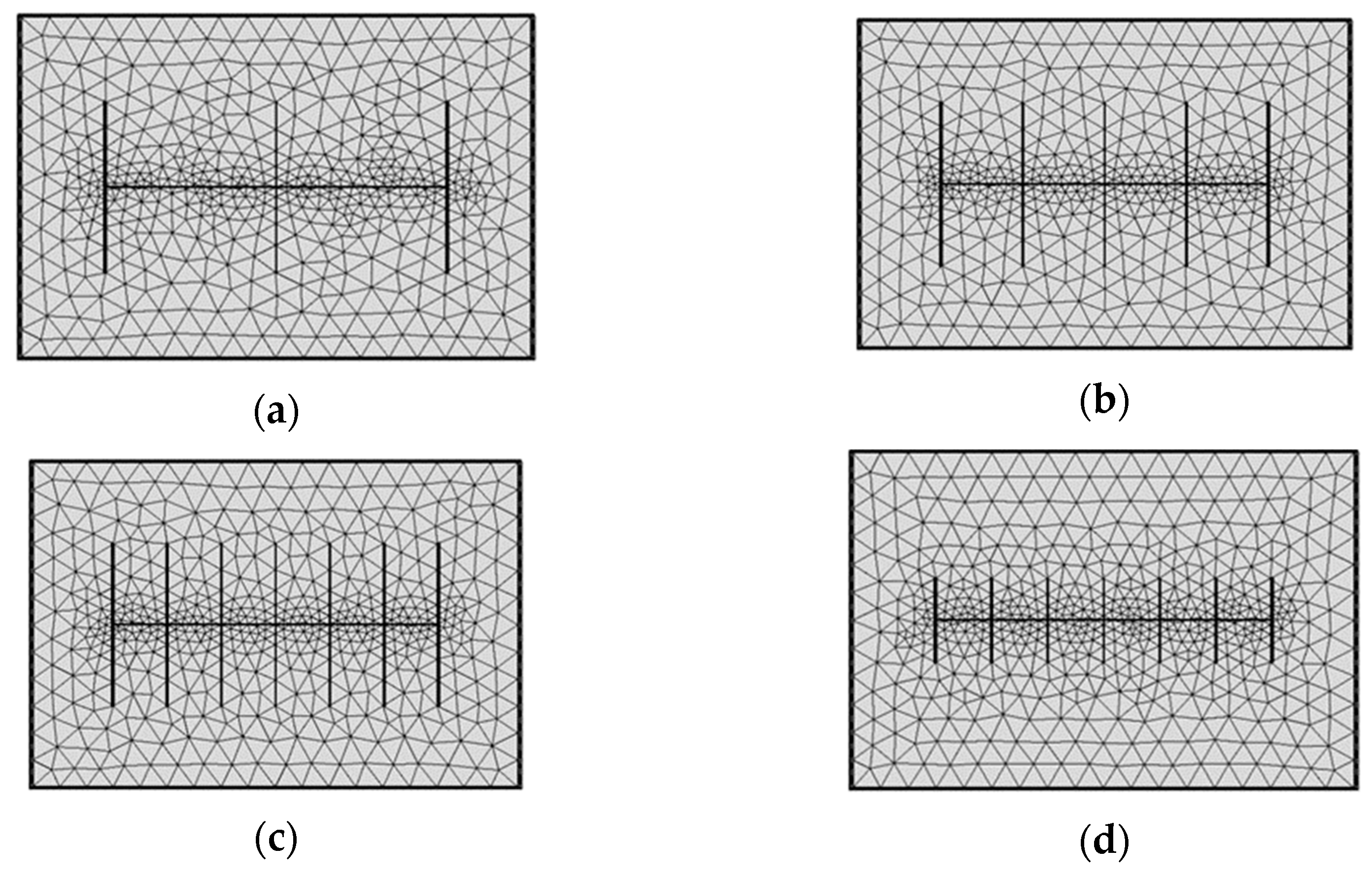
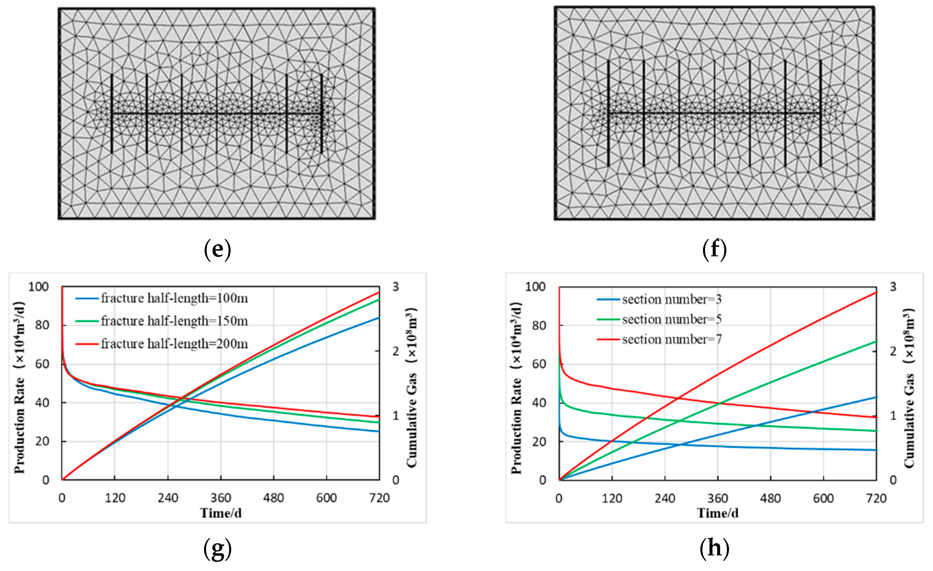
4.2.4. Artificial Fracture Morphology

Based on the above numerical model, we change the number of fractured sections (Figure 12a–c) and the half-length of artificial fractures (Figure 12d–f) to simulate the production of shale gas. It can be seen from Figure 12g that as the half-length of artificial fractures increases, the gas production rate and cumulative gas production also increase. However, the increasing rate in the gas production rate and cumulative gas production has gradually decreased. The main reason for this is that as the half-length of the artificial fractures increases, the multi-fracture interference becomes severer. Therefore, as the half-length of artificial fractures increases, the increasing rate in the gas production rate and cumulative gas production decreases.

From Figure 12h, it can be seen that the number of sections has an important influence on the gas production rate and cumulative gas production. With the increase in the section number, the gas production rate and cumulative gas production also increase. It is worth noting that as the section number increases, the rate of decline in gas production rate also increases. Similar to the previous situation, the main reason is that with the increase of the section number, the multi-fracture interference becomes severer. As a result, the larger section number, the faster the gas production rate declines.

Through analysis, it is found that excessive half-length of fractures and section numbers will generate strong multi-fracture interference, which will have a negative impact on the productivity of horizontal wells. Therefore, for a horizontal well fracturing design, the half-length of fractures and section number should not be pursued blindly, but the parameters of horizontal wells should be optimized to reduce the multi-fracture interference.

5. Conclusions

In this paper, based on the matrix–micro-fracture continuous dual model and discrete fracture model, a mathematical model of the shale gas reservoir considering a multi-scale flow mechanisms is established.

The numerical calculation format using a cell-centered variable arrangement of shale gas three-dimensional flow based on the finite volume element method is deduced. In this case, the variables and their associated quantities are stored in the centroids of the control elements. Thus, the elements are the same as the discretization elements; in general, the method is second-order accurate, because all quantities are calculated at the element and face centroids. Talyor series expansion can be used to reconstruct the variations within the cell. Another advantage of the cell-centered formulation is that it allows the use of general polygonal elements without the need for pre-defined shape functions. This permits a straightforward implementation of a full multigrid strategy.

The artificial fracture is expressed by the two-dimensional surface, and the wellbore is expressed by a one-dimensional solid based on the dimension reduction method. The finite volume element method is used to solve the multi-section fractured horizontal well productivity and pressure distribution.

Through the analysis of the simulation results, it is found that the model can reflect the initial production of shale gas and its characteristics of rapid decline. The analysis shows that the gas desorption of shale gas has a great impact on reserves, which in turn have a supplementary effect on the reservoir pressure. On one hand, with the prolongation of production time, the proportion of desorption is increased. On the other hand, shale gas production is mainly affected by the scope of stimulated volume.

According to the development process of shale gas reservoirs, a numerical model of a stimulated reservoir volume fractured horizontal well is established. The analysis shows that the pressure will rapidly decrease in artificial fractures. The desorption process has a great influence on the geological reserves, but has a limited impact on the productivity of horizontal wells. With the decrease of the pore size of the matrix, the Klinkenberg effect and gas diffusion have a greater impact on shale gas productivity. When the matrix permeability is greater than 0.01 mD, those flow mechanisms has no significant effect on the productivity. Compared with the fracture half-length, the section number has a greater impact on the productivity of shale gas. However, the excessive half-length of the fracture and the section number all induce multi-fracture interference. Therefore, the horizontal well parameters need to be optimized.

The parameters of the artificial fracture network can be conveniently adjusted and the factors affecting the productivity can be analyzed. The research content of this paper has certain theoretical and practical significance for the volume fractured design of shale gas reservoirs and the reasonable evaluation of production capacity.

References

1. Kucuk, F.; Sawyer, W.K. Transient Flow in Naturally Fractured Reservoirs and Its Application to Devonian Gas Shales. In Proceedings of the SPE Annual Technical Conference and Exhibition, Dallas, TX, USA, 21–24 September 1980. [Google Scholar]
2. Bumb, A.C.; McKee, C.R. Gas-well testing in the presence of desorption for coalbed methane and devonian shale. SPE Form. Eval. 1988, 3, 179–185. [Google Scholar] [CrossRef]
3. Carlson, E.S.; Mercer, J.C. Devonian Shale Gas Production: Mechanisms and Simple Models. J. Pet. Technol. 1991, 43, 476–482. [Google Scholar] [CrossRef]
4. Swami, V. Shale Gas Reservoir Modeling: From Nanopores to Laboratory. In Proceedings of the SPE Annual Technical Conference and Exhibition, San Antonio, TX, USA, 8–10 October 2012. [Google Scholar]
5. Saputelli, L.; Lopez, C.; Chacon, A.; Soliman, M. Design Optimization of Horizontal Wells with Multiple Hydraulic Fractures in the Bakken Shale. In Proceedings of the SPE/EAGE European Unconventional Resources Conference and Exhibition, Vienna, Austria, 25–27 February 2014. [Google Scholar]
6. Rubin, B. Accurate Simulation of Non Darcy Flow in Stimulated Fractured Shale Reservoirs. In Proceedings of the SPE Western regional meeting, Anaheim, CA, USA, 27–29 May 2010. [Google Scholar]
7. Klimkowski, Ł.; Nagy, S. Key factors in shale gas modeling and simulation. Arch. Min. Sci. 2014, 59. [Google Scholar] [CrossRef]
8. Mirzaei, M.; Cipolla, C.L. A Workflow for Modeling and Simulation of Hydraulic Fractures in Unconventional Gas Reservoirs. Geol. Acta 2012, 10, 283–294. [Google Scholar]
9. Yao, J.; Wang, Z.; Zhang, Y.; Huang, Z.Q. Numerical simulation method of discrete fracture network for naturally fractured reservoirs. Acta Pet. Sin. 2010, 31, 284–288. [Google Scholar]
10. Hoteit, H.; Firoozabadi, A. Compositional Modeling of Fractured Reservoirs without Transfer Functions by the Discontinuous Galerkin and Mixed Methods. SPE J. 2004, 11, 341–352. [Google Scholar] [CrossRef]
11. Moinfar, A.; Narr, W.; Hui, M.H.; Mallison, B.T.; Lee, S.H. Comparison of Discrete-Fracture and Dual-Permeability Models for Multiphase Flow in Naturally Fractured Reservoirs. In Proceedings of the SPE Reservoir Simulation Symposium, The Woodlands, TX, USA, 21–23 February 2011. [Google Scholar]
12. Kuuskraa, V.A.; Wicks, D.E.; Thurber, J.L. Geologic and Reservoir Mechanisms Controlling Gas Recovery from the Antrim Shale. In Proceedings of the SPE Annual Technical Conference and Exhibition, Washington, DC, USA, 4–7 October 1992. [Google Scholar]
13. Schepers, K.C.; Gonzalez, R.J.; Koperna, G.J.; Oudinot, A.Y. Reservoir Modeling in Support of Shale Gas Exploration. In Proceedings of the Latin American and Caribbean Petroleum Engineering Conference, Cartagena de Indias, Colombia, 31 May–3 June 2009. [Google Scholar]
14. Dehghanpour, H.; Shirdel, M. A Triple Porosity Model for Shale Gas Reservoirs. In Proceedings of the Canadian Unconventional Resources Conference, Calgary, AB, Canada, 15–17 November 2011. [Google Scholar]
15. Wu, Y.S.; Moridis, G.; Bai, B.; Zhang, K. A Multi-Continuum Model for Gas Production in Tight Fractured Reservoirs. In Proceedings of the SPE Hydraulic Fracturing Technology Conference, The Woodlands, TX, USA, 19–21 January 2009. [Google Scholar]
16. Aboaba, A.L.; Cheng, Y. Estimation of Fracture Properties for a Horizontal Well With Multiple Hydraulic Fractures in Gas Shale. In Proceedings of the SPE Eastern Regional Meeting, Morgantown, WV, USA, 13–15 October 2010. [Google Scholar]
17. Wang, H.T. Performance of multiple fractured horizontal wells in shale gas reservoirs with consideration of multiple mechanisms. J. Hydrol. 2014, 510, 299–312. [Google Scholar] [CrossRef]
18. Fang, W.; Jiang, H.; Li, J.; Wang, Q.; Killough, J.; Li, L.; Peng, Y.; Yang, H. A numerical simulation model for multi-scale flow in tight oil reservoirs. Pet. Explor. Dev. 2017, 44, 415–422. [Google Scholar] [CrossRef]
19. Javadpour, F. Nanopores and Apparent Permeability of Gas Flow in Mudrocks (Shales and Siltstone). J. Can. Pet. Technol. 2009, 48, 16–21. [Google Scholar] [CrossRef]
20. Ferziger, J.H.; Perić, M. Computational Methods for Fluid Dynamics. Phys. Today 1997, 50, 80–84. [Google Scholar] [CrossRef]
21. Caumon, G.; Collon-Drouaillet, P.L.C.D.; De Veslud, C.L.C.; Viseur, S.; Sausse, J. Surface-Based 3D Modeling of Geological Structures. Math. Geosci. 2009, 41, 927–945. [Google Scholar] [CrossRef] [Green Version]
22. Juanes, R.; Samper, J.; Molinero, J. A general and efficient formulation of fractures and boundary conditions in the finite element method. Int. J. Numer. Methods Eng. 2002, 54, 1751–1774. [Google Scholar] [CrossRef]
23. Çengel, Y.A.Y. Cengel, Heat and Mass Transfer: A Practical Approach, 3rd ed.; McGraw-Hill: Singapore, 2006. [Google Scholar]
24. Incropera, F.P. Fundamentals of Heat and Mass Transfer; John Wiley & Sons: Jefferson City, MO, USA, 2007. [Google Scholar]
25. Patankar, S.V. Numerical Heat Transfer and Fluid Flow; CRC Press: New York, NY, USA, 1980. [Google Scholar]
26. Darwish, M.; Moukalled, F. A new approach for building bounded skew-upwind schemes. Comput. Methods Appl. Mech. Eng. 1996, 129, 221–233. [Google Scholar] [CrossRef]
27. Spekreijse, S. Multigrid solution of monotone second-order discretizations of hyperbolic conservation laws. Math. Comput. 1987, 49, 135–155. [Google Scholar] [CrossRef]
28. Fan, D.; Yao, J.; Sun, H.; Zeng, H. Numerical simulation of multi-fractured horizontal well in shale gas reservoir considering multiple gas transport mechanisms. Chin. J. Theor. Appl. Mech. 2015, 47, 906–915. [Google Scholar]
Figure 1. Diagram of a mathematical model. (a) Multi-section fractured horizontal well grid section diagram; (b) artificial fracture diagram; (c) grid of natural micro-fractures and matrix.
Energies 11 02329 g001
Figure 2. Control cell corresponding to the different variable arrangement. (a) Cell-centered; (b) vertex-centered.
Energies 11 02329 g002
Figure 3. Gradient computation.
Energies 11 02329 g003
Figure 4. Element connectivity and face orientation using global indices.
Energies 11 02329 g004
Figure 5. Comparison of the gas production calculated using finite volume method and commercial software Eclipse.
Energies 11 02329 g005
Figure 6. A numerical model of a multi-section fractured horizontal well.
Energies 11 02329 g006
Figure 7. Pressure distribution in artificial fractures. (a) T = 0 d; (b) T = 1 d; (c) T = 2 d; (d) T = 3 d.
Energies 11 02329 g007
Figure 8. Reservoir pressure distribution at different production times. (a) T = 1a; (b) T = 3a; (c) T = 5a; (d) T = 10a.
Energies 11 02329 g008
Figure 9. Influence of gas desorption on horizontal well productivity. (a) Average reservoir pressure at different Langmuir volumes; (b) Gas production rate and cumulative gas production at different Langmuir volumes.
Energies 11 02329 g009
Figure 10. Field distribution of Knudsen number and matrix pressure in shale gas reservoir. (a) km = 10−5 mD, Kn; (b) km = 10−4 mD, Kn; (c) km = 10−3 mD, Kn; (d) km = 10−5 mD, pm; (e) km = 10−4 mD, pm; (f) km = 10−3 mD, pm.
Energies 11 02329 g010
Figure 11. The effect of Knudsen diffusion and the Klinkenberg effect on productivity. (a) Production rate at different matrix permeability; (b) Cumulative gas at different matrix permeability.
Energies 11 02329 g011
Figure 12. The effect of horizontal well parameters on productivity. (a) section number = 3; (b) section number = 5; (c) section number = 7; (d) fracture half-length = 100 m; (e) fracture half-length = 150 m; (f) fracture half-length = 200 m; (g) Three fractured sections, T = 5a; (h) Four fractured sections, T = 5a.
Energies 11 02329 g012aEnergies 11 02329 g012b