An Equivalent Circuit for the Evaluation of Cross-Country Fault Currents in Medium Voltage (MV) Distribution Networks

Abstract

A Cross-Country Fault (CCF) is the simultaneous occurrence of a couple of Line-to-Ground Faults (LGFs), affecting different phases of same feeder or of two distinct ones, at different fault locations. CCFs are not uncommon in medium voltage (MV) public distribution networks operated with ungrounded or high-impedance neutral: despite the relatively small value of LGF current that is typical of such networks, CCF currents can be comparable to those that are found in Phase-To-Phase Faults, if the affected feeder(s) consists of cables. This occurs because the faulted cables’ sheaths/screens provide a continuous, relatively low-impedance metallic return path to the fault currents. An accurate evaluation is in order, since the resulting current magnitudes can overheat sheaths/screens, endangering cable joints and other plastic sheaths. Such evaluation, however, requires the modeling of the whole MV network in the phase domain, simulating cable screens and their connections to the primary and secondary substation earth electrodes by suitable computer programs, such as ATP (which is the acronym for alternative transient program) or EMTP (the acronym for electromagnetic transient program), with substantial input data being involved. This paper presents a simplified yet accurate circuit model of the faulted MV network, taking into account the CCF currents’ return path (cable sheaths/screens, ground conductors, and earthing resistances of secondary substations). The proposed CCF model can be implemented in a general-purpose simulation program, and it yields accurate fault currents estimates: for a 20 kV network case study, the comparison with accurate ATP simulations evidences mismatches mostly smaller than 2%, and never exceeding 5%.

1. Introduction

Double line-to-ground faults, i.e., the simultaneous presence of two line-to-ground faults (LGFs) affecting different phases of a feeder or of two different lines of a given network at different locations, are often called “Cross-Country” faults (CCFs). The phenomenon is significant in MV distribution networks, which have a much higher fault rate than HV (high voltage) and EHV (extra high voltage) networks. MV networks operated with high-impedance grounded, ungrounded, or resonant neutral are particularly affected by CCFs, because a LGF causes significant overvoltages on the healthy phases, which in turn can cause a further LGF, thus resulting in a CCF. This is a not uncommon occurrence, as the temporary overvoltages can be substantial: if the network neutral is grounded by means of Petersen coil, also equipped with a parallel high resistance, the Earth-Fault-Factor (EFF) is 1.73 p.u., whereas in networks with ungrounded neutral EFF can attain 2.5–3.5 p.u. [1]. In both cases, the associated switching overvoltages are in the 2.7–4.5 p.u. range. A second fault, occurring at any weak point in the insulation (cable joint, old bushings, polluted insulators) can thus result in the CCF. The CCFs may occur both in two phases of the same feeder and in two different feeders, as described in Figure 1.

It should be pointed out that the correct selection of CCFs in MV networks operated with non-solidly grounded neutral is not always straightforward, especially in case of non-radial network topologies (e.g., closed loop) [2,3]. CCFs occur much less frequently in HV and EHV networks and they may affect the performance of distance relaying schemes; however, there are some research papers addressed in the identification and elimination of CCFs in HV and EHV networks [4,5,6,7,8,9,10,11]. Focusing now on MV networks, an important point is that, regardless of the affected network’s neutral grounding, the CCF can involve fault currents of the same order of magnitude of phase-to-phase faults: an accurate evaluation is thus required, in order to assess the chance of damage to cable screens/sheaths and joints, as well as the ground potential rise (GPR) of the involved earthing system. Under this regard, two different CCF configurations can be considered: if a CCF involves one or in two overhead lines, then the fault currents are strongly limited by the line pole earth resistances (R_p1 and R_p2 in Figure 1), which generally are in the range of some tens (even up to one hundred) Ohms. On the other hand, if both faults affect cables, currents can attain large values as anticipated, and moreover their assessment is not immediate because the fault circuit is very complex, involving not only the earth systems of the secondary and primary substations (SS and PS, respectively), but also, and mainly, the metallic cable screens (which are often connected to SS and PS ground electrodes, as shown in Figure 1).

The symmetrical components (0, 1, 2) method can be used to calculate CCF currents [12,13]. In [2], a simple equivalent circuit and formulas are proposed to evaluate CCFs occurring in overhead lines of an MV distribution network. In [14], a comparison between the symmetrical components method presented in [12] and the three-phase network solution is reported while considering low voltage distribution networks and showing a full agreement between the two solutions. However, in case of cable faults the correct evaluation of the CCF currents and their distribution between earth systems and cable screens of the faulty and healthy lines requires power system simulation softwares (e.g., alternative transient program (ATP), electromagnetic transient program (EMTP), DigSilent, etc.) modeling each system component in the phase domain, with all line conductor phases, cable screens/armours, shield/earth wires of overhead lines, counterpoise conductors: each cable/overhead-line segment is then simulated by its multiconductor nominal-pi circuit. This approach obviously allows simulating the MV distribution mixed cable-overhead networks with high accuracy, but requires in turn a very large amount of input data. Without drastic simplifications, as in [15,16,17], where CCF currents are not calculated but are considered known, manual calculations are not practical in the phase domain [18,19,20,21].

In this paper, a simple model in the phase domain is proposed in order to calculate fault currents and GPRs due to CCFs in mixed cable/overhead MV distribution network. Differently from the models that are presented in [12,13,14] and [15,16,17,18,19,20,21], the proposed lumped-circuit model does not require a full network solution with a dedicated power system simulation software, and in principle could be solved manually. The model is also capable to evaluate, with satisfying accuracy, the current distribution in the cable screens at the fault locations and at the PS. The models of the current return paths (earth and ungrounded conductors) are derived from the ones that are proposed in [22]. The model can be adapted to the study of a CCF affecting the same feeder or two different ones.

Section 2 presents the equivalent circuit of a cable line stretch with its ground current return path (screens/sheaths, solidly connected to the earthing resistances of SSs along the stretch). Section 3 describes the proposed network models for CCF calculation, when faults affect either the same or two different feeders. Finally, Section 4 shows an application of the proposed method to an MV (20 kV–50 Hz) distribution network and the validation of results by means of ATP-EMTP.

2. Equivalent Circuit of Phase-Conductors, Screens and Earth Resistances of SSs of a Cable Line Stretch

The key issue in the proposed approach is the individuation and modeling of the CCF current return paths. This amounts to building equivalent lumped circuits of Figure 2 for each stretch of the cable line of length ‘a’ with phase conductors, screens, and earth resistance of SSs [22]. Following [22], the main simplifying assumption underlying the circuits in Figure 2 is the replacement of lumped SSs earthing resistances with a uniformly distributed shunt conductance to ground. Moreover, all asymmetries, both in series impedances and in shunt capacitances, were disregarded using the relevant average values.

In Figure 2, symbols mean:

• Z_R, Z_S and Z_T are the overall self impedances of phase conductors;
• Z_sc and Y_E are the equivalent series impedance and shunt admittance of the system formed by the three screens of the cables and the earth resistance of the SSs;
• e_iR, e_iS, e_iT are the induced electromotive forces (emfs) in each phase conductor by the currents flowing both throughout the other phases and the screen conductors; and,
• e_sc is the electromotive force induced in the screens by the phase currents.

The above emfs, impedances and admittances are evaluated by the following expressions:

$$\{\begin{array}{l}{Z}_o=\sqrt{z_{sc}/y_e};k=\sqrt{z_{sc}{y}_e};z_{sc}=(z_{ss}+2z_{ms})/3;y_e=1/(R_{tss}{d}_{ss})\\ Z_{sc}=Z_o\sinh (ka);Y_E=[\cosh (ka)-1]/Z_{sc}\\ A_1=\left(z_{mps}/k\right)\sinh (ka)\\ A_2=\left(z_{mps}/z_{sc}\right)\cdot [\cosh (ka)-1];A_3=\left[z_{mpc}^2/(k{z}_{sc})\right]\cdot \left[\sinh (ka)-ka\right]\\ e_{iR}=z_{mp}a(I_S+I_T)+A_3(I_R+I_S+I_T)+A_1{I}_{sc}-A_2{E}_{sc}\\ e_{iS}=z_{mp}a(I_R+I_T)+A_3(I_R+I_S+I_T)+A_1{I}_{sc}-A_2{E}_{sc}\\ e_{iT}=z_{mp}a(I_R+I_S)+A_3(I_R+I_S+I_T)+A_1{I}_{sc}-A_2{E}_{sc}\\ e_{sc}=A_1(I_R+I_S+I_T)\end{array}$$

(1)

where:

• z_sc is the series self-impedance per unit length of the cable line screens;
• z_ss is the series self-impedance per unit length of each cable screen;
• z_ms is the mutual impedance per unit length between the screens;
• y_e the shunt earth conductance per unit length of the SSs;
• Z_o and k are the surge impedance and the propagation constant of the uniformly distributed system formed by cable screens and earth admittance of SSs; and,
• z_mpc is the mutual impedance per unit length between phase conductors and cable screens.

For each of the above impedances and admittances per unit length, average values have been considered. In particular, the earth resistances of the SSs are considered to be uniformly distributed, while taking into account a conductance per unit length equal to:

$$g_{ESS}=\frac{1}{R_{ESS}{d}_{SS}},$$

where R_ESS is the SS earth resistance and d_SS is the distance between two adjacent SSs (both assumed equal to average values). To take into account of each actual cable line between two SSs and of each earth resistance of SSs, the equivalent circuit of Figure 2a can be replaced by the one of Figure 2b, where the constants Z_R, Z_S, Z_T, Z_sc, Y_E, e_iR, e_iS, e_iT, e_Scs, and e_Scd can be evaluated, as reported in [23].

3. Equivalent Circuits of MV Distribution Network During CCFs

3.1. CCF Occurring in the Two Different MV Feeders

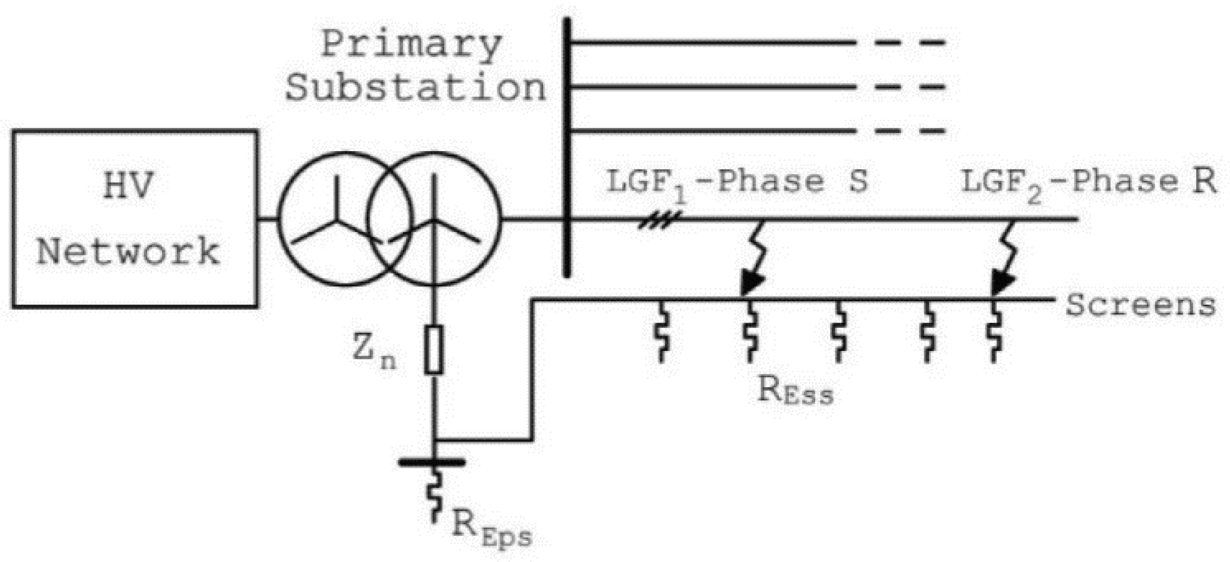
Figure 3 shows the single-line diagram of a radial MV distribution network when a CCF involves two different MV cable lines.

Figure 4 illustrates the equivalent circuit to be solved in order to calculate the CCF currents, the currents flowing in the cable screens and the GPR at fault locations. In this case, the mutual inductive coupling between phase conductors of faulty lines can be disregarded, because the LGFs occur in two different feeders; therefore, only the faulty phases of each line may be represented. The healthy feeders are simulated by the ground equivalent impedance Z_EHF, which takes into account cable screens and earth resistances of SSs, connected in parallel to the PS local earth, which are simulated by the resistance R_Eps. Generally, primed quantities in Figure 4 refer to the line stretch between the fault location and the line end. Quantities in Figure 4 mean:

• E_S, E_R and E_T are the voltages imposed by the HV network;
• Z_TR, Z_TS, Z_TT, are the self impedances of each phase of the HV/MV PS transformer;
• Z_mTR is the average value between phases of the mutual impedance of the transformer phases;
• Z_R, Z_S are the self-impedances of the phase R-feeder 1 and of phase S-feeder 2, both affected by LGF, from the HV/MV PS to fault locations;
• e_iR = A₃·I_R + A₁·I_sc1 − A₂·E_sc1 and E_Is = A₃·I_S + A₁·I_sc2 − A₂·E_sc2 are the emfs induced on the faulted phases (R and S) by the currents flowing through the screens from the fault location to the HV/MV PS;
• Z_sc1, Y_E1, Z_sc2, Y_E2, are the equivalent impedances and admittances, for the line stretch from PS up to LGF, of the system formed by screens and earth resistances of the SSs, calculated with (1);
• Z’_sc1, Y’_E1, Z’_sc2 and Y’_E2 are the equivalent impedances and admittances, from the fault location to the line end, of the system formed by screens and earth resistances of SSs, calculated with (1);
• e_sc1 = A₁·I_R, e_sc2 = A₁·I_S are the induced emfs in the screens of each feeder by phase currents I_R and I_S, respectively, and for each feeder A₁ is calculated as A₁ in (1), where the line length a that must be considered is the one between the fault location and the PS;
• C_oR is the overall line-to-ground network capacitance, considered as connected to the PS MV busbars;
• R_ESS1 and R_ESS2 are the earth resistances of the SSs involved by CCF; and,
• R_a1, R_a2 and R_a3 are used to simulate the screen connection to the PS local earth: for each of such resistances, 1 mΩ simulates the connection, 1 mΩ simulates the disconnection.
• Z_n in the neutral compensating impedance.

Furthermore, it is also possible to model overhead lines in turn of cable lines, simply by assigning suitable values to electrical constants of the line.

In the circuit of Figure 4, the unknown node voltages and branch currents can be easily calculated by solving the linear system obtained by simply applying the Kirchhoff’s current law to the nine nodes and the Ohm’s law to the 21 branches of the network.

3.2. CCF Occurring in the Same MV Feeder

Figure 5 shows the single-line diagram of radial MV distribution network when a CCF occurs only in one MV feeder, between phase R and S at different locations along the line.

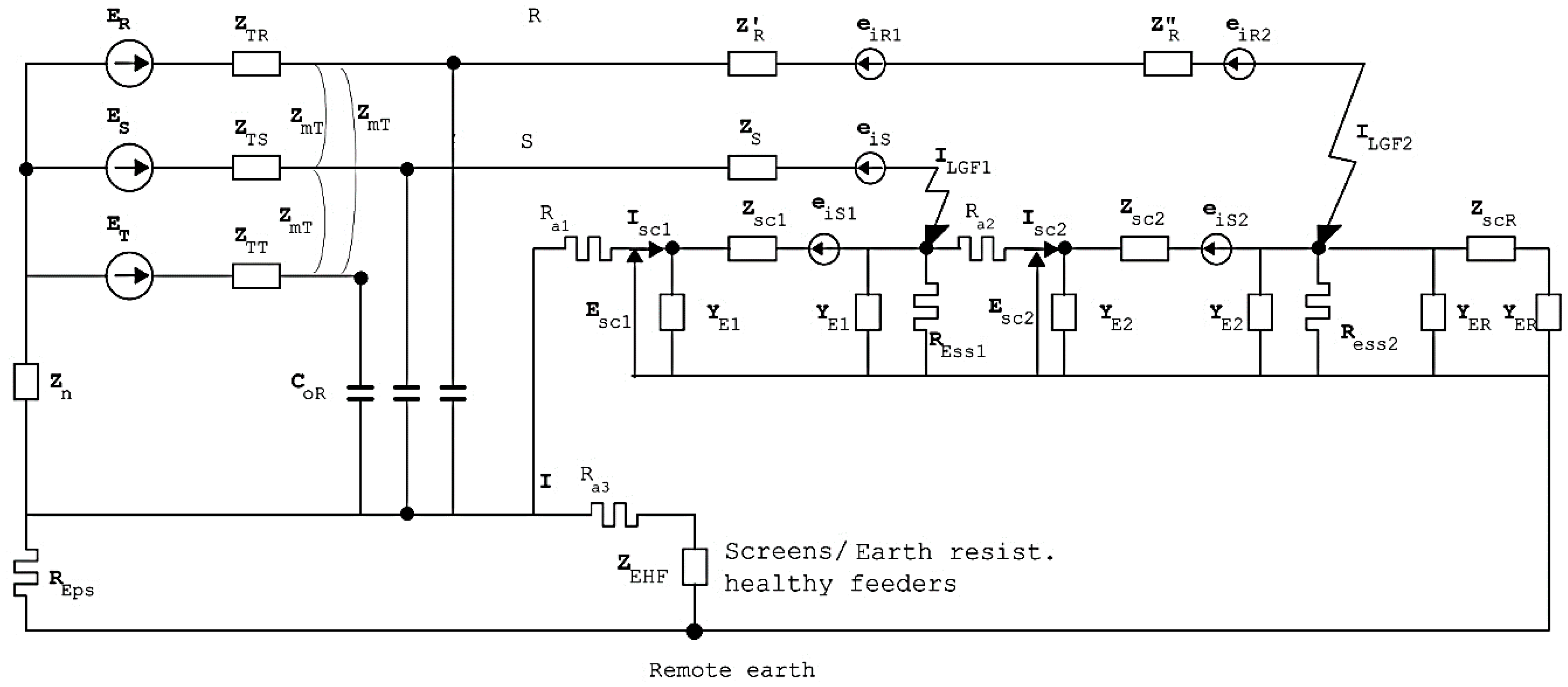
Figure 6 illustrates the equivalent circuit to be solved to calculate the CCF currents, the currents flowing in the cable screens and the GPR at fault locations.

The mutual coupling between the faulted phases (R and S in Figure 5) is taken into account only for the line stretch between the PS busbars and the closest fault (LGF1 on phase S in Figure 6). Generally, the primed quantities in Figure 6 refer to the first line stretch, between PS busbars and LGF1, whereas double-primed quantities in Figure 6 refer to the phase R stretch downstream of the LGF1 abscissa and up to LGF2. Quantities in Figure 6 are the same as those in Figure 4, except for the following ones:

• Z′_R, Z″_R are the self-impedances of the two stretches of phase R of the faulty feeder;
• Z_S is the self-impedance of the stretch of phase S up to LGF1 location of the faulty feeder;
• Z_sc1, Y_E1, Z_sc2, and Y_E2 are the equivalent impedances and admittances of the two stretches of the system composed by screens and earth resistances of the SSs of the faulty feeder;
• Z_scR and Y_ER are the equivalent impedance and admittance of the stretch, from the farther LGF to line end, of the system formed by screens and earth resistances of the SSs of the faulty feeder;
• e_iR1, e_iR2 and e_iS are the induced emfs in phase R and phase S by the currents flowing both in the screens and in phase conductors, calculated as

  $$\{\begin{array}{l}{e}_{iR1}=A_3^{\prime }(I_R+I_S)+A_1^{\prime }{I}_{sc1}-A_2^{\prime }{E}_{sc1}+Z_{mc}{a}_1{I}_S\\ e_{iR2}=A_3^{\prime \prime }{I}_R+A_1^{\prime \prime }{I}_{sc2}-A_2^{\prime \prime }{E}_{sc2}+Z_{mc}{a}_2{I}_R\\ e_{iS}=A_3^{\prime }{I}_S+A_1^{\prime }{I}_{sc1}-A_2^{\prime }{E}_{sc1}+Z_{mc}{a}_1{I}_R\end{array}$$

  (2)
• e_iS1 = A′₁·(I_R + I_S), e_iS2 = A″₁·I_R are the emfs in the screens of the feeder induced by phase currents; and,
• R_a2 allows for considering connection (R_a2 = 1 mΩ) or disconnection (R_a2 = 1 mΩ) at fault location between the screens of the first and second line stretch.

Furthermore, as in the previous case, it is also possible to model overhead lines in turn of cable lines, simply by assigning suitable values to electrical constants of the line.

The behaviour of the circuit of Figure 6 can be easily calculated by solving the linear system obtained by applying the Kirchhoff’s current law to the eight nodes and the Ohm’s law to the 18 branches of the network.

3.3. Summary of the Proposed Methodology

The proposed methodology can be summarized as follows:

(1)

Network data acquisition

a.

Transformer nameplate data, winding connection;

b.

Neutral grounding status (if necessary, grounding impedance data);

c.

Faulted line(s) data (positive sequence impedances, zero sequence capacitances); and,

d.

Return path data (cable sheath impedances and capacitances, sheath/substation earthing resistances, overhead line ground wire, if any, impedances and tower earthing resistances).

(2)

Selection of ground faults (LGF1 and LGF2)

(3)

Synthesis of the return path circuit(s) [the actual extent depends on fault location, i.e., item 2; the following steps refer to a single stretch of the return path]

e.

Spatial averaging of the sheath / secondary substation / tower earthing resistances to obtain the equivalent distributed grounding admittance Y_E

f.

Calculation of the distributed circuit parameters for the return path and of the equivalent source e_s

(4)

Overall fault network assembly (depending on the faults’ locations the equivalent circuit of Figure 4 or Figure 6 is arrived at)

(5)

Solve the fault network

4. Comparison between the Proposed Circuit Model and the Accurate ATP Model of a 20 kV Mixed Overhead/Cable Network

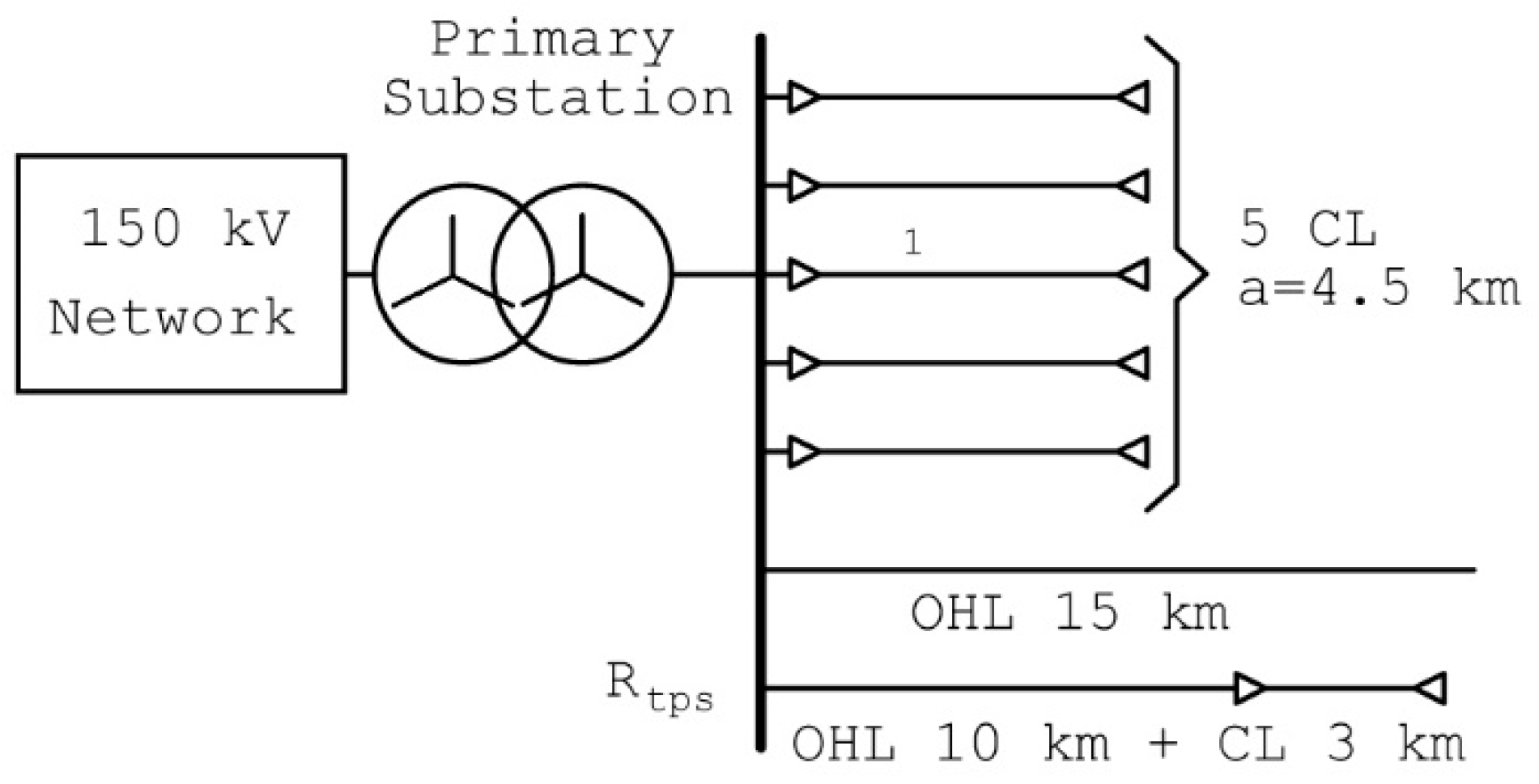
In order to verify the accuracy of the proposed CCF-models, a comparison study is carried out in this section for the 20 kV–50 Hz distribution network that is depicted in Figure 7.

The network is made up of:

• five cable lines (CLs) each 4.5 km long equipped with 185 mm²-Al conductors 16 mm²-Cu screens; all distances between SSs are equal to 0.5 km;
• a 15 km long overhead line (OHL) equipped with 70 mm² Al conductors; and,
• a mixed overhead-cable line (ML) composed by a 10 km long OHL equipped with 70 mm² Al conductors and a 3 km long CL equipped with 185 mm²-Al conductors 16 mm²-Cu screens.

The main electrical constants of the network components are reported in

Table 1. Electrical parameters of the main components of the studied 150/20 kV–50 Hz system.

Component	Electrical Parameters
PS transformer	Rated power Nt = 40 MVA	Rated voltages Vn1/Vn2 = 150 kV/20 kV	Short circuit impedance Zsc = 0.13 p.u.
CLs	Phase self impedance 0.2028 + j0.7495 Ω/km	Phase/phase mutual impedance 0.0492 + j0.6441 Ω/km	Screen self impedance 1.053 + j0.6896 Ω/km	Screen/Screen mutual impedance 0.0492 + j0.6441 Ω/km	Phase/screen mutual impedance 0.0492 + j0.6620 Ω/km
OHL	Phase self impedance 0.4783 + j 0.7 Ω/km	Phase/phase mutual impedance 0.0493 + j0.35 Ω/km
Ground resistance	SSs RESS = 5–10 Ω	PS REPS = 2 Ω	OHL REPOHL = 30 Ω

. The overall line-to-ground capacitance of the studied test network is C_0R = 333 nF. The network is operated with ungrounded neutral.

4.1. CCF Occurring in Two Different Feeders of the Case Study 20 kV Network

In order to verify the accuracy of the proposed model, the test network has been simulated by means of an ATP accurate model; the results of the ATP accurate model have been thus compared to results that were obtained by the proposed simplified model. The following cases of CCF have been analysed:

(a)

LGF1in CL1, 1 km far from the PS; LGF2 at the end of the 2nd CL; the value of the SS earth resistances is R_ESS = 5 Ω;

(b)

LGF1 in CL1, 1 km far from the PS; LGF2 in CL2, 1 km far from the PS; the value of the SS earth resistances is R_ESS = 5 Ω;

(c)

LGF1 in OHL1, 10 km far from the PS; LGF2 in OHL2, 5 km far from the PS; the value of the SS earth resistances is R_ESS = 10 Ω and the one of the line poles is R_EPOHL = 30 Ω;

(d)

LGF1 in OHL, 10 km far from the PS; LGF2 in CL, 3 km far from the PS; the value of the SS earth resistances R_ESS = 10 Ω and the one of the line pole is R_EPOHL = 30 Ω; and,

(e)

LGF1 in CL1, 3 km far from the PS; LGF2 in CL2, 1 km far from the PS; the value of the SS earth resistances is R_ESS = 5 Ω.

In all cases, the cable screens are connected to PS earth, as usual practice. Only in case (e), the screens are considered to be disconnected from the earth of the PS. This countermeasure can be implemented in order to reduce the CCF currents when the LGFs occur in different feeders.

Table 2. Simulation results for CCFs occurring in two different feeders.

Case	Network Model	LG Fault Distance from PS (km)		CCF Current (kA)		Max. Screen Current at Fault Location (kA)		GPR at Fault Location (kV)		Screen Current at PS (kA)		Earth Current at PS (kA)
		LGF1	LGF2	LGF1	LGF2	LGF1	LGF2	LGF1	LGF2	Line1	Line2
(a)	Proposed	1 CL	4.5 CL	4.86	4.88	4.19	4.45	1.14	2.52	3.99	3.83	0.152
	ATP			4.85	4.84	4.18	4.40	1.19	2.65	4.06	3.81	0.153
(b)	Proposed	1 CL	3 CL	5.53	5.55	4.78	4.72	1.27	1.82	4.55	4.35	0.143
	ATP			5.54	5.53	4.77	4.67	1.33	1.84	4.64	4.35	0.142
(c)	Proposed	10 OHL	5 OHL	0.520	0.483	N/A	N/A	1.044	4.83	N/A	N/A	N/A
	ATP			0.522	0.482	N/A	N/A	1.045	4.82	N/A	N/A	N/A
(d)	Proposed	10 OHL	3 OHL	0.535	0.563	N/A	0.464	16.06	0.350	N/A	0.369	0.064
	ATP			0.535	0.563	N/A	0.455	16.06	0.351	N/A	0.357	0.071
(e) *	Proposed	3 CL	1 CL	3.76	3.74	2.55	2.12	2.29	3.05	N/A	N/A	0.007
	ATP			3.87	3.82	2.70	2.08	2.24	3.16	N/A	N/A	0.004

* Cable screens of faulty lines not connected to the PS earth.

reports the results that were obtained for the CCF currents, the maximum screen currents at fault locations, the GPR at fault locations, the screen currents of faulty lines at PS, and the current in PS earth, by both the proposed simplified approach and the ATP accurate model. The comparison between the results that were obtained by the two different models evidences that the highest errors made by the proposed simplified method is low and more than satisfactorily; in particular highest errors are:

• 2.8% for fault current;
• 2% for screen currents at fault locations;
• 3.5% for GPR at fault locations; and,
• 1.9% for screen currents at PS.

4.2. CCF Occurring in the Same Feeder of the Case Study 20 kV Network

For this CCF the following cases are analysed:

(a)

LGF1 in CL1, 1 km far from the PS; LGF2 in CL1, 4 km far from the PS; value of the SS earth resistances is R_ESS = 5 Ω;

(b)

LGF1 and LGF2 in OHL, 10 km and 15 km far from the PS, respectively; value of the pole earth resistances are R_EPOHL1 = 30 Ω and R_EPOHL2 = 15 Ω;

(c)

LGF1 in OHL, 10 km far from the PS; LGF2 in same feeder but in CL, 3 km from the end of the OHL; the value of the SS earth resistance is R_ESS = 10 Ω and the one of the line pole R_EPOHL = 30 Ω; and,

(d)

As case (f), but with cable screens disconnected from the PS earth.

Results are reported in

Table 3. Simulation results for CCFs occurring in the same 20 kV feeder.

Case	Network Model	LG Fault Distance from PS (km)		CCF Current (kA)		Max. Screen Current at Fault Location (kA)		GPR at Fault Location (kV)		Screen Current at PS (kA)
		LGF1	LGF2	LGF1	LGF2	LGF1	LGF2	LGF1	LGF2
(f)	Proposed	1 CL	4 CL	5.62	5.61	4.74	4.96	1.08	2.21	0.97
	ATP			5.59	5.58	4.74	4.91	1.14	2.15	1.01
(g)	Proposed	10 OHL	15 OHL	0.363	0.331	N/A	N/A	10.89	4.96	N/A
	ATP			0.362	0.330	N/A	N/A	10.87	4.96	N/A
(h)	Proposed	10 OHL	3 CL	0.470	0.511	N/A	0.419	14.10	0.92	N/A
	ATP			0.472	0.500	N/A	0.435	14.16	0.88	N/A
(i) *	Proposed	1 CL	4 CL	5.68	5.67	4.89	5.00	1.78	2.12	N/A
	ATP			5.66	5.66	4.81	4.92	1.74	2.11	N/A

* As case (f) but with cable screens disconnected from the PS earth.

.

Also, in this case, the proposed method provides values of currents and voltages of interest that are in good agreement with those obtained by means of the ATP accurate model; in particular, the highest errors are:

• 2.2% for fault current;
• 3.6% for screen currents at fault locations;
• 4.5% for GPR at fault locations; and,
• 4.0% for screen currents at PS.

Simulations were repeated for different types of neutral grounding, namely “resonant” (i.e., Petersen coil) and “compensated” (Petersen coil in parallel with a resistance) grounding, without evidencing any significant change in accuracy. Mismatches between the proposed model and the accurate ATP model depend on the simplifying assumptions that are described in Section 2 and Section 3 and briefly summarized in the following:

• Due to the distributed grounding model used for the current return path, errors tend to increase for shorter cables and/or faults closer to the PS busbars.
• The longitudinal asymmetries associated to horizontally arranged untransposed conductors are neglected (average values for the self and mutual phase impedances are used).
• Non-homogeneous feeders made of several different cable and/or overhead line stretches are replaced by a single “average” feeder model. A better accuracy could be achieved by representing such feeders with the cascade of the individual equivalent circuits of the constituent stretches. The resulting network would be, however, more complex than those that are depicted in Figure 4 and Figure 6.

Work is currently underway on a quick software tool for the above described detailed modeling of inhomogeneous feeders. For urban MV cable networks, with feeders including one or two cable types, the models presented in the paper yield results differing no more than 3–4% from the detailed ATP-EMTP detailed simulations. In case of overhead feeders, mismatches with ATP-EMTP are instead negligible.

In conclusion, it can be stated that the proposed circuits are able to evaluate with satisfactory accuracy the CCF currents and voltages of interest; furthermore, the proposed simplified model can be implemented very easily, also in a simple mathematical spreadsheet.

5. Conclusions

The paper presented a simplified circuit approach in the phase domain for the calculation of the cross-country fault currents: a key feature is the use of an equivalent circuit for the fault currents’ return path (grounded conductors, earthing systems, and ground). A complete formulation for the two cases of cross-country fault

• both ground faults occurring in the same feeder, or
• ground faults affecting two different feeders,

is given: the approach is applicable to overhead lines as well as to cables, the solution of the model is straightforward and it can be demanded to any generic purpose simulation software. Besides the calculation of cross-country fault currents, the model also allows for evaluating, with satisfying accuracy, the current distribution in cable screens, both at the fault locations and at the PS. The effectiveness of the proposed approach was verified by analyzing several case studies on an actual 20 Kv-50 Hz mixed cable/overhead public distribution network. Results were subsequently compared with those that were yielded by simulations carried out on a very detailed ATP-EMTP multiconductor model of the whole network. Mismatches between the proposed method and ATP-EMTP never exceeded 5% and were in the 1‒2% range in the vast majority of cases, also for both sheath/screen and earthing resistance currents.

Further studies are ongoing, aiming at a quicker automated set up of the return path equivalent circuit.

References

- Cerretti, A.; Gatta, F.M.; Geri, A.; Lauria, S.; Maccioni, M.; Valtorta, G. Ground fault temporary overvoltages in MV networks: evaluation and experimental tests. IEEE Trans. Power Deliv. 2012, 27, 1592–1600. [Google Scholar] [CrossRef]
- Codino, A.; Gatta, F.M.; Geri, A.; Lamedica, R.; Lauria, S.; Maccioni, M.; Ruvio, A.; Calone, R. Cross-country fault protection in Enel Distribuzione’s experimental MV loop lines. In Proceedings of the 2016 Power Systems Computation Conference (PSCC 2016), Genoa, Italy, 20–24 June 2016. [Google Scholar]
- Codino, A.; Gatta, F.M.; Geri, A.; Lauria, S.; Maccioni, M.; Calone, R. Detection of cross-country faults in medium voltage distribution ring lines. In Proceedings of the 2017 AEIT International Annual Conference (AEIT 2017), Cagliari, Italy, 20–22 September 2017. [Google Scholar]
- Swetapadma, A.; Yadav, A. All shunt fault location including cross-country and evolving faults in transmission lines without fault type classification. Electr. Power Syst. Res. 2015, 123, 1–12. [Google Scholar] [CrossRef]
- Makwana, V.H.; Bhalja, B. New adaptive digital distance relaying scheme for double infeed parallel transmission line during inter-circuit faults. IET Gener. Transm. Distrib. 2011, 5, 667–673. [Google Scholar] [CrossRef]
- Xu, Z.Y.; Li, W.; Bi, T.S.; Xu, G.; Yang, Q.X. First-zone distance relaying algorithm of parallel transmission lines for cross-country nonearthed faults. IEEE Trans. Power Deliv. 2011, 26, 2486–2494. [Google Scholar] [CrossRef]
- Hasheminejad, S.; Seifossadat, S.G.; Joorabian, M. New travelling-wave-based protection algorithm for parallel transmission lines during inter-circuit faults. IET Gener. Transm. Distrib. 2017, 11, 3984–3991. [Google Scholar] [CrossRef]
- Bi, T.; Li, W.; Xu, Z.; Yang, Q. First-zone distance relaying algorithm of parallel transmission lines for cross-country grounded faults. IEEE Trans. Power Deliv. 2012, 27, 2185–2192. [Google Scholar] [CrossRef]
- Sanaye-Pasand, M.; Jafarian, P. Adaptive protection of parallel transmission lines using combined cross-differential and impedance-based techniques. IEEE Trans. Power Deliv. 2011, 26, 1829–1840. [Google Scholar] [CrossRef]
- Sharafi, A.; Sanaye-Pasand, M.; Jafarian, P. Non-communication protection of parallel transmission lines using breakers open-switching travelling waves. IET Gener. Transm. Distrib. 2012, 6, 88–98. [Google Scholar] [CrossRef]
- Sharafi, A.; Sanaye-Pasand, M.; Jafarian, P. Ultra-high-speed protection of parallel transmission lines using current travelling waves. IET Gener. Transm. Distrib. 2011, 5, 656–666. [Google Scholar] [CrossRef]
- Clarke, E. Circuit Analysis of AC Power Systems—Volume 1; Wiley: New York, NY, USA, 1950; pp. 197–223. ISBN 933304261X. [Google Scholar]
- Wagner, C.F.; Evans, R.D. Symmetrical Components; Robert, E., Ed.; Krieger Publishing: Malabar, FL, USA, 1982; ISBN 089874556X. [Google Scholar]
- Sutherland, P.E. Double contingency ground fault current evaluation. IEEE Power Eng. Rev. 2002, 22, 59–61. [Google Scholar] [CrossRef]
- Campoccia, A.; Riva Sanseverino, E.; Zizzo, G. Double earth fault effects in presence of interconnected earth electrodes. In Proceedings of the 20th International Conference on Electricity Distribution (CIRED 2009), Prague, Czech Republic, 8–11 June 2009. [Google Scholar]
- Campoccia, A.; Zizzo, G. Results of the research on global earthing systems: A contribution to the problem of their identification. Int. Rev. Electr. Eng. 2013, 8, 411–421. [Google Scholar]
- La Cascia, D.; Zizzo, G. Effects of double ground faults in wind farms collector cables. In Proceedings of the 2015 IEEE 15th International Conference on Environment and Electrical Engineering (EEEIC 2015), Rome, Italy, 10–13 June 2015. [Google Scholar]
- Roy, L. Generalised polyphase fault-analysis program: calculation of cross-country fault. IET Digit. Libr. 1979, 126, 995–1001. [Google Scholar] [CrossRef]
- Laughton, M.A. The analysis of unbalanced polyphase networks by the method of phase co-ordinates. Part 1. System representation in phase frame of reference. IET Digit. Libr. 1968, 115, 1163–1172. [Google Scholar] [CrossRef]
- Laughton, M.A. Analysis of unbalanced polyphase networks by the method of phase co-ordinates. Part 2. Fault analysis. IET Digit. Libr. 1969, 116, 857–865. [Google Scholar] [CrossRef]
- Zhang, X.; Soudi, F.; Shirmohammadi, D.; Cheng, C.S. A distribution short circuit analysis approach using hybrid compensation method. IEEE Trans. Power Syst. 1995, 10, 2052–2059. [Google Scholar] [CrossRef]
- Gatta, F.M.; Iliceto, F. Calculation of current flow in grounding systems of substations and of HV line towers in line shield wires and cable sheaths during earth faults. Eur. Trans. Electr. Power 1998, 8, 81–90. [Google Scholar] [CrossRef]
- Gatta, F.M.; Iliceto, F.; Lauria, S. Nuove formule di calcolo dell’impedenza omopolare delle linee elettriche aeree di AT. L’Energia Elettrica–Ricerche 2002, 79. [Google Scholar]
Figure 1.
Medium voltage (MV) public distribution network with Cross-Country faults (CCFs) in different lines and locations.
Figure 2.
Equivalent circuit of a cable line stretch of length ‘a’ with phase conductors, screens, and earth resistance of secondary substation (SS).
Figure 3.
Single line diagram of a MV distribution network with CCF occurring in different cable lines.
Figure 4.
Equivalent circuit of a MV distribution network in case of a CCF occurring in two different cable lines.
Figure 5.
Single line diagram of a MV distribution network with CCF in the same cable line.
Figure 6.
Equivalent circuit of a MV distribution network in case of a CCF occurring in the same cable line.
Figure 7.
Single line diagram of the studied 20 kV–50 Hz distribution network.