One-Log Call Iterative Solution of the Colebrook Equation for Flow Friction Based on Padé Polynomials

Abstract

The 80 year-old empirical Colebrook function $\xi$, widely used as an informal standard for hydraulic resistance, relates implicitly the unknown flow friction factor $\lambda$, with the known Reynolds number $Re$ and the known relative roughness of a pipe inner surface ${\epsilon }^{*}$; $\lambda =\xi \left(Re,{\epsilon }^{*},\lambda \right)$. It is based on logarithmic law in the form that captures the unknown flow friction factor $\lambda$ in a way that it cannot be extracted analytically. As an alternative to the explicit approximations or to the iterative procedures that require at least a few evaluations of computationally expensive logarithmic function or non-integer powers, this paper offers an accurate and computationally cheap iterative algorithm based on Padé polynomials with only one $log$-call in total for the whole procedure (expensive $log$-calls are substituted with Padé polynomials in each iteration with the exception of the first). The proposed modification is computationally less demanding compared with the standard approaches of engineering practice, but does not influence the accuracy or the number of iterations required to reach the final balanced solution.

1. Introduction

The empirical Colebrook equation [1,2] implicitly relates the unknown flow friction factor $\lambda$ with the known Reynolds number $Re$ and the know relative roughness of inner pipe surface, ${\epsilon }^{*}$; $\lambda =\xi \left(Re,{\epsilon }^{*},\lambda \right)$, where $\xi$ is functional symbol, Equation (1).

$$\frac{1}{\sqrt{\lambda }}=-2·{\mathit{log}}_{10}\left(\frac{2.51}{Re}·\frac{1}{\sqrt{\lambda }}+\frac{{\epsilon }^{*}}{3.71}\right)$$

(1)

In Equation (1) $Re$ is Reynolds number; $4000<Re<{10}^8$, ${\epsilon }^{*}$ is relative roughness of inner pipe surface; $0<{\epsilon }^{*}<0.05$, and $\lambda$ is Darcy flow friction factor; $0.0064<\lambda <0.077$ (all three quantities are dimensionless). All values are in correlation with the diagram of Moody [3,4,5].

The Colebrook equation is based on experiments performed by Colebrook and White in 1937 with the flow of air through a set of artificially roughened pipes [2]. The accuracy of this 80 year-old equation is disputed many times [6,7,8] but it is still accepted in engineering practice as an informal standard for hydraulic resistance. Therefore, to repeat results and for comparisons, it is required to solve the Colebrook equation accurately. Numerous evaluations of flow friction factor such as in the case of complex networks of pipes pose extensive burden for computers, so not only an accurate but also a simplified solution is required. Calculation of complex water or gas distribution networks [9] which requires few evaluations of logarithmic function for each pipe, presents a significant and extensive burden which available computer resources hardly can easily manage [10,11,12,13,14].

The Colebrook equation is based on logarithmic law where the unknown flow friction factor $\lambda$ is given implicitly, i.e., it appears on both sides of Equation (1) in form $\lambda =\xi \left(Re,{\epsilon }^{*},\lambda \right)$, from which it cannot be extracted analytically (an exception is through the Lambert $W$-function [15,16,17]). The common way to solve it is to guess an initial value ${\lambda }_0$ for friction factor and then to try to balance it using the iterative algorithm [18] which needs to be terminated after the certain number of iterations when the final balanced value ${\lambda }_n$ is reached. As an alternative to the iterative procedure, numerous approximate formulas are available [19,20,21,22]. Usually, more complex approximations are more accurate, but also more computationally expensive because they contain at least a few logarithmic expressions and/or terms with non-integer powers which require use of demanding algorithms (non-integer exponential or natural logarithm) to be evaluated in processor units of computers and to be stored in registers [10,11,12,13,14,15,16]. The most accurate explicit approximations up to date are by Buzzelli [23], Zigrang and Sylvester [24], Serghides [25], Romeo et al. [26], and Vatankhah and Kouchakzadeh [27,28]. They introduce the relative error of up to 0.14% [20] and they at least require evaluation of two or more computationally expensive functions [10,11].

The presented scheme for solving the Colebrook equation requires only one single call of the logarithmic function in respect to the whole iterative procedure. It is equally accurate as a standard iterative approach and does not require additional iterations to reach the same accuracy. Instead of the computationally expensive logarithmic function, its Padé polynomial equivalent [29] is used in all iterations, exception the first. The Padé approximant is the approximation of a function by a rational algebraic fraction where both the numerator and the denominator are polynomials [29]. Because these rational functions only use the elementary arithmetic operations, they can be evaluated numerically very easily. In the computer environment, they required less basic floating-point operations compared with the logarithmic function [30,31,32].

The presented simplified iterative method can be profitable for future computing software in terms of having a high level of accuracy and speed with a decreased computational burden.

2. Evaluation of Logarithmic Function through Padé Polynomials

Basic floating-point operations such as addition and multiplication are carried out directly in the Central Processor Unit (CPU) while logarithmic functions, exponents or square roots require expensive operations based on more complex algorithms [30,31,32]. In addition to logarithms and non-integer powers, Biberg [33] adds also division in the group of more costly functions for evaluation while addition, subtraction and multiplication has treated as low-cost operations according to Biberg [33]. Winning and Coole [34] report average time for 100 million operation in seconds and relative effort, respectively as follows: addition 23.40 s and 1, subtraction 27.50 s and 1.18, division 31.70 s and 1.35, multiplication 36.20 s and 1.55, squared 51.10 s and 2.18, square root 53.70 s and 2.29, cubed 55.58 s and 2.38, natural log 63.00 s and 2.69, cubed root 63.40 s and 2.71, fractional exponential 77.60 s and 3.32, and log to 10-base 78.80 s and 3.37.

To illustrate the complexity of computing in modern computers it should be noted that even such a relatively simple equation such as Colebrook’s can make a numerical problem in computer registers due to overflow error. Its transformed version in term of the Lambert $W$-function can give such large numbers for some pairs of the Reynolds number Re and the relative roughness of inner pipe surface ${\epsilon }^{*}$ which are from the practical domain of applicability in engineering practice and which cannot be stored in 32- or 64-bit registers of modern computers [15,16].

In order to simplify the common iterative procedure from engineering practice for solving the Colebrook equation, the logarithmic function is replaced with its relevant Padé polynomial equivalent in all iterations with exception to the first. The Padé polynomials can accurately approximate logarithmic function only in a limited domain. For example, knowing that ${\mathit{log}}_{10}\left(100\right)=2$, value of ${\mathit{log}}_{10}\left(90\right)$ can be obtained from ${\mathit{log}}_{10}\left(100/90\right)={\mathit{log}}_{10}\left(100\right)-{\mathit{log}}_{10}\left(90\right)\to {\mathit{log}}_{10}\left(90\right)={\mathit{log}}_{10}\left(100\right)-{\mathit{log}}_{10}\left(100/90\right)$ using the fact that $100/90\approx 1.111$ is near 1. Logarithmic function can be replaced by its Padé polynomial equivalent very accurately in a limited domain, instead of ${\mathit{log}}_{10}\left(1.111\right)$, already calculated ${\mathit{log}}_{10}\left(100\right)=2$ and Padé polynomial which is accurate around 1 for argument $z=1.1111$ can be used to calculate ${\mathit{log}}_{10}\left(90\right)$.

Because of linearization of the unknown parameter $\lambda$, a more suitable form of the Colebrook equation for computation is $x=-2·{\mathit{log}}_{10}\left(\frac{2.51·x}{Re}+\frac{{\epsilon }^{*}}{3.71}\right)$, where $x=\frac{1}{\sqrt{\lambda }}$. The argument of logarithmic function in the Colebrook equation is $y=\frac{2.51·x}{Re}+\frac{{\epsilon }^{*}}{3.71}$ where only evaluation through its native logarithmic form ${\mathit{log}}_{10}\left(y\right)$ need go only in the first iteration where further evaluation can go through the appropriate Padé polynomial which is accurate for its argument $z$ around 1, knowing that $z_{01}=\frac{y_0}{y_1}$, $z_{02}=\frac{y_0}{y_2}$, $z_{03}=\frac{y_0}{y_3}$, etc. or $z_{01}=\frac{y_0}{y_1}$, $z_{12}=\frac{y_1}{y_2}$, $z_{23}=\frac{y_2}{y_3}$, etc. in the case of the Colebrook equation it is always near 1; $z\approx 1$. Evaluation of 10-base logarithmic function in many computing languages goes through natural logarithm where ${\mathit{log}}_{10}\left(z\right)=\frac{\mathit{ln}\left(z\right)}{\mathit{ln}\left(10\right)}$ and where $\mathit{ln}\left(10\right)\approx 2.302585093$ is constant, and therefore the Padé polynomials that approximate accurately $ln\left(z\right)$ for $z\approx 1$ are shown; Equations (2)–(7). Padé polynomials of different orders can be used for approximation of $ln\left(z\right),$ here all accurate for arguments $z$ close to 1; $z\approx 1$. As the expansion point $z_0=1$ is a root of $ln\left(z\right),$ the accuracy of the Padé approximant decreases. Setting the OrderMode option in Matlab Padé command to relative compensates for the decreased accuracy. Thus, here, the Pade approximant of (m,n) order uses the form $\mathit{ln}\left(z\right)\approx \frac{\left(z-z_0\right)·({\alpha }_0+{\alpha }_1·\left(z-z_0\right)+\dots +{\alpha }_m{\left(z-z_0\right)}^m)}{1+{\beta }_1·\left(z-z_0\right)+\dots +{\beta }_n{\left(z-z_0\right)}^n}$, where α and β are coefficients (the coefficients of the polynomials need not be rational numbers).

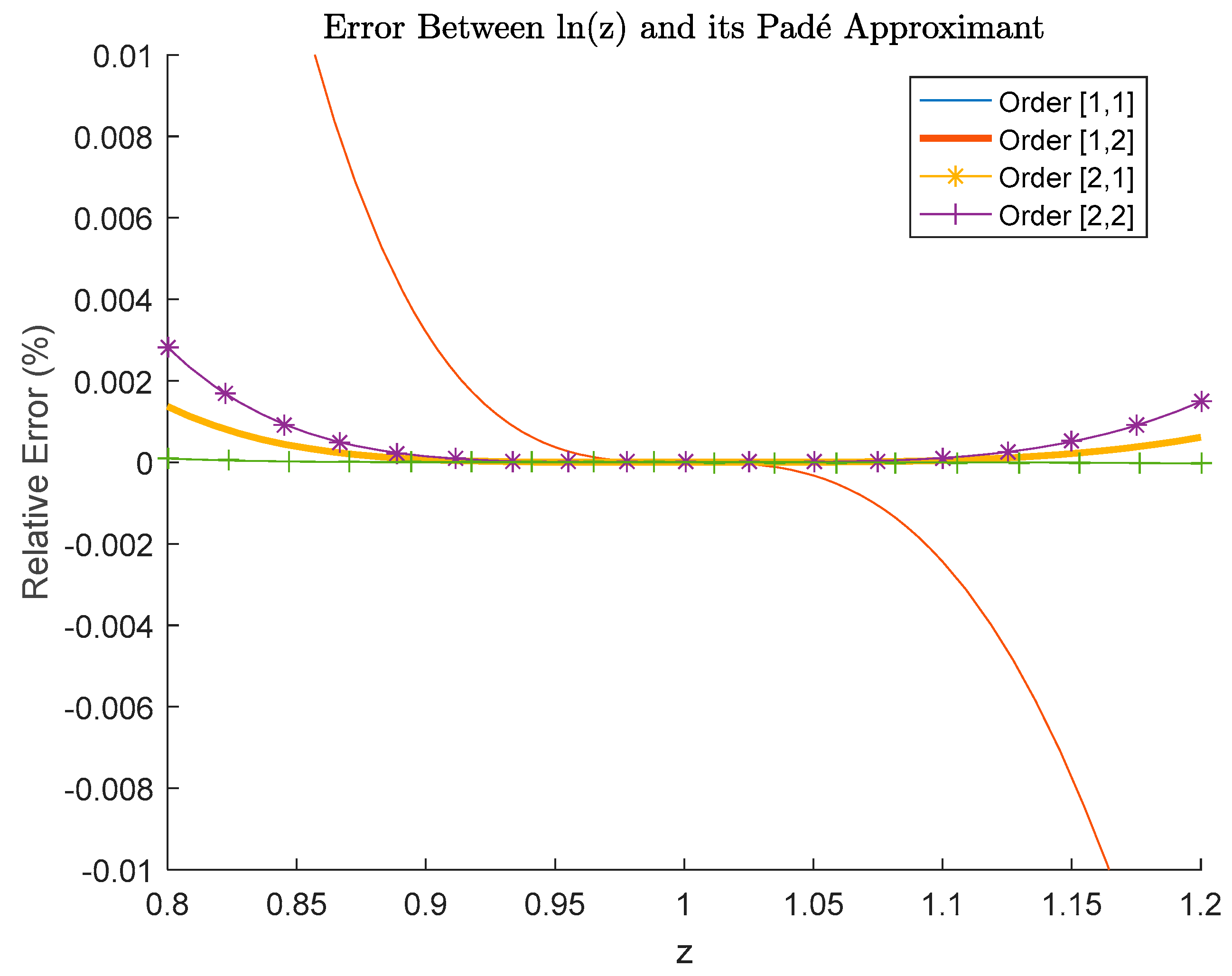
Horner algorithm transforms polynomials into a computationally efficient form and therefore, Horner nested polynomial representations of the Padé polynomials of different orders for $\mathit{ln}\left(z\right)$ where $z\to 1$ are shown here; Equations (2)–(7). Relative error introduced by them; Equations (2)–(5) compared with $\mathit{ln}\left(z\right)$ is shown in Figure 1 and for Equation (6) in

Table 1. Relative error in % of Padé approximant (2,3) for z in interval [0.6; 1,6].

z	${\mathit{log}}_{\mathbf{10}}\mathbf{\left(}\mathit{z}\mathbf{\right)}\mathbf{=}\frac{\mathit{ln}\mathbf{\left(}\mathit{z}\mathbf{\right)}}{\mathit{ln}\mathbf{\left(}\mathbf{10}\mathbf{\right)}}$	Padé Approximants (2,3)	Relative Error %
0.6	−0.22184875	−0.221847398	6.1 × 10−4%
0.65	−0.187086643	−0.187086228	2.2 × 10−4%
0.7	−0.15490196	−0.154901848	7.2 × 10−5%
0.75	−0.124938737	−0.124938712	2.0 × 10−5%
0.8	−0.096910013	−0.096910009	4.4 × 10−6%
0.85	−0.070581074	−0.070581074	6.6 × 10−7%
0.9	−0.045757491	−0.045757491	4.9 × 10−8%
0.95	−0.022276395	−0.022276395	6.5 × 10−10%
1	0	0	0%
1.05	0.021189299	0.021189299	4.8 × 10−10%
1.1	0.041392685	0.041392685	2.7 × 10−8%
1.15	0.06069784	0.06069784	2.7 × 10−7%
1.2	0.079181246	0.079181245	1.3 × 10−6%
1.25	0.096910013	0.096910009	4.4 × 10−6%
1.3	0.113943352	0.113943339	1.2 × 10−5%
1.35	0.130333768	0.130333735	2.6 × 10−5%
1.4	0.146128036	0.146127961	5.1 × 10−5%
1.45	0.161368002	0.161367854	9.2 × 10−5%
1.5	0.176091259	0.176090987	1.5 × 10−4%
1.55	0.190331698	0.190331231	2.5 × 10−4%
1.6	0.204119983	0.204119223	3.7 × 10−4%

. Higher order of Padé approximants are more accurate, but more complex. For example, Padé polynomial of order (2,3) is with polynomial of order 2 in numerator and of order 3 in denominator; Equation (6). Of course, low order formulas are simpler, but they have larger errors than high order formulas and vice versa.

Order (1,1), Equation (2):

$$\mathit{ln}\left(z\right)\approx \frac{z·\left(z+4\right)-5}{4·z+2}$$

(2)

Order (1,2), Equation (3):

$$\mathit{ln}\left(z\right)\approx \frac{3·\left(z-1\right)·\left(z+1\right)}{z·\left(z+4\right)+1}$$

(3)

Order (2,1), Equation (4):

$$\mathit{ln}\left(z\right)\approx \frac{-z·\left(z·\left(z-9\right)-9\right)-17}{18·z+6}$$

(4)

Order (2,2), Equation (5):

$$\mathit{ln}\left(z\right)\approx \frac{z·\left(z·\left(z+18\right)-9\right)-10}{z·\left(9·z+18\right)+3}$$

(5)

Order (2,3), Equation (6):

$$\mathit{ln}\left(z\right)\approx \frac{\left(z-1\right)·\left(11·z^2+38·z+11\right)}{3·\left(z^3+9·z^2+9·z+1\right)}$$

(6)

Order (3,2), Equation (7):

$$\mathit{ln}\left(z\right)\approx \frac{z·\left(z·\left(11·z+27\right)-27\right)-11}{z·\left(z·\left(3·z+27\right)+27\right)+3}$$

(7)

In Equations (2)–(7), $z$ is from $z_{01}=\frac{y_0}{y_1}$, $z_{02}=\frac{y_0}{y_2}$, $z_{03}=\frac{y_0}{y_3}$, etc., or $z_{01}=\frac{y_0}{y_1}$, $z_{12}=\frac{y_1}{y_2}$, $z_{23}=\frac{y_2}{y_3}$, etc.; and $y=\frac{2.51·x}{Re}+\frac{{\epsilon }^{*}}{3.71}$.

Relative error of Padé approximants (2,2) for $z\approx 1$ of $ln\left(z\right)$ is negligible for $0.8<z<1.2$. Thus, relative error of the used Padé approximants (2,3) of $ln\left(z\right)$ in the proposed iterative procedure is even more negligible and therefore it is not presented in Figure 1, but it is available in Table 1. As can be seen from Figure 1, even the very simple form of Padé polynomials (1,2) and (2,1) are of high accuracy in respect of domain of interest for solving the Colebrook equation which is z ≈ 1; $z ϵ\left[0.9, 1.1\right]$.

3. Initial Starting Point for the Proposed Iterative Method

In the case of the Colebrook equation, practical experience shows that trying to get a good initial starting point $x_0$ has limited value until it is chosen in the domain of applicability of the equation which is $3.68<x<12.47$. Every initial starting point $x_0$ chosen from the domain of applicability of the Colebrook equation will lead to the final accurate solution surely, with the only difference that in some cases more additional iterations would be needed. Usually, with the initial guess $x_0$ that is close to the exact solution, the iterative procedure converges to it in five or fewer iterations. To date, cases which lead to divergence, fluctuation, or convergence to a possible far away solution outside of the practical domain of applicability of the Colebrook equation are not known. In the proposed approach, a good starting point should be chosen within the domain of applicability of the Colebrook equation and should not contain any logarithmic function and/or non-integer power term.

A number of options to choose an optimal starting point $x_0$ are considered: (1) special case of the Colebrook equation when $Re\to \infty$, (2) integration of the Colebrook equation, (3) explicit approximations of the Colebrook equation, and (4) fixed value.

1.

The common approach is to choose an initial starting point from the zone of fully developed turbulent rough hydraulic flow $x_0=-2·{\mathit{log}}_{10}\left(\frac{{\epsilon }^{*}}{3.71}\right)$, because in this special case of the Colebrook equation where $Re\to \infty$, the equation is in explicit form with respect to $x$; $x_0=\xi \left({\epsilon }^{*}\right)$, where $\xi$ is functional symbol [18,22]. Here the goal is to avoid use of logarithmic functions and therefore, this starting point is not suitable.

2.

An efficient procedure for finding a sufficiently good initial starting point $x_0$ is proposed by Yun [35] in the integral form; Equation (8):

$$x_0=\frac{1}{2}·\left\{a+b+sgn\left(F\left(a\right)\right)·{\int }_a^b\tanh \left(F\left(x\right)\right)dx\right\}$$

(8)

In Equation (8), $F=x-\xi \left(x\right)=0$, $\xi$ represents the Colebrook equation, $a$ is the lower while $b$ is the upper limit from which an initial starting point $x_0$ should be chosen; $a$ = 3.68 and $b$ = 12.47 because the domain of applicability of the Colebrook equation that is between 3.68 and 12.47 in respect to $x$, $sgn$ is signum function: if $F\left(a\right)>0\to \mathit{sgn}\left(F\left(a\right)\right)=1$, $F\left(a\right)=0\to \mathit{sgn}\left(F\left(a\right)\right)=0$, and $F\left(a\right)<0\to \mathit{sgn}\left(F\left(a\right)\right)=-1$, while $tanh$ is hyperbolic tangent which is defined through the exponential function $e^x$ with non-integer power $x$ the use of which is as computationally expensive as the use of the logarithmic function and which therefore cannot be recommended.

3.

Every explicit approximation of the Colebrook equation [19,20,21,22,23,24,25,26,27,28]; $x\approx \varsigma \left(Re,{\epsilon }^{*}\right)$, where $\varsigma$ is the functional symbol, can be used to choose an initial starting point $x_0$. On the other hand, almost all available approximations contain logarithmic or/and terms with non-integer powers, which makes them unsuitable for use in the developed approach. On the other hand, having previous experience with training Artificial Neural Networks (ANN) to simulate the Colebrook equation [36], i.e., to use ability of artificial intelligence to simulate the Colebrook equation not knowing its logarithmic nature but only knowing raw input and corresponding output datasets $\left\{Re, {\epsilon }^{*}\right\}\to \left\{x\right\}$, a computationally cheap explicit approximation of the Colebrook equation is developed through genetic programming [21,37,38,39,40]. The developed approximation is computationally efficient because of its polynomial structure; Equation (9):

$$x_0=5.05-30.73·{\epsilon }^{*}+\frac{3.4·Re+\frac{R{e}^2}{469647.7}}{46137.9+Re+\frac{R{e}^2}{3250657.6}+\frac{{\epsilon }^{*}·R{e}^2}{515.25}}$$

(9)

Eureqa [computer software] by Nutonian, Inc., Boston, MA, USA. [41,42] is used to generate Equation (9). The Eureqa-polynomial approximation; Equation (9) has up to 40% relative error, but it is very cheap and sufficiently accurate to serve as an initial starting point $x_0$.

4.

Extensive tests over the domain of applicability of the Colebrook equation shows that one fixed value can also be used as the initial starting point $x_0$ for the iterative procedure in all cases. Results indicate that the proposed Padé approach works in all cases, as the argument z of ln(z) is always close to one. When Equation (9) is used, values of z are within the range 0.91–1.05. Moreover, for the most pairs of the Reynolds number $Re$ and the relative roughness of inner pipe surfaces ${\epsilon }^{*}$ which are in the domain of applicability, the initial starting point $x_0=7.273124147$ requires the least number of iterations.

To avoid using a computationally expensive logarithmic function in the initial stage of the iterative procedure, the recommendation is to start calculation with fixed-value starting point $x_0=7.273124147$ or to use a polynomial expression; Equation (9). Power-law formulas from Russian practice which does not contain logarithmic function can also be used as an alternative although they usually contain integer power in fractional form [43,44,45].

4. Proposed Iterative Method

The Colebrook equation is usually solved iteratively using the Newton-Raphson method [46] or even more using a simplified Newton-Raphson method known as the fixed-point method [18]. Recently, hybrid three-point methods have been proposed [47,48].

Here is presented an adjusted very accurate, fast and computationally cheap version of the Newton-Raphson method suitable for the Colebrook equation in which the logarithmic function is replaced after the first iteration with the Padé approximant in polynomial form [29].

Knowing that the Colebrook equation is based on logarithmic law [1,2], the achievement with this simplified approach is more significant. Numerical examples are shown in Section 5 of this paper.

Iteration 0:

In order to avoid use of computationally expensive logarithmic functions or functions with non-integer powers, a required initial starting point $x_0$ should be chosen using recommendations from Section 3 of this paper; points 3 or 4.

Iteration 1:

Having provided an initial starting point $x_0$, new value $x_1$ can be calculated using Equation (10):

$$x_1=x_0-\frac{F\left(x_0\right)}{F^{\prime }\left(x_0\right)}$$

(10)

In Equation (10), $F\left(x\right)$ represents the Colebrook equation $x=\xi \left(x\right)$ which needs to be in suitable form, $F=x-\xi \left(x\right)=0$; Equation (11):

$$F\left(x_0\right)=x_0+2·{\mathit{log}}_{10}\left(y_0\right)=0$$

(11)

In Equation (11), $y_0=\frac{2.51·x_0}{Re}+\frac{{\epsilon }^{*}}{3.71}$ which will also be used in the next iteration (in an additional variant of the proposed method $y_0$ is used in all subsequent iterations), while in Equation (10), the first derivative of $F$ in respect to $x$; $F^{\prime }\left(x\right)$ is from Equation (12):

$$F^{\prime }\left(x_0\right)=1+\frac{2·2.51}{2.302585093·Re·\left(\frac{100·{\epsilon }^{*}}{371}+\frac{2.51·x_0}{Re}\right)}$$

(12)

In Equation (12), $ln\left(10\right)\approx 2.302585093$ is with constant value, and therefore only ${log}_{10}\left(y_0\right)$ from Equation (11) requires evaluation of the logarithmic function.

In many programming languages, evaluation of logarithmic function of any base is processed by natural logarithm [14]. Change of 10-base logarithm from the Colebrook equation to e-based natural logarithm where $e\approx 2.718$ and where $\mathit{ln}\left(10\right)\approx 2.302585093$ is implemented as ${\mathit{log}}_{10}\left(z\right)=\frac{\mathit{ln}\left(z\right)}{\mathit{ln}\left(10\right)}$.

Iteration 2:

New value $x_2$ should be calculated using Equation (13):

$$x_2=x_1-\frac{F\left(x_1\right)}{F^{\prime }\left(x_1\right)}$$

(13)

In Equation (13), $F\left(x_1\right)$ is not calculated by ${\mathit{log}}_{10}\left(y_1\right)$, where $y_1=\frac{2.51·x_1}{Re}+\frac{{\epsilon }^{*}}{3.71}$, but using Padé polynomial replacement for logarithmic function which is accurate for $z\to 1$ and using the already calculated value of ${\mathit{log}}_{10}\left(y_0\right)$ from the previous iteration; Equation (14):

$$F\left(x_1\right)=x_1+2·{\mathit{log}}_{10}\left(y_0\right)-\frac{\left(z_{01}-1\right)·\left(11·z_{01}^2+38·z_{01}+11\right)}{2.302585093·\left(3·z_{01}^3+9·z_{01}^2+9·z_{01}+1\right)}$$

(14)

In Equation (14), ${\mathit{log}}_{10}\left(y_0\right)-\frac{\left(z_{01}-1\right)·\left(11·z_{01}^2+38·z_{01}+11\right)}{2.302585093·\left(3·z_{01}^3+9·z_{01}^2+9·z_{01}+1\right)}\equiv {\mathit{log}}_{10}\left(y_1\right)$, $2.302585093\approx ln\left(10\right)$, and $z_{01}=\frac{y_0}{y_1}$. In the first iteration, ${\mathit{log}}_{10}\left(y_0\right)$ is already known; Equation (11). The Padé polynomial used in Equation (14) is of order (2,3) which means that the polynomial in the numerator is of the order of 2 while in the denominator of order 3. The Padé polynomials are also known as Padé approximants and here the maximal relative error of the polynomial expression term in Equation (14) in domain $zϵ\left[0.6,1.6\right]$; $z\to 1$ is minor as shown in Table 1. Value of z for the procedure shown in practice is $zϵ\left[0.9,1.1\right]$ and therefore the error of the used Padé approximant can be neglected in the case shown.

The first derivative $F^{\prime }\left(x_1\right)$ does not contain any logarithmic functions and should be evaluated using Equation (12), where $x_0$ should be replaced with the new value $x_1$ or knowing that the value of the derivative does not change significantly between two iterations, $F^{\prime }\left(x_0\right)$ can be reused in all subsequent iterative cycles. Even knowing that the value of the first derivate in the procedure shown is always near 1; for rough calculations it can be assumed that $F^{\prime }\left(x\right)\approx 1$ which gives the fixed-point method as a special case of the Newton-Raphson scheme.

Iteration 3:

New value $x_3$ is again evaluated in the same way using Equation (15):

$$x_3=x_2-\frac{F\left(x_2\right)}{F^{\prime }\left(x_2\right)}$$

(15)

In Equation (15), $F^{\prime }\left(x_2\right)$ can be calculated or $F^{\prime }\left(x_1\right)$ or $F^{\prime }\left(x_0\right)$ can be reused. In additon, $F\left(x_2\right)$ can be calculated using $z_{02}=\frac{y_0}{y_2}$, where $y_2=\frac{2.51·x_2}{Re}+\frac{{\epsilon }^{*}}{3.71}$. Input parameter for Padé polynomial $z_{02}$ here refers to $y_0$ from the first iteration; Equation (16):

$$F\left(x_2\right)=x_2+2·{\mathit{log}}_{10}\left(y_0\right)-\frac{\left(z_{02}-1\right)·\left(11·z_{02}^2+38·z_{02}+11\right)}{2.302585093·\left(3·z_{02}^3+9·z_{02}^2+9·z_{02}+1\right)}$$

(16)

In Equation (16), ${\mathit{log}}_{10}\left(y_0\right)-\frac{\left(z_{02}-1\right)·\left(11·z_{02}^2+38·z_{02}+11\right)}{2.302585093·\left(3·z_{02}^3+9·z_{02}^2+9·z_{02}+1\right)}\equiv {\mathit{log}}_{10}\left(y_2\right)$.

The Padé polynomial is a very accurate approximation of logarithmic function, so knowing that $y_0$ is evaluated directly through the logarithmic function, while $y_1$, $y_2$, $y_3$, etc. is based on its Padé polynomial equivalent, it is obvious that the sequence $z_{01}=\frac{y_0}{y_1}$, $z_{02}=\frac{y_0}{y_2}$, $z_{03}=\frac{y_0}{y_3}$, etc. is slightly more accurate compared with the sequence $z_{01}=\frac{y_0}{y_1}$, $z_{12}=\frac{y_1}{y_2}$, $z_{23}=\frac{y_2}{y_3}$, etc. which accumulates error introduced with Padé approximations. Anyway, the introduced error is so small that it can practically be neglected. The second sequence $z_{01}=\frac{y_0}{y_1}$, $z_{12}=\frac{y_1}{y_2}$, $z_{23}=\frac{y_2}{y_3}$, etc. yields Equation (17):

$$\begin{gathered} F\left(x_2\right)=x_2+2·{\mathit{log}}_{10}\left(y_1\right)-\frac{\left(z_{12}-1\right)·\left(11·z_{12}^2+38·z_{12}+11\right)}{2.302585093·\left(3·z_{12}^3+9·z_{12}^2+9·z_{12}+1\right)}=x_2+ \\ 2·{\mathit{log}}_{10}\left(y_0\right)-\frac{\left(z_{01}-1\right)·\left(11·z_{01}^2+38·z_{01}+11\right)}{2.302585093·\left(3·z_{01}^3+9·z_{01}^2+9·z_{01}+1\right)}-\frac{\left(z_{12}-1\right)·\left(11·z_{12}^2+38·z_{12}+11\right)}{2.302585093·\left(3·z_{12}^3+9·z_{12}^2+9·z_{12}+1\right)} \end{gathered}$$

(17)

In Equation (17), ${\mathit{log}}_{10}\left(y_1\right)-\frac{\left(z_{12}-1\right)·\left(11·z_{12}^2+38·z_{12}+11\right)}{2.302585093·\left(3·z_{12}^3+9·z_{12}^2+9·z_{12}+1\right)}\equiv {\mathit{log}}_{10}\left(y_2\right)$ and, ${\mathit{log}}_{10}\left(y_0\right)-\frac{\left(z_{01}-1\right)·\left(11·z_{01}^2+38·z_{01}+11\right)}{2.302585093·\left(3·z_{01}^3+9·z_{01}^2+9·z_{01}+1\right)}\equiv {\mathit{log}}_{10}\left(y_1\right)$

Iteration i:

All indexes $i$ in respect the third iteration should be updated as $i=i+1$ with exemption of index 0 in Equation (16). The calculation is finished when $x_{i+1}\approx x_i$.

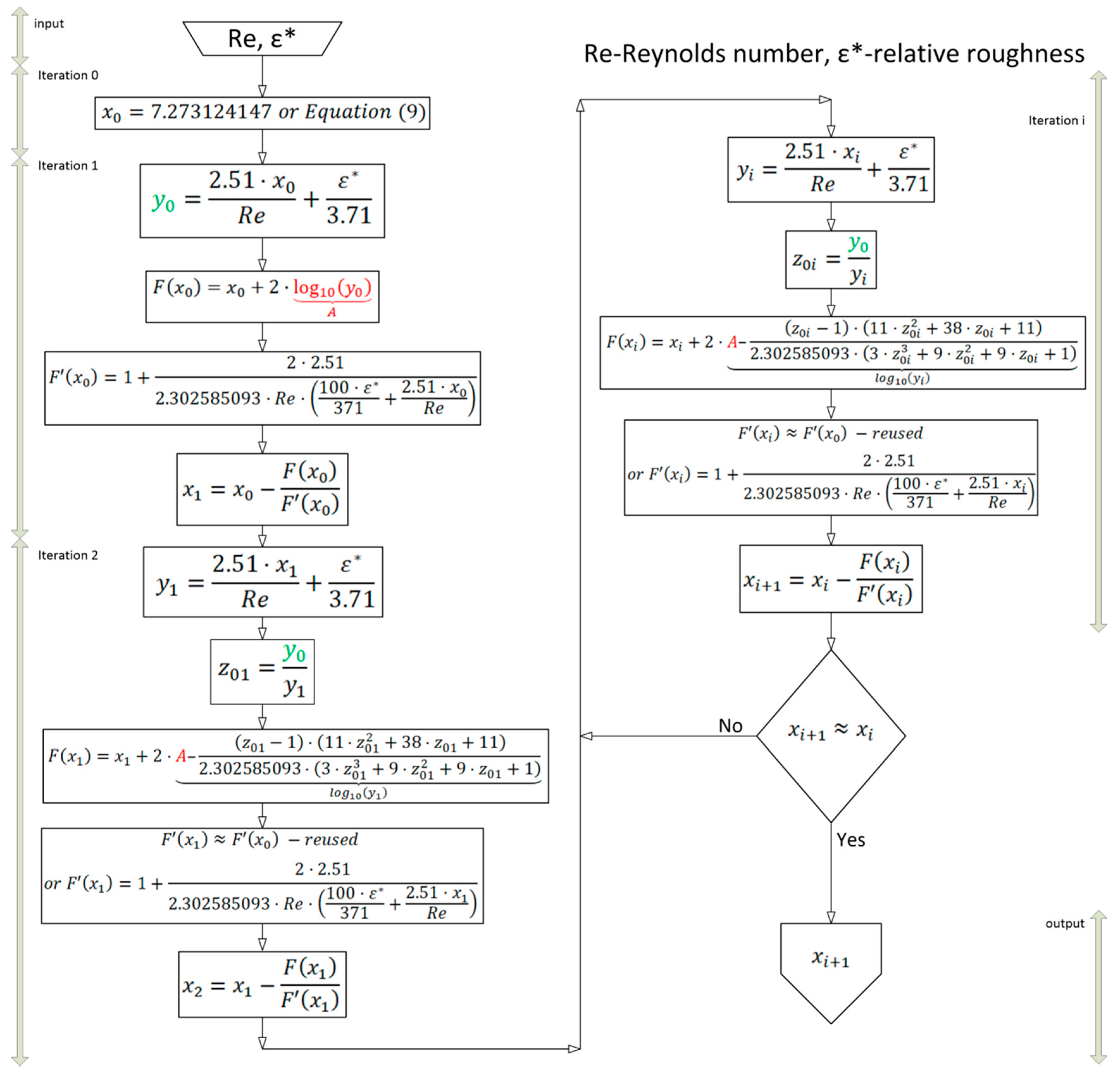
The algorithm for the proposed improved procedure is given in Figure 2.

Only a one-off evaluation of the logarithmic function is needed in the proposed algorithm from Figure 2, which is clearly marked in red; $A={log}_{10}\left(y_0\right)$. On the other hand, $y_0$ calculated in iteration 1 is reused in all next steps and it is marked in green in Figure 2.

The proposed procedure can be simplified assuming that $F^{\prime }\left(x_i\right)=1$, which gives the simple fixed-point procedure [18] instead of the Newton-Raphson.

5. Numerical Examples

Here are two numerical examples:

Example 1:	Example 2:
$Re=8.31·{10}^3$, ${\epsilon }^{*}=0.024$	$Re=2.5·{10}^6$, ${\epsilon }^{*}=4·{10}^{-4}$
Iteration 0
$x_0=6.279860788$	$x_0=7.401979091$	(9)
Iteration 1
$y_0=0.008365808$	$y_0=0.000115248$
${\mathit{log}}_{10}\left(y_0\right)=-2.077492116$	${\mathit{log}}_{10}\left(y_0\right)=-3.938365477$
$F\left(x_0\right)=2.124876556$	$F\left(x_0\right)=-0.474751864$	(11)
$F^{\prime }\left(x_0\right)=1.001337518$	$F^{\prime }\left(x_0\right)=1.001024781$	(12)
$x_1=4.157822498$	$x_1=7.876244936$	(10)
Iteration 2
$y_1=0.007724855$	$y_1=0.000115724$
$z_{01}=\frac{y_0}{y_1}=1.082972765$	$z_{01}=\frac{y_0}{y_1}=0.995885374$
0.034617535	−0.001790646	Padé approximant (6)
$F\left(x_1\right)=-0.066396805$	$F\left(x_1\right)=0.003095273$	(14)
$F{F}^{\prime }\left(x_1\right)=1.001986711$	$F^{\prime }\left(x_1\right)=1.000970478$
$x_2=4.224087653$	$x_2=7.873152664$	(13)
Iteration 3
$y_2=0.00774487$	$y_2=0.000115721$
$z_{02}=\frac{y_0}{y_2}=1.080174034$	$z_{02}=\frac{y_0}{y_2}=0.995912092$
0.033493733	−0.001778995	Padé approximant (6)
$F\left(x_2\right)=0.002115955$	$F\left(x_2\right)=-2.03017·{10}^{-5}$	(16)
$F^{\prime }\left(x_2\right)=1.001957048$	$F^{\prime }\left(x_2\right)=1.000970813$
$x_3=4.221975832$	$x_3=7.873172946$	(15)
Final value:
$x$ = 4.22204103	$x$ = 7.873172814
$\lambda =\frac{1}{x^2}=0.056098998$	$\lambda =\frac{1}{x^2}=0.016132454$

Example 1:	Example 2:
$Re=8.31·{10}^3$, ${\epsilon }^{*}=0.024$	$Re=2.5·{10}^6$, ${\epsilon }^{*}=4·{10}^{-4}$
Iteration 0
$x_0=6.279860788$	$x_0=7.401979091$	(9)
Iteration 1
$y_0=0.008365808$	$y_0=0.000115248$
${\mathit{log}}_{10}\left(y_0\right)=-2.077492116$	${\mathit{log}}_{10}\left(y_0\right)=-3.938365477$
$F\left(x_0\right)=2.124876556$	$F\left(x_0\right)=-0.474751864$	(11)
$F^{\prime }\left(x_0\right)=1.001337518$	$F^{\prime }\left(x_0\right)=1.001024781$	(12)
$x_1=4.157822498$	$x_1=7.876244936$	(10)
Iteration 2
$y_1=0.007724855$	$y_1=0.000115724$
$z_{01}=\frac{y_0}{y_1}=1.082972765$	$z_{01}=\frac{y_0}{y_1}=0.995885374$
0.034617535	−0.001790646	Padé approximant (6)
$F\left(x_1\right)=-0.066396805$	$F\left(x_1\right)=0.003095273$	(14)
$F{F}^{\prime }\left(x_1\right)=1.001986711$	$F^{\prime }\left(x_1\right)=1.000970478$
$x_2=4.224087653$	$x_2=7.873152664$	(13)
Iteration 3
$y_2=0.00774487$	$y_2=0.000115721$
$z_{02}=\frac{y_0}{y_2}=1.080174034$	$z_{02}=\frac{y_0}{y_2}=0.995912092$
0.033493733	−0.001778995	Padé approximant (6)
$F\left(x_2\right)=0.002115955$	$F\left(x_2\right)=-2.03017·{10}^{-5}$	(16)
$F^{\prime }\left(x_2\right)=1.001957048$	$F^{\prime }\left(x_2\right)=1.000970813$
$x_3=4.221975832$	$x_3=7.873172946$	(15)
Final value:
$x$ = 4.22204103	$x$ = 7.873172814
$\lambda =\frac{1}{x^2}=0.056098998$	$\lambda =\frac{1}{x^2}=0.016132454$

6. Conclusions

An efficient algorithm for the iterative calculation of the Colebrook equation by both an accurate and computationally efficient Padé approximation is presented in this paper. It requires only one evaluation of the logarithmic function in respect to the whole iterative procedure and more specifically only in the first iteration, while the common procedures from current engineering practice require at least one evaluation of logarithmic function for every single iteration. The logarithmic function in the proposed procedure is replaced in all iterations (except the first), with simple, accurate and efficient Padé polynomials [29]. In this way the same accuracy is reached through the proposed less demanding procedure, after the same number of iterations as in the standard algorithm which uses $log$-call in each iterative step. This is a good achievement, knowing that the nature of the Colebrook equation is logarithmic. For their evaluation in the Central Processor Unit (CPU), Padé polynomials require a lower number of floating-point operations to be executed compared with the logarithmic function [10,11,12,13,14,30,31,32,33,34,44].

The here presented iterative approach only introduces a computationally cheaper alternative to the standard iterative procedure. It does not reduce the number of required iterations to reach the final desired accuracy nor provide more accurate results. The proposed method reduces the burden for the Central Processor Unit (CPU) as less floating-point operations need to be executed. In that way, the presented approach also increases speed of computation. On the other hand, many explicit non-iterative approximations to the Colebrook equation are available in literature [19,20,21,22,23,24,25,26,27,28,49] which initially appear simple for computation, but are not. They are widely used, but although some of them are very accurate, they contain relatively complex internal iterative steps and also a number of computationally demanding functions. For example, the widely used Haaland approximation [49,50] introduces relative error up to 1.5%, but with the cost of evaluation of one logarithmic expression and one non-integer power. In addition, the approximation by Romeo et al. [26,39] reaches extremely high accuracy with the relative error of up to 0.14%, but with a cost of evaluation of even three logarithmic expressions and two non-integer powers. Regarding alternative iterative procedures, Clamond [10] provides an accurate iterative approach using $\Omega$ function, but this algorithm requires at least two $log$-calls; one for initialization and one in the first iteration, which is more expensive compared with the here presented approach.

The procedure proposed in this paper can significantly reduce the computational burden for evaluating complex distribution networks with various applications (water, gas) [9,50,51,52,53,54,55]. For example, a probabilistic approach using time dependent modeling of distribution or transmission networks requires many millions of evaluations of Colebrook’s equation. For such kinds of computations it is always good to have a cheaper but still accurate approach to speed up the process.

References

- Colebrook, C.F. Turbulent flow in pipes with particular reference to the transition region between the smooth and rough pipe laws. J. Inst. Civ. Eng. (Lond.) 1939, 11, 133–156. [Google Scholar] [CrossRef]
- Colebrook, C.; White, C. Experiments with fluid friction in roughened pipes. Proc. R. Soc. Lond. Ser. A Math. Phys. Sci. 1937, 161, 367–381. [Google Scholar] [CrossRef] [Green Version]
- Moody, L.F. Friction factors for pipe flow. Trans. ASME 1944, 66, 671–684. [Google Scholar]
- LaViolette, M. On the history, science, and technology included in the Moody diagram. J. Fluids Eng. 2017, 139, 030801. [Google Scholar] [CrossRef]
- Flack, K.A. Moving beyond Moody. J. Fluid Mech. 2018, 842, 1–4. [Google Scholar] [CrossRef] [Green Version]
- Allen, J.J.; Shockling, M.A.; Kunkel, G.J.; Smits, A.J. Turbulent flow in smooth and rough pipes. Philos. Trans. R. Soc. Lond. A Math. Phys. Eng. Sci. 2007, 365, 699–714. [Google Scholar] [CrossRef] [PubMed] [Green Version]
- Langelandsvik, L.I.; Kunkel, G.J.; Smits, A.J. Flow in a commercial steel pipe. J. Fluid Mech. 2008, 595, 323–339. [Google Scholar] [CrossRef]
- McKeon, B.J.; Zagarola, M.V.; Smits, A.J. A new friction factor relationship for fully developed pipe flow. J. Fluid Mech. 2005, 538, 429–443. [Google Scholar] [CrossRef]
- Praks, P.; Kopustinskas, V.; Masera, M. Monte-Carlo-based reliability and vulnerability assessment of a natural gas transmission system due to random network component failures. Sustain. Resil. Infrastruct. 2017, 2, 97–107. [Google Scholar] [CrossRef]
- Clamond, D. Efficient resolution of the Colebrook equation. Ind. Eng. Chem. Res. 2009, 48, 3665–3671. [Google Scholar] [CrossRef]
- Giustolisi, O.; Berardi, L.; Walski, T.M. Some explicit formulations of Colebrook–White friction factor considering accuracy vs. computational speed. J. Hydroinform. 2011, 13, 401–418. [Google Scholar] [CrossRef] [Green Version]
- Danish, M.; Kumar, S.; Kumar, S. Approximate explicit analytical expressions of friction factor for flow of Bingham fluids in smooth pipes using Adomian decomposition method. Commun. Nonlinear Sci. Numer. Simul. 2011, 16, 239–251. [Google Scholar] [CrossRef]
- Winning, H.K.; Coole, T. Explicit friction factor accuracy and computational efficiency for turbulent flow in pipes. Flow Turbul. Combust. 2013, 90, 1–27. [Google Scholar] [CrossRef]
- Vatankhah, A.R. Approximate analytical solutions for the Colebrook equation. J. Hydraul. Eng. 2018, 144, 06018007. [Google Scholar] [CrossRef]
- Sonnad, J.R.; Goudar, C.T. Constraints for using Lambert W function-based explicit Colebrook–White equation. J. Hydraul. Eng. 2004, 130, 929–931. [Google Scholar] [CrossRef]
- Brkić, D. Comparison of the Lambert W-function based solutions to the Colebrook equation. Eng. Comput. 2012, 29, 617–630. [Google Scholar] [CrossRef]
- Brkić, D. W solutions of the CW equation for flow friction. Appl. Math. Lett. 2011, 24, 1379–1383. [Google Scholar] [CrossRef]
- Brkić, D. Solution of the implicit Colebrook equation for flow friction using Excel. Spreadsheets Educ. (eJSiE) 2017, 10, 2. Available online: http://epublications.bond.edu.au/ejsie/vol10/iss2/2 (accessed on 11 July 2018).
- Gregory, G.A.; Fogarasi, M. Alternate to standard friction factor equation. Oil Gas J. 1985, 83, 120–127. [Google Scholar]
- Brkić, D. Review of explicit approximations to the Colebrook relation for flow friction. J. Pet. Sci. Eng. 2011, 77, 34–48. [Google Scholar] [CrossRef] [Green Version]
- Brkić, D.; Ćojbašić, Ž. Evolutionary optimization of Colebrook’s turbulent flow friction approximations. Fluids 2017, 2, 15. [Google Scholar] [CrossRef]
- Brkić, D. Determining friction factors in turbulent pipe flow. Chem. Eng. 2012, 119, 34–39. [Google Scholar]
- Buzzelli, D. Calculating friction in one step. Mach. Des. 2008, 80, 54–55. [Google Scholar]
- Zigrang, D.J.; Sylvester, N.D. Explicit approximations to the solution of Colebrook’s friction factor equation. AIChE J. 1982, 28, 514–515. [Google Scholar] [CrossRef]
- Serghides, T.K. Estimate friction factor accurately. Chem. Eng. 1984, 91, 63–64. [Google Scholar]
- Romeo, E.; Royo, C.; Monzón, A. Improved explicit equations for estimation of the friction factor in rough and smooth pipes. Chem. Eng. J. 2002, 86, 369–374. [Google Scholar] [CrossRef]
- Vatankhah, A.R.; Kouchakzadeh, S. Discussion of “Turbulent flow friction factor calculation using a mathematically exact alternative to the Colebrook–White equation” by Jagadeesh R. Sonnad and Chetan T. Goudar. J. Hydraul. Eng. 2008, 134, 1187. [Google Scholar] [CrossRef]
- Vatankhah, A.R.; Kouchakzadeh, S. Discussion of “Exact equations for pipe-flow problems”. J. Hydraul. Res. 2009, 47, 537–538. [Google Scholar] [CrossRef]
- Baker, G.A.; Graves-Morris, P. Padé approximants. In Encyclopedia of Mathematics and Its Applications; Cambridge University Press: Cambridge, UK, 1996. [Google Scholar] [CrossRef]
- Kropa, J.C. Calculator algorithms. Math. Mag. 1978, 51, 106–109. [Google Scholar] [CrossRef]
- Rising, G.R. Inside Your Calculator: From Simple Programs to Significant Insights; John Wiley & Sons: Hoboken, NJ, USA, 2007. [Google Scholar] [CrossRef]
- Pineiro, J.A.; Ercegovac, M.D.; Bruguera, J.D. Algorithm and architecture for logarithm, exponential, and powering computation. IEEE Trans. Comput. 2004, 53, 1085–1096. [Google Scholar] [CrossRef]
- Biberg, D. Fast and accurate approximations for the Colebrook equation. J. Fluids Eng. 2017, 139, 031401. [Google Scholar] [CrossRef]
- Winning, H.K.; Coole, T. Improved method of determining friction factor in pipes. Int. J. Numer. Methods Heat Fluid Flow 2015, 25, 941–949. [Google Scholar] [CrossRef]
- Yun, B.I. A non-iterative method for solving non-linear equations. Appl. Math. Comput. 2008, 198, 691–699. [Google Scholar] [CrossRef]
- Brkić, D.; Ćojbašić, Ž. Intelligent flow friction estimation. Comput. Intell. Neurosci. 2016, 5242596. [Google Scholar] [CrossRef] [PubMed]
- Giustolisi, O.; Savić, D.A. A symbolic data-driven technique based on evolutionary polynomial regression. J. Hydroinform. 2006, 8, 207–222. [Google Scholar] [CrossRef]
- Petković, D.; Gocić, M.; Shamshirband, S. Adaptive Neuro-Fuzzy computing technique for precipitation estimation. Facta Univ. Ser. Mech. Eng. 2016, 14, 209–218. [Google Scholar] [CrossRef]
- Ćojbašić, Ž.; Brkić, D. Very accurate explicit approximations for calculation of the Colebrook friction factor. Int. J. Mech. Sci. 2013, 67, 10–13. [Google Scholar] [CrossRef] [Green Version]
- Mitrev, R.; Tudjarov, B.; Todorov, T. Cloud-based expert system for synthesis and evolutionary optimization of planar linkages. Facta Univ. Ser. Mech. Eng. 2018. [Google Scholar] [CrossRef]
- Schmidt, M.; Lipson, H. Distilling free-form natural laws from experimental data. Science 2009, 324, 81–85. [Google Scholar] [CrossRef] [PubMed]
- Dubčáková, R. Eureqa: Software review. Genet. Program. Evol. Mach. 2011, 12, 173–178. [Google Scholar] [CrossRef] [Green Version]
- Альтшуль, А.Д. Гидравлические Сопротивления; Недра: Moscow, Russia, 1982. (In Russian) [Google Scholar]
- Lipovka, A.Y.; Lipovka, Y.L. Determining hydraulic friction factor for pipeline systems. Journal of Siberian Federal University. Eng. Technol. 2014, 7, 62–82. Available online: http://elib.sfu-kras.ru/handle/2311/10293 (accessed on 11 July 2018).
- Черникин, В.А.; Черникин, А.В. Обобщенная формула для расчета коэффициента гидравлического сопротивления магистральных трубопроводов для светлых нефтепродуктов и маловязких нефтей. Наука и Технологии Трубопроводного Транспорта Нефти и Нефтепродуктов 2012, 4, 64–66. (In Russian) [Google Scholar]
- Abbasbandy, S. Improving Newton–Raphson method for nonlinear equations by modified Adomian decomposition method. Appl. Math. Comput. 2003, 145, 887–893. [Google Scholar] [CrossRef]
- Brkić, D.; Praks, P. Discussion of “Approximate analytical solutions for the Colebrook equation”. J. Hydraul. Eng. 2019, 144, 06018007. [Google Scholar]
- Džunić, J.; Petković, M.S.; Petković, L.D. A family of optimal three-point methods for solving nonlinear equations using two parametric functions. Appl. Math. Comput. 2011, 217, 7612–7619. [Google Scholar] [CrossRef]
- Haaland, S.E. Simple and explicit formulas for the friction factor in turbulent pipe flow. J. Fluids Eng. 1983, 105, 89–90. [Google Scholar] [CrossRef]
- Wood, D.J.; Haaland, S.E. Discussion and closure: “Simple and explicit formulas for the friction factor in turbulent pipe flow” (Haaland, S.E., 1983, ASME J. Fluids Eng., 105, pp. 89–90). J. Fluids Eng. 1983, 105, 242–243. [Google Scholar] [CrossRef]
- Praks, P.; Kopustinskas, V.; Masera, M. Probabilistic modelling of security of supply in gas networks and evaluation of new infrastructure. Reliab. Eng. Syst. Saf. 2015, 144, 254–264. [Google Scholar] [CrossRef]
- Brkić, D. Spreadsheet-based pipe networks analysis for teaching and learning purpose. Spreadsheets Educ. (eJSiE) 2016, 9, 4. Available online: https://epublications.bond.edu.au/ejsie/vol9/iss2/4/ (accessed on 11 July 2018).
- Brkić, D. Discussion of “Economics and statistical evaluations of using Microsoft Excel solver in pipe network analysis” by I.A. Oke, A. Ismail, S. Lukman, S.O. Ojo, O.O. Adeosun, and M.O. Nwude. J. Pipeline Syst. Eng. Pract. 2018, 9, 07018002. [Google Scholar] [CrossRef]
- Brkić, D. Iterative methods for looped network pipeline calculation. Water Resour. Manag. 2011, 25, 2951–2987. [Google Scholar] [CrossRef]
- Brkić, D. A gas distribution network hydraulic problem from practice. Petrol. Sci. Technol. 2011, 29, 366–377. [Google Scholar] [CrossRef]
Figure 1.
Relative error between ln(z) and its Padé approximants accurate for z ≈ 1.
Figure 2.
Algorithm for the proposed one -call improved procedure.