Decoupling Greenhouse Gas Emissions from Crop Production: A Case Study in the Heilongjiang Land Reclamation Area, China

Abstract

Modern agriculture contributes significantly to greenhouse gas emissions in several ways. From the perspective of sustainability assessment, it is not enough to evaluate mitigation measures that rely only on emissions reductions. In this article, we use the method of decoupling analysis to construct a decoupling index based on carbon footprint and crop yield and evaluate the relationship between crop production and greenhouse gas emissions using the most modern grain production base in China as a case study. The results indicate that a weak but variable decoupling trend occurred from 2001 to 2015 and that each branch achieved on average a weak decoupling across the study period. In addition, rice production constituted 80% of the regional carbon footprint in a crop’s life cycle. The results of our analysis of rice production show that weak decoupling was the most common outcome but was not consistent because a weak coupling occurred in 2015. Each branch on average achieved a weak decoupling except for the SH branch. Our research indicates that high agricultural material inputs with low utilization efficiency contributed to the poor relationship between crop production and greenhouse gas emissions in the study area. Fertilizer, especially N fertilizer, was an important contributor to the total greenhouse gas emissions of crop production. As a supplement to carbon footprint assessment, this decoupling analysis helps local decision-makers diagnose the level of green growth, identify key options to mitigate greenhouse gas emissions from agriculture, and adopt more targeted interventions towards sustainable agriculture.

1. Introduction

The relationship between economic growth and environmental pressure has been intensively discussed [1,2,3]. In recent years, green economic growth has attracted worldwide attention as a way to maintain rapid economic development while limiting environmental degradation. Like the term “green economy,” “decoupling” refers to the ability of an economy to grow without a corresponding increase in environmental pressure [4]. Today, decoupling environmental impacts from human well-being has been widely acknowledged by policy-makers, industry leaders, and civil society as a key issue to address in meeting sustainable development goals [5]. In the field of sustainability studies, following the environmental Kuznets curve (EKC) hypothesis [6], decoupling analysis has become increasingly popular, and there is a growing body of literature on the decoupling method and indicators of decoupling [7,8,9,10,11,12]. Indeed, as a policy goal, decoupling environmental impact from economic growth has been adopted by the European Union (EU) and the Green Economy Initiative of the United Nations Environment Program (UNEP) [13].

Climate change is one of the greatest challenges to mankind today. The increases in anthropogenic greenhouse gases (GHGs), including carbon dioxide (CO₂), methane (CH₄), and nitrous oxide (N₂O), have important effects on global warming [14,15]. Many studies have empirically assessed the potential impact of human activities or production sectors on global warming by quantifying the carbon footprint (CF) [16,17,18]. Modern agriculture is usually accompanied by high material inputs, high energy consumption, and high release of pollutants, which all play an important role in GHG emissions [19]. Extensive studies have evaluated agricultural CFs associated with material inputs or based on life cycle assessment (LCA). LCA is a commonly used environmental management tool to assess a product or service from “cradle to grave” [20]. The literature on evaluating the CFs of crop production generally quantified the GHG emissions from sowing to harvest, including the indirect emissions from agricultural material inputs and the direct emissions from energy consumption for farm mechanical operations, N₂O from N fertilizer use or the CH₄ emissions from rice paddies [21,22,23,24]. Studies of CFs for a diverse range of crops have been performed at different geographical scales using national statistical data or farm survey data [17,25,26,27,28], and other studies have described a certain crop’s CF in more detail, such as for rice [29,30,31], spring barley [32], and wheat [33]. In addition, GHG emissions under different cropping systems and farm management practices have been addressed in detail [21,22,23,34,35], and the CFs of crop production have also been compared across countries [27]. All these studies have helped to further explore measures to mitigate agricultural GHG emissions and have put forward potential solutions to develop low-carbon agriculture.

China is a major agricultural producer, and GHG emissions in the agricultural sector account for 17% of the national total [36]. According to previous studies, the CFs of crop production in China [37] were higher than those in the USA [27] and the UK [17] based on national statistical data. From the perspective of sustainability assessment, it is not enough to evaluate mitigation measures depending only on emissions reduction; similarly, it remains difficult to examine if one farming region has taken effective measures to reduce the carbon intensity of agriculture. The Heilongjiang land reclamation area (HLRA) is both the most modern grain production base and the largest green grain production base in China, the application of chemical fertilizers and pesticides in the HLRA is far below the national standard, and its crop yield per unit area exceeds that of the US [38]. However, it is not clear if its high crop yield occurs at the expense of high GHG emissions. In this study, we use this area as an example to estimate the extent to which GHG emissions are decoupled from crop production.

The objectives of this study are, first, to quantify the CFs of crop production (including rice, maize, soybeans, and wheat) using the LCA approach in the HLRA during 2001–2015; second, to determine the relationship between crop production and GHG emissions based on a decoupling index; and, last, to analyze the composition of the CFs of crop production and further provide targeted suggestions for decision-making for low-carbon agriculture.

The flowchart for the decoupling analysis is shown in Figure 1.

2. Materials and Methods

2.1. Carbon Footprint Calculation

The carbon footprint of crop production was expressed in this study in CO₂ equivalents (CE) following the LCA approach. GHG emissions included the direct and indirect emissions from crop production. The indirect emissions were attributed to the manufacture of agricultural material inputs (e.g., fertilizers, pesticides and plastic films) and electricity used for rice irrigation; the direct emissions were attributed to energy consumption from farm mechanical operations including seeding, tillage, transportation and harvesting as well as N₂O from N fertilizer use and CH₄ emissions from rice paddies [25].

GHG emissions from agricultural material inputs or sources were expressed as CF_i (in tCE) using Equation (1):

$$C{F}_i={\displaystyle \sum (I_i\times E{F}_i)},$$

(1)

where I_i is the amount of each agricultural input or source i, including fertilizers (in t), pesticides (in t), seed (in t), plastic films (in t), electricity for rice irrigation (in kWh) and diesel for machinery (in t), and EF_i is the GHG emission factor in this study (

Table 1. Emission factors for agricultural inputs and sources.

Emission Source	Abbreviation	Emission Factor	Reference
Fertilizer	EFf	1.53 tCEt−1 (N fertilizer); 1.63 tCEt−1 (P fertilizer); 0.66 tCEt−1 (K fertilizer)	[30]
Pesticide	EFp	0.20 tCEt−1 (Herbicide); 16.60 tCEt−1 (Insecticide)	[30]
Plastic film	EFpf	22.70 tCEt−1	[30]
Seed	EFs	0.58 tCEt−1	[26]
Electricity for irrigation	EFe	1.23 × 10−3 tCEkWh−1	[26]
Diesel for machinery	EFd	0.89 tCEt−1	[30]
N fertilizer-induced N2O	EFN2O	0.01 tN2O-Nt−1 (Dry cropland); 0.0073 tN2O-Nt−1 (Rice paddy)	[39,40]
CH4 emissions from rice field	EFc	1.30 × 10−3 tCH4 ha−1day−1	[41]
	SFw	0.52	[41]
	SFP	0.68	[41]
	SFm	1	[41]

).

The direct N₂O emissions from fertilizer N use were expressed as CF_N2O (in tCE) using Equation (2):

$$C{F}_{N_{2}O}=I_N\times E{F}_{N_{2}O}\times \frac{44}{28}\times 298,$$

(2)

where I_N represents the amount of N fertilizer used (in t), EF_N2O is the emission factor for N₂O emissions caused by N fertilizer used (in tN₂O-Nt⁻¹) [39,40], 44/28 is the ratio of molecular weights of N₂O to N₂, and 298 is the net global warming potential of N₂O over a 100-year period [40].

The CH₄ emissions from a submerged rice paddy in a single season were expressed as CF_CH4 (in tCE) using Equation (3):

$$C{F}_{C{H}_4}=E{F}_d\times T\times A\times 25,$$

(3)

where EF_d is a daily emission factor (in tCEha⁻¹day⁻¹), T is the rice growing period (in days), A is the planting area (in ha), and 25 is the relative molecular warming forcing of CH₄ in a 100-year period [40].

Here, EF_d was estimated by Equation (4) due to the restricted condition of data:

$$E{F}_d=E{F}_c\times S{F}_w\times S{F}_p\times S{F}_m,$$

(4)

where EF_c is the basic emission factor for fields flooded without organic amendment; SF_w and SF_p are scaling factors for different hydrological conditions over the rice growing period and before rice transplanting, respectively; and SF_m is a scaling factor for quantifying organic amendment used for rice production [41]. All of the above emission factors for agricultural inputs or sources are shown in Table 1.

The total carbon footprint CF_t (in tCE) was calculated for rice production and for dry crop production (maize, soybeans, and wheat) by Equations (5) and (6), respectively:

$$C{F}_t=C{F}_i+C{F}_{N_{2}O}+C{F}_{C{H}_4}$$

(5)

$$C{F}_t=C{F}_i+C{F}_{N_{2}O}.$$

(6)

Based on the estimated CF_t, carbon intensity in crop yield, CF_Y (in tCEt⁻¹), and the carbon intensity in crop area, CF_A (in tCEha⁻¹), were calculated using Equations (7) and (8), respectively, in terms of crop yield (Y, in t) and crop planting area (A, in ha).

$$C{F}_Y=\frac{C{F}_t}{Y}$$

(7)

$$C{F}_A=\frac{C{F}_t}{A}$$

(8)

2.2. Decoupling Index

In this article, the decoupling index (DI) is used to indicate the degree of decoupling of GHG emissions from crop production, following Equation (9):

DI = %ΔCF/%ΔY = (CF_j/CF_j−1 − 1)/(Y_j/Y_j−1 − 1),

(9)

where %ΔCF is the percentage change in GHG emissions from crop production, and CF_j and CF_j−1 denote GHG emissions in a target year j and the base year j − 1; %ΔY is the percentage change in crop yield, and Y_j and Y_j−1 denote the crop yield in a target year j and the base year j − 1, respectively. Six decoupling index values are shown in

Table 2. Degrees of decoupling GHG emissions from crop production.

Decoupling Degree	Relationship between GHG Emissions and Crop Production
Strong decoupling	ΔY > 0, ΔCF ≤ 0, DI ≤ 0
Weak decoupling	ΔY > 0, ΔCF > 0, 0 < DI < 1
Recessive decoupling	ΔY < 0, ΔCF < 0, DI ≥ 1
Expansive coupling	ΔY > 0, ΔCF > 0, DI ≥ 1
Weak coupling	ΔY < 0, ΔCF < 0, 0 < DI < 1
Strong coupling	ΔY < 0, ΔCF ≥ 0, DI ≤ 0

.

2.3. Study Area and Data Sources

The HLRA is located in northeast China and includes nine branches with an area of 57,600 km² (Figure 2). There are four main grain crops in the study area: rice, maize, soybeans, and wheat. Rice and maize are main crops generally grown in the humid eastern branches, whereas soybeans and wheat are the main crops grown in the semi-humid western branches. These four crops accounted for 97% of the total output in 2015. The comprehensive utilization rate of agricultural mechanization is over 94%, and these commodity grains achieve 91% of their annual crop yield in the HLRA, which has improved national food security.

Data for quantifying GHG emissions from agricultural inputs or sources were collected from the National Cost-Benefit Survey for Agricultural Products (2001–2015). Crop yield and planting area data were collected from the Statistical Yearbook of the Heilongjiang Land Reclamation Area (2002–2016), and data for quantifying CH₄ emissions from the rice paddy, including the rice cultivation and growing periods, were obtained from field research and existing literature [26,30,39,40,41].

3. Results and Analysis

3.1. Relationship between Crop Yield and Carbon Footprint

The changes in the crop yields and the CFs of four crops in the HLRA (2001–2015) are shown in Figure 3; the correlation coefficient, R, between crop yield and the CF was 0.994 at a significance level of 0.01. Using crop yield as the independent variable, x, and the CF as the dependent variable, y, the best-fit linear equation relating these two variables was y = 0.2227x + 72.383. The R² and adjusted R² values of this equation were 0.988 and 0.987, respectively, which indicated a close relationship between GHG emissions and crop production in the HLRA.

3.2. Decoupling GHG Emissions from Crop Production

According to Table 2, the results of decoupling GHG emissions from crop production during 2001–2015 in the HLRA are shown in

Table 3. Decoupling GHG emissions from crop production in the HLRA.

Year	Crop Yield (104 t)	Growth Rate of Crop Yield (%)	CF (104 tCE)	Growth Rate of CF (%)	DI	Decoupling Degree
2001	832.17	-	255.72	-	-
2002	761.31	−8.52	254.98	−0.29	0.03	Weak coupling
2003	717.41	−5.77	226.22	−11.28	1.95	Recessive decoupling
2004	901.22	25.62	262.11	15.87	0.62	Weak decoupling
2005	973.10	7.98	275.83	5.23	0.66	Weak decoupling
2006	1065.11	9.46	316.12	14.61	1.54	Expansive coupling
2007	1210.07	13.61	360.04	13.89	1.02	Expansive coupling
2008	1337.51	10.53	381.27	5.9	0.56	Weak decoupling
2009	1631.90	22.01	415.27	8.92	0.41	Weak decoupling
2010	1794.78	9.98	467.96	12.69	1.27	Expansive coupling
2011	2014.16	12.22	512.72	9.56	0.78	Weak decoupling
2012	2085.14	3.52	560.7	9.36	2.66	Expansive coupling
2013	2109.67	1.18	559.8	−0.16	−0.14	Strong decoupling
2014	2165.06	2.63	542.11	−3.16	−1.2	Strong decoupling
2015	2146.15	−0.87	537.46	−0.86	0.99	Weak coupling

, and the results based on the average value in the period 2001–2015 are shown in

Table 4. Decoupling GHG emissions from crop production in the HLRA (average of the years 2001–2015).

Branch	Crop Yield (104 t)	Growth Rate of Crop Yield (%)	CF (104 tCE)	Growth Rate of CF (%)	DI	Decoupling Degree
BQL	220.33	6.56	57.72	5.24	0.8	Weak decoupling
HXL	283.32	7.13	70.3	3.67	0.51	Weak decoupling
JSJ	438.37	9.58	125.94	8.72	0.91	Weak decoupling
MDJ	277.5	5.33	73.87	3.71	0.7	Weak decoupling
BA	122.37	11.79	21.5	3.91	0.33	Weak decoupling
JS	93.06	11.15	12.81	1.39	0.12	Weak decoupling
QQH	67.357	9.82	15.56	6.21	0.63	Weak decoupling
SH	41.46	6.72	11.98	3.84	0.57	Weak decoupling
HB	12.68	11.93	4.84	8.37	0.7	Weak decoupling

.

According to Table 3, during 2001–2015, strong decoupling occurred for two years, weak decoupling occurred for five years, and recessive decoupling occurred for one year, which indicated that changes in carbon intensity were variable during this period and largely composed of weak decoupling. GHG emissions of crop production did not increase in proportion with crop yield in the HLRA for 2013 and 2014. Expansive coupling occurred for four years, and weak coupling occurred for two years. One of these weakly increasing years, 2015, followed two years of strong decoupling, which suggests that HLRA continues to face both challenges and opportunities as low-carbon agriculture continues to develop.

According to Table 4, from the perspective of the branch scale, all branches experienced weak decoupling between crop production and GHG emissions when considering the mean change from 2001–2015. This analysis revealed the potential for the HLRA to experience strong decoupling with continued progress.

3.3. Example: Decoupling GHG Emissions from Rice Production

Rice in the HLRA is economically and environmentally important to China, both as the largest green food base and because of its high-quality rice varieties. On average, rice acreage was 48% of the total grain-planting area, and rice accounted for 62% of the total grain yield in the HLRA during 2001–2015. During these years, GHG emissions from rice production accounted for 80% of the total HLRA CF, with maize, soybeans, and wheat contributing 11%, 7%, and 2% to the total CF, respectively. Further results of decoupling GHG emissions from rice production with regard to the whole HLRA and the branch scale over 2001–2015 are shown in

Table 5. Decoupling GHG emissions from rice production in the HLRA.

Year	Rice Yield (104 t)	Growth Rate of Rice Yield (%)	CF of Rice (104 tCE)	Growth Rate of CF of Rice (%)	DI	Decoupling Degree
2001	527.42	-	194.14	-	-
2002	452.77	−14.15	197.92	1.94	−0.14	Strong coupling
2003	424.16	−6.32	165.73	−16.26	2.57	Recessive decoupling
2004	528.62	24.63	195.99	18.26	0.74	Weak decoupling
2005	573.43	8.48	209.58	6.93	0.82	Weak decoupling
2006	682.5	19.02	250.45	19.5	1.03	Expansive coupling
2007	798.07	16.93	288.25	15.09	0.89	Weak decoupling
2008	842.18	5.53	307.51	6.68	1.21	Expansive coupling
2009	927.32	10.11	322.21	4.78	0.47	Weak decoupling
2010	1094.39	18.02	373.24	15.84	0.88	Weak decoupling
2011	1278.91	16.86	422.52	13.2	0.78	Weak decoupling
2012	1370.42	7.16	464.38	9.91	1.38	Expansive coupling
2013	1385.67	1.11	464.6	0.05	0.05	Weak decoupling
2014	1329.35	−4.06	443.6	−4.52	1.11	Recessive decoupling
2015	1291.51	−2.85	435.93	−1.73	0.61	Weak coupling

and

Table 6. Decoupling GHG emissions from rice production at the branch scale of the HLRA (average of the years 2001–2015).

Branch	Rice Yield (104 t)	Growth Rate of Rice Yield (%)	CF of Rice (104 tCE)	Growth Rate of CF of Rice (%)	DI	Decoupling Degree
BQL	127.57	7.68	45.46	6.79	0.88	Weak decoupling
HXL	151.36	4.45	54	3.24	0.73	Weak decoupling
JSJ	384.88	11.03	117.57	9.95	0.9	Weak decoupling
MDJ	205.39	3.91	64.17	3.39	0.87	Weak decoupling
BA	3.7	57.74	4.62	5.38	0.09	Weak decoupling
JS	3.54	41.43	4.26	10.15	0.24	Weak decoupling
QQH	40.09	10.23	13.01	6.74	0.66	Weak decoupling
SH	16.18	1.3	7.17	2.36	1.82	Expansive coupling
HB	6.44	8.35	3.50	7.85	0.94	Weak decoupling

.

According to Table 5, weak decoupling was the most common outcome, observed for seven years of the study period, whereas recessive decoupling was observed for two years. No strong decoupling was observed, but expansive coupling was observed for three years, and both strong coupling and weak coupling were observed for one year each. In 2003 and 2014, when the growth rate of CF of rice production decreased by −16.26% and −4.52%, respectively, rice yield decreased accordingly by −6.32% and −4.06% compared with the previous year, respectively. The desired decoupling between GHG emissions and rice production was therefore not observed during these years. Worse than that, strong coupling was observed in 2002, when the CF of rice production increased by 1.94%, despite a decrease in rice yield of 14.15%. Both increases and decreases in carbon intensity in rice production were observed; even weak coupling occurred, most recently in 2015, and there was no clear trend across the time series.

Seen from the branch scale over 2001–2015 (Table 6), on average, each branch except the SH branch achieved a weak decoupling of GHG emissions from rice production. However, the rate of rice yield growth (1.3%) failed to exceed that of the rice CF growth rate (2.36%) in the SH branch, which led to the degree of expansive coupling.

4. Discussion

Generally, we can evaluate GHG emissions based on the reduction in the carbon footprint; however, some indeterminacy remains when diagnosing the effective quantity of emissions reduction, and we thus need to link it with the economic development process. As a supplementary method, the frame of decoupling focuses on the relationship between economic growth and environmental pressure, which helps to create a better understanding of the nature of green growth, further remove barriers to decoupling, and encourage policies towards decoupling [5]. Recently, many studies have used a panel VAR approach or a log mean division index (LMDI) decomposition method to analyze the factors that affect GHG emissions in the manufacturing or transport sector [12,42,43,44,45]; however, these methods are addressed less in the decoupling of GHG emissions from the agricultural sector. In this discussion section, we compare the carbon footprint of crop production in the HLRA within different countries, analyze the composition of carbon footprint, and further focus on rice production.

4.1. Comparative Analysis of Carbon Footprint

According to Equation (7) for carbon intensity in crop yield, the CF_Y in the HLRA varied by crop. On average, rice production possessed the highest CF_Y (0.36 tCEt⁻¹), maize production possessed the lowest CF_Y (0.12 tCEt⁻¹), and the CF_Y for soybean and wheat production showed intermediate values of 0.19 tCEt⁻¹ and 0.21 tCEt⁻¹, respectively. Compared with existing research results (

Table 7. Comparison of international carbon intensity in crop yield.

Country/Region	Crop	CFY (tCEt−1)	Reference
HLRA	Rice	0.36
	Maize	0.12
	Soybeans	0.19
	Wheat	0.21
China	Rice	0.80	[25]
	Maize	0.33	[25]
	Soybeans	0.10	[46]
	Wheat	0.65	[25]
USA	Maize	0.12–0.25	[47]
	Wheat	0.25–0.35	[47]
Canada	Wheat	0.27–0.50	[48]
India	Rice	1.2–1.5	[49]
	Wheat	0.12	[49]

), most CF_Y values of crop production in the HLRA were lower than the average value in China, except for soybeans (0.10 tCEt⁻¹), and the CF_Y of soybean and wheat production in the HLRA was close to that of the USA.

We observe a better relationship between crop production and GHG emissions in the HLRA than in other regions of the world. However, as various values of the decoupling index were observed, it did not appear that the carbon intensity of agriculture in the HLRA steadily decreased.

4.2. Composition Analysis of Carbon Footprint

The compositions of the CFs for the four major crops in the HLRA during the period 2001–2015 are shown in Figure 4. On average, CH₄ was the biggest contributor (41%) to the total CF, which indicated that rice production was the main source of GHG emissions in the HLRA. Direct N₂O emissions and indirect emissions from N fertilizer input together represented the second-biggest contributor (25%), with electricity for irrigation (11%) representing the third-largest contributor to the CF. All other sources, including P fertilizer (4%), seed (4%), plastic films (6%), diesel (7%), and K fertilizer and pesticides (1%), were minor contributors to the HLRA CF.

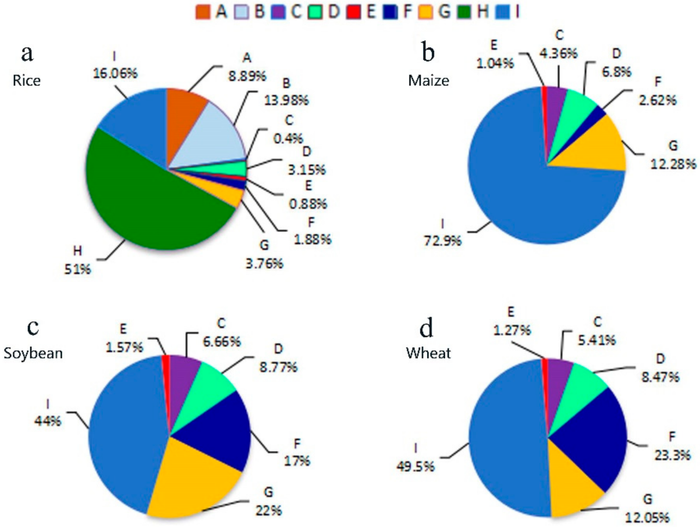
Agricultural material inputs or sources to the HLRA CF are shown in Figure 5. For rice production, 51% of the CF was derived from CH₄ emissions, followed by the sum of direct N₂O emissions and indirect emissions from N fertilizer use (16.06%), electricity for irrigation (13.98%) and plastic film (8.89%). The remaining five inputs and farming operations amounted to 10.07% of the total CF.

In contrast, the sum of direct N₂O emissions and indirect emissions from N fertilizer use was the largest contributor to the CFs of dry crops (maize, soybeans, and wheat), accounting for 72.9%, 44%, and 49.5% of the CF for maize, soybean, and wheat production, respectively. The second largest contributor to the total CFs for both maize and soybean production was diesel (12.28% and 22%, respectively), and seed was the second largest contributor for wheat production (23.3%), followed by diesel (12.05%). Overall, N fertilizer input and N₂O from N fertilizer use were the dominant sources of GHG emissions in dry crop production, although CH₄ was the dominant source of GHG emissions in rice production. In contrast, pesticides contributed a small amount to each crop’s CF, especially for rice production (0.4%).

4.3. Analysis of the CF of Rice Production

As reported above, rice production played an important role in the HLRA and constituted the vast majority of the CF in this region (80%). In recent decades, eight branches (except the SH branch) experienced a weak decoupling between crop production and GHG emissions (Table 6). Here, we take the JSJ branch and the SH branch of the HLRA for comparative analysis (Figure 6 and Figure 7).

The JSJ branch is the largest branch in the HLRA, and its rice planting area and rice yield occupied 41% and 43% of the HLRA total. In contrast, the rice planting area and rice yield in the SH branch each occupied 2% of the HLRA total. There was a distinct difference in trends between CF and rice yield between these two branches (Figure 6). According to Equation (8) for carbon intensity per area, the CF_A of rice production in the JSJ branch fluctuated from 2539 kgCEha⁻¹ to 2775 kgCEha⁻¹, which was below the average CF_A in the HLRA (2919 kgCEha⁻¹), whereas the CF_A of rice production in the SH branch fluctuated from 3323 kgCEha⁻¹ to 4503 kgCEha⁻¹.

The SH branch required more electricity for irrigation, more fertilizer input (especially more N fertilizer), and more diesel input per unit area, all of which contributed to a higher CF_A for rice production (Figure 7). It is clear that high material inputs with low utilization efficiency contributed to its degree of expansive coupling. Based on this result, we suggest targeted measures for the SH branch to mitigate GHG emissions from rice production, such as decreasing agricultural material inputs (including fertilizers, electricity for irrigation, diesel, and plastic films), improving the utilization efficiency of agricultural material inputs and increasing agricultural productivity.

5. Conclusions

In this paper, a decoupling index based on carbon footprint and crop yield was used to examine the relationship between crop production and GHG emissions in the HLRA during the years 2001–2015. The results indicated that various decoupling degrees (including strong decoupling, weak decoupling, and recessive decoupling) occurred during more than half of the study phase across the entire HLRA, although each branch showed weak decoupling based on the average value from 2001 to 2015. In addition, rice production constituted 80% of the total CF in the HLRA, and weak decoupling occurred more frequently at the scale of the entire study area and at the branch scale (except for the SH branch, which showed expansive coupling).

Seen from the results of the decoupling analysis, although a high appearance frequency of weak decoupling occurred during 2001–2015 in the HLRA, the status of weak decoupling was not steady, which highlights both pressures and challenges for the HLRA as it develops towards green growth. We also found that high material inputs with low utilization efficiency contributed to a poor relationship between crop production and GHG emissions and that fertilizer was an important contributor to the total CF of crop production. Since it is the major source of GHG emissions from agriculture in the HLRA, we should pay more attention to rice production, in particular for the SH branch.

The current work of decoupling analysis aims to examine the relationship between GHG emissions and crop production, using HLRA as an example. In fact, there is a limitation to the decoupling concept, which lacks a direct contact with the environmental process. Based on the results of decoupling analysis, next we will borrow from the experience of others and use the LMDI decomposition methodology to analyze factors that affect GHG emissions in crop production processes, in view of the activity effect, the structure effect, and the intensity effect. Further integrating more detailed information about GHG emissions from crop production processes could contribute to more targeted suggestions for low-carbon agriculture.

References

- Arrow, K.; Bolin, B.; Costanza, R.; Dasgupta, P.; Folke, C.; Holling, C.S.; Jansson, B.O.; Levin, S.; Maler, K.G.; Perrings, C.; et al. Economic Growth, Carrying Capacity and the Environment. Science 1995, 268, 520–521. [Google Scholar] [CrossRef] [PubMed]
- Holdren, J.P. Science and Technology for Sustainable Well-being. Science 2008, 319, 424–434. [Google Scholar] [CrossRef]
- Magazzino, C. The Relationship among Economic Growth, CO2 Emissions and Energy Use in the APEC Countries: A Panel VAR Approach. Environ. Syst. Decis. 2017, 37, 353–366. [Google Scholar] [CrossRef]
- United Nations Environment Programme. Options for Decoupling Economic Growth from Water Use and Water Pollution; Report of the International Resource Panel Working Group on Sustainable Water Management; UNEP: Nairobi, Kenya, 2015; pp. 1–73. [Google Scholar]
- United Nations Environment Programme. Decoupling 2: Technologies, Opportunities and Policy Options; A Report of the Working Group on Decoupling to the International Resource Panel; UNEP: Nairobi, Kenya, 2014; pp. 1–158. [Google Scholar]
- Grossman, G.M.; Krueger, A.B. Economic Growth and the Environment. Q. J. Econ. 1995, 110, 353–377. [Google Scholar] [CrossRef]
- Organisation for Economic Co-operation and Development. Indicators to Measure Decoupling of Environmental Pressure from Economic Growth; OECD: Paris, France, 2002; pp. 1–3. [Google Scholar]
- Tapio, P. Towards a Theory of Decoupling: Degrees of Decoupling in the EU and the Case of Road Traffic in Finland between 1970 and 2001. J. Transp. Policy 2005, 12, 137–151. [Google Scholar] [CrossRef]
- Diakoulaki, D.; Mandaraka, M. Decomposition Analysis for Assessing the Progress in Decoupling Industrial Growth from CO2 Emissions in the EU Manufacturing Sector. Energy Econ. 2007, 29, 636–664. [Google Scholar] [CrossRef]
- Roman, R.; Cansino, J.M.; Botia, C. How far is Colombia from Decoupling? Two-level decomposition analysis of energy consumption changes. Energy 2018, 148, 687–700. [Google Scholar] [CrossRef]
- Schandl, H.; Hatfield-Dodds, S.; Wiedmann, T.; Geschke, A.; Cai, Y.; West, J.; Newth, D.; Baynes, T.; Lenzen, M.; Owen, A. Decoupling Global Environmental Pressure and Economic Growth: Scenarios for Energy Use, Materials Use and Carbon Emissions. J. Clean. Prod. 2016, 132, 45–56. [Google Scholar] [CrossRef]
- Roman, R.; Cansino, J.M.; Rodas, J.A. Analysis of the Main Drivers of CO2 Emissions Changes in Colombia (1990–2012) and its Political Implications. Renew. Energy 2018, 116, 402–411. [Google Scholar] [CrossRef]
- United Nations Environment Programme. Decoupling Natural Resource Use and Environmental Impacts from Economic Growth; A Report of the Working Group on Decoupling to the International Resource Panel; UNEP: Nairobi, Kenya, 2011; pp. 1–174. [Google Scholar]
- Intergovernmental Panel on Climate Change. Climate change 2007: The Physical Science Basis. In Contribution of the Working Group I to the Fourth Assessment Report of the Intergovernmental Panel on Climate Change; Cambridge University Press: Cambridge, UK; New York, NY, USA, 2007; Available online: http://www.ipcc.ch/ pdf/assessment-report/ar4/syr/ar4_syr.pdf (accessed on 6 June 2018).
- Intergovernmental Panel on Climate Change. Climate Change 2013: The Physical Science Basis. In Contribution of Working Group I to the Fifth Assessment Report of the Intergovernmental Panel on Climate Change; Cambridge University Press: Cambridge, UK; New York, NY, USA, 2013; pp. 1–1535. [Google Scholar]
- Perry, S.; Klemes, J.; Bulatov, I. Integrating Waste and Renewable Energy to Reduce the Carbon Footprint of Locally Integrated Energy Sectors. Energy 2008, 33, 1489–1497. [Google Scholar] [CrossRef]
- Hillier, J.; Hawes, C.; Squire, G.; Hilton, A.; Wale, S.; Smith, P. The Carbon Footprints of Food Crop Production. Int. J. Agric. Sustain. 2009, 7, 107–118. [Google Scholar] [CrossRef]
- Liu, Y.; Xiao, H.W.; Zikhali, P.; Lv, Y.K. Carbon Emissions in China: A Spatial Econometric Analysis at the Regional Level. Sustainability 2014, 6, 6005–6023. [Google Scholar] [CrossRef] [Green Version]
- Smith, P.; Martino, D.; Cai, Z.C.; Gwary, D.; Janzen, H.; Kumar, P.; McCarl, B.; Ogle, S.; O’Mara, F.; Rice, C.; et al. Greenhouse Gas Mitigation in Agriculture. Philos. Trans. Biol. Sci. 2008, 363, 789–813. [Google Scholar] [CrossRef] [PubMed]
- McDougall, F.; White, P.; Franke, M.; Hindle, P. Integrated Solid Waste Management: A Life Cycle Inventory; Blackwell Science: London, UK, 2001. [Google Scholar]
- Lal, R. Carbon Emission from Farm Operations. Environ. Int. 2004, 30, 981–990. [Google Scholar] [CrossRef] [PubMed]
- Ponsioen, T.C.; Blonk, T.J. Calculating Land Use Change in Carbon Footprints of Agricultural Products as an Impact of Current Land Use. J. Clean. Prod. 2012, 28, 120–126. [Google Scholar] [CrossRef]
- Clair, S.S.; Hiller, J.; Smith, P. Estimating the pre-harvest greenhouse gas costs of energy crop production. Biomass Bioenergy 2008, 32, 442–452. [Google Scholar] [CrossRef]
- Knudsen, M.T.; Meyer-Aurich, A.; Olesen, J.E.; Chirinda, N.; Hermansen, J.E. Carbon footprints of crops from organic and conventional arable crop rotations—Using a life cycle assessment approach. J. Clean. Prod. 2014, 64, 609–618. [Google Scholar] [CrossRef]
- Yan, M.; Cheng, K.; Luo, T.; Yan, Y.; Pan, G.; Robert, M.R. Carbon footprint of grain crop production in china-based on farm survey data. J. Clean. Prod. 2015, 104, 130–138. [Google Scholar] [CrossRef]
- Huang, X.; Chen, C.; Chen, M.; Song, Z.; Deng, A.; Zhang, J.; Zheng, C.; Zhang, W. Carbon Footprints of Major Staple Grain Crops Production in Three Provinces of Northeast China during 2004–2013. Chin. J. Appl. Ecol. 2016, 27, 3307–3315. [Google Scholar]
- Dubey, A.; Lal, R. Carbon Footprint and Sustainability of Agricultural Production Systems in Punjab, India, and Ohio, USA. J. Crop Improv. 2009, 23, 332–350. [Google Scholar] [CrossRef]
- Cheng, K.; Yan, M.; Nayak, D.; Smith, P.; Pan, G.; Zheng, J. Carbon Footprint of Crop Production in China: An Analysis of National Statistics Data. Sci. Agric. Sin. 2015, 153, 422–431. [Google Scholar] [CrossRef]
- Xue, J.; Pu, C.; Liu, S.; Zhao, X.; Zhang, R.; Chen, F.; Xiao, X.; Zhang, H. Carbon and Nitrogen Footprint of Double Rice Production in Southern China. Ecol. Indic. 2016, 64, 249–257. [Google Scholar] [CrossRef]
- Wang, X.; Zhao, X.; Wang, Y.; Xue, J.; Zhang, H. Assessment of the Carbon Footprint of Rice Production in China. Resour. Sci. 2017, 39, 713–722. [Google Scholar]
- Huang, Y.; Zhang, W.; Zheng, X.; Han, S.; Yu, Y. Estimates of Methane Emission from Chinese Paddy Fields by Linking A Model to GIS Database. Acta Ecol. Sin. 2006, 6, 980–988. [Google Scholar] [CrossRef]
- Gan, Y.; Liang, B.; May, W.; Malhi, S.S.; Niu, J.; Wang, X. Carbon Footprint of Spring Barley in Relation to Preceding Oilseeds and N Fertilization. Int. J. Life Cycle Assess. 2012, 17, 635–645. [Google Scholar] [CrossRef]
- Wang, Y.; Zhao, X.; Li, K.; Wang, X.; Xue, J.; Zhang, H. Dynamics of Carbon Footprint for Wheat Production in the North China Plain. China Popul. Resour. Environ. 2015, S2, 258–261. [Google Scholar]
- Dyer, J.A.; Kulshreshtha, S.N.; McConkey, B.G.; Desjardins, R.L. An assessment of fossil fuel energy use and CO2 emissions from farm field operations using a regional level crop and land use database for Canada. Energy 2010, 35, 2261–2269. [Google Scholar] [CrossRef]
- Koga, N.; Tsuruta, H.; Tsuji, H.; Nakano, H. Fuel Consumption-derived CO2 Emissions under Conventional and Reduced Tillage Cropping Systems in Northern Japan. Agric. Ecosyst. Environ. 2003, 99, 213–219. [Google Scholar] [CrossRef]
- Tian, Y.; Zhang, J.; Li, B. Intensities of Agricultural Carbon Emissions and Their Causes in the Major Grain Producing Areas in China. Prog. Geogr. 2012, 31, 1546–1551. [Google Scholar]
- Cheng, K.; Pan, G.; Smith, P.; Luo, T.; Li, L.; Zheng, J.; Zhang, X.; Han, X.; Yan, M. Carbon Footprint of China’s Crop Production–An Estimation Using Agro-statistics Data over 1993–2007. Agric. Ecosyst. Environ. 2011, 142, 231–237. [Google Scholar] [CrossRef]
- Yang, Q.; Liu, J.; Zhang, Y. Decoupling Agricultural Nonpoint Source Pollution from Crop Production: A Case Study of Heilongjiang Land Reclamation Area, China. Sustainability 2017, 9, 1024. [Google Scholar] [CrossRef]
- Zou, J.; Huang, Y.; Zheng, X.; Wang, Y. Quantifying Direct N2O Emissions in Paddy Fields during Rice Growing Season in Mainland China: Dependence on Water Regime. Atmos. Environ. 2007, 41, 8030–8042. [Google Scholar] [CrossRef]
- Intergovernmental Panel on Climate Change. 2006 IPCC Guidelines for National Greenhouse Gas Inventories; Institute for Global Environmental Strategy: Kanagawa, Japan, 2006. [Google Scholar]
- Yan, X.; Yagi, K.; Akiyama, H.; Akimoto, H. Statistical Analysis of the Major Variables Controlling Methane Emission from Rice Fields. Glob. Chang. Biol. 2005, 11, 1131–1141. [Google Scholar] [CrossRef]
- Magazzino, C. A Panel VAR Approach of the Relationship among Economic Growth, CO2 Emissions and Energy Use in the ASEAN-6 Countries. Int. J. Energy Econ. Policy 2014, 4, 546–553. [Google Scholar]
- Jeong, K.; Kim, S. LMDI Decomposition Analysis of Greenhouse Gas Emissions in the Korean Manufacturing Sector. Energy Policy 2013, 62, 1245–1253. [Google Scholar] [CrossRef]
- Ren, S.; Yin, H.; Chen, X. Using LMDI to Analyze the Decoupling of Carbon Dioxide Emissions by China’s Manufacturing Industry. Environ. Dev. 2014, 9, 61–75. [Google Scholar] [CrossRef]
- Timilsina, G.R.; Shrestha, A. Factors Affecting Transport Sector CO2 Emissions Growth in Latin American and Caribbean Countries: An LMDI Decomposition Analysis. Int. J. Energy Res. 2009, 33, 396–414. [Google Scholar] [CrossRef]
- Wang, X. Changes in CO2 Emissions Induced by Agricultural Inputs in China over 1991–2014. Sustainability 2016, 8, 414. [Google Scholar] [CrossRef]
- Snyder, C.S.; Bruulsema, T.W.; Jensen, T.L.; Fixen, P.E. Review of Greenhouse Gas Emissions from Crop Production Systems and Fertilizer Management Effects. Agric. Ecosyst. Environ. 2009, 133, 247–266. [Google Scholar] [CrossRef]
- Gan, Y.; Liang, C.; Wang, X.; McConkey, B. Lowering Carbon Footprint of Durum Wheat by Diversifying Cropping Systems. Field Crops Res. 2011, 122, 199–206. [Google Scholar] [CrossRef]
- Pathak, H.; Jain, N.; Bhatia, A.; Patel, J.; Aggarwal, P.K. Carbon Footprints of Indian Food Items. Agric. Ecosyst. Environ. 2010, 139, 66–73. [Google Scholar] [CrossRef]
Figure 1.
Steps in the decoupling analysis.
Figure 2.
Location of the study area.
Figure 3.
Relationship between carbon footprint and crop yield in the HLRA (2001–2015).
Figure 4.
Composition of CFs for crop production in the HLRA (2001–2015). A: Plastic film; B: Electricity; C: Pesticide; D: P fertilizer; E: K fertilizer; F: Seed; G: Diesel; H: CH4; I: N fertilizer + N2O.
Figure 5.
Composition of CFs based on crop structure in the HLRA. (Average of the years 2001–2015). A: Plastic film; B: Electricity; C: Pesticide; D: P fertilizer; E: K fertilizer; F: Seed; G: Diesel; H: CH4; I: N fertilizer + N2O.
Figure 6.
Carbon intensity in area for rice production in the JSJ branch and the SH branch (2001–2015).
Figure 7.
Carbon intensity per area for rice production in the JSJ branch and the SH branch (average of the years 2001–2015).