Recurrent Neural Network for Partial Discharge Diagnosis in Gas-Insulated Switchgear


1
Department of Electronic Engineering, Myongji University, Yongin 449-728, Korea
2
Prevention Diagnosis Team, Genad System, Naju 58296, Korea
*
Author to whom correspondence should be addressed.
Energies 2018, 11(5), 1202; https://doi.org/10.3390/en11051202
Submission received: 10 April 2018
/
Revised: 29 April 2018
/
Accepted: 3 May 2018
/
Published: 9 May 2018
(This article belongs to the Section F: Electrical Engineering)
Abstract
:The analysis of partial discharge (PD) signals has been identified as a standard diagnostic tool for monitoring the condition of different electrical apparatuses. This study proposes an approach to detecting PD patterns in gas-insulated switchgear (GIS) using a long short-term memory (LSTM) recurrent neural network (RNN). The proposed method uses phase-resolved PD (PRPD) signals as input, extracts low-level features, and finally, classifies faults in GIS. In the proposed method, LSTM networks can learn temporal dependencies directly from PRPD signals. Most existing models use support vector machines (SVMs) and mainly focus on improving feature representation and extraction manually to analyze PRPD signals. However, the proposed model captures important temporal features with the help of its low-level feature extraction capability from raw inputs. It outperforms conventional SVMs and achieves 96.74% classification accuracy for PRPDs in GIS.
1. Introduction
Power systems are rapidly growing in popularity because of increasing power demands, and the reliability of the power grid is critical to stable power system operation. The gas-insulated switchgear (GIS), which is applied to a substation, is the main protection device for electric power facilities. It is a device that protects the electric power system by not only opening and closing normally, but also by quickly shutting off excessive current in case of a fault. In the case of a GIS, if a failure occurs and overcurrent happens, it will cause large-scale effects and requires a long time to recover from the accident. In addition, the power failure time becomes lengthy. Various abnormalities that cause dielectric breakdown of GISs also cause partial discharge before dielectric breakdown. Therefore, detecting partial discharges (PDs) in GISs to avoid failures and ensure high reliability and safety is crucial [1,2,3,4,5,6]. Various electrical, mechanical, and chemical methods have been used to detect PDs in GISs [7,8]. Some existing electrical methods use ultra-high frequency (UHF) sensors [9,10,11,12,13], while sound measurement methods use acoustic sensors [14,15] and chemical methods use dissolved gas analysis [16,17]. In this study, an electrical method that employs a UHF sensor is used for the PD measurement system.
Time-resolved PD (TRPD) and phase-resolved PD (PRPD) analyses have been studied in order to examine the characteristics of PDs in GIS [18,19,20,21,22,23,24,25,26,27]. The TRPD-based method is a method of analyzing the time-domain features of PD pulses, frequency-domain features of PD pulses, and both time-domain and frequency-domain features of PD pulses [19,20,21]. The PRPD-based diagnostic method analyzes phase-amplitude-number (--) measurements, where is the phase angle, is the amplitude, and n is the number of discharges [26]. It identifies the fault type by analyzing the number of PD pulses, the maximum amplitude, or the average amplitude in each phase [19,20,21,25,27,28]. From these features, fault types are classified by many methods, including a knowledge-based fuzzy logic analysis [26] and machine learning techniques such as K-means cluster analysis [23,29], artificial neural networks (ANNs) [19,27,30,31], or support vector machines (SVMs) [19,20,21,25,32,33]. Among the ANN and fuzzy logic methods, ANNs provide higher accuracy in classifying fault types and fault severities [26]. However, existing methods have studied either feature extraction or classification for PD diagnosis. To improve the accuracy of fault diagnosis, it is necessary to consider feature extraction from raw data and classification simultaneously.
In this study, a data-based approach to PRPD diagnosis that combines automatic feature extraction and PRPD classification is proposed. The proposed method is based on a recurrent neural network (RNN) chosen from a variety of deep neural networks that have recently achieved state-of-the-art performances in a range of pattern recognition tasks [34]. The RNN model has been actively applied to various fields, such as language modeling [35], speech recognition [36], and machine translation [37]. When compared to traditional neural network structures, such as those of a fully-connected neural network and a convolutional neural network, an RNN model uses a recurrence formula during every time step in order to consider sequential information [35]. This makes it a candidate to model PRPD patterns. The long short-term memory (LSTM) model, which is one of the most widely used RNN models, avoids the long-term dependency problem caused by the vanishing gradient in gradient-based learning methods by using four gates to adjust the flow of information [38]. For LSTM models, we use experimental PRPDs with training data to determine appropriate parameters for the model. The trained network is analyzed using t-distributed stochastic neighbor embedding (t-SNE) for the visualization of high-dimensional datasets [39]. The following contributions are made in this study:
- For the first time, an RNN structure is applied to classify PRPDs in a GIS. The proposed LSTM RNN model can learn features from PRPDs without manual feature extraction.
- To obtain training and test data for the proposed LSTM RNN model, we conduct PRPD and noise experiments for a GIS. We collect extensive data with respect to various fault types and noise for a GIS.
- The performance of the proposed LSTM RNN model is verified with conventional ANNs and SVMs. The proposed method yields highly accurate results even for the PRPD data observed in a very short time. Therefore, it considerably reduces the number of PRPDs for PD classification, thus saving the data for fault diagnosis.
2. Experiments in the GIS
In this section, we present our experimental setup and results obtained from PRPD measurements after modeling four types of artificial defects—namely protruding electrodes, floating electrodes, free particles, and void defects. In addition, we conducted artificial noise measurements to obtain data for noise.
2.1. PRPDs in the GIS
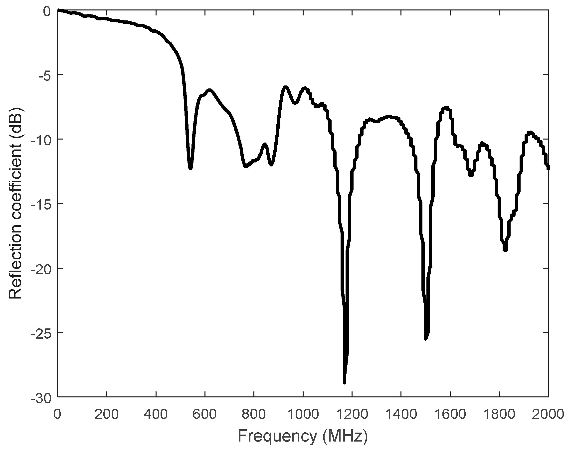
In the measurement system, artificial cells for the modeling of PDs and an external UHF sensor were installed in the 345 kV GIS chamber. Figure 1 shows the measurement system for conducting PRPD experiments in the GIS. A high voltage was applied to the AC voltage tester to generate the GIS PD signal in one of our experiments. The cavity-backed patch antenna for the external UHF sensor and an amplifier with a gain of 45 dB and a signal bandwidth ranging from 500 MHz to 1.5 GHz were used for PD detection. Figure 2 shows the measured reflection coefficient of the external UHF sensor using an E5071C network analyzer. The measured reflection coefficient was less than −6 dB in the target frequency range from 500 MHz to 1.5 GHz, which allowed the external UHF sensor to operate with a favorable impedance matching.
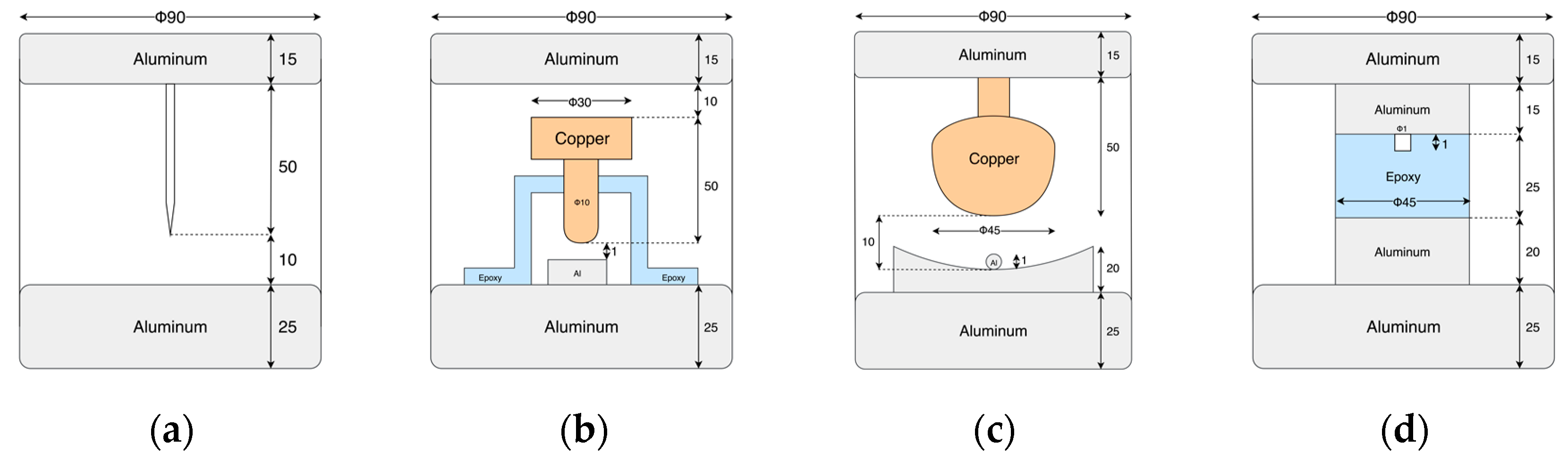
Figure 3 displays the artificial cells that model four types of faults (corona, floating, particle, and void PDs) to simulate possible defects in a GIS. As shown in Figure 3a, the artificial cell for modeling the corona simulated the protrusion of an electrode through a needle with a tip radius of 10 μm and a diameter of 1 mm (Ogura), while the distance between the needle and the ground electrode was 10 mm, and the test voltage was 11 kV. To simulate an unconnected cell, the cell of a floating electrode was fabricated with 10 mm between the high-voltage (HV) and middle electrodes, and 1 mm between the middle and ground electrodes, as illustrated in Figure 3b, where the test voltage was 10 kV. To simulate the free particle discharge, a small sphere with a diameter of 1.0 mm was placed on a concave ground electrode, and the HV electrode was a 45-mm-diameter sphere fixed at 10 mm from the ground electrode, where the test voltage was 10 kV, as represented in Figure 3c. For the artificial void defect, there was a small gap between the epoxy disc and the upper electrode, as shown in Figure 3d, where the test voltage was 8 kV. All artificial cells were filled with 0.2 MPa of sulfur hexafluoride (SF6) gas.
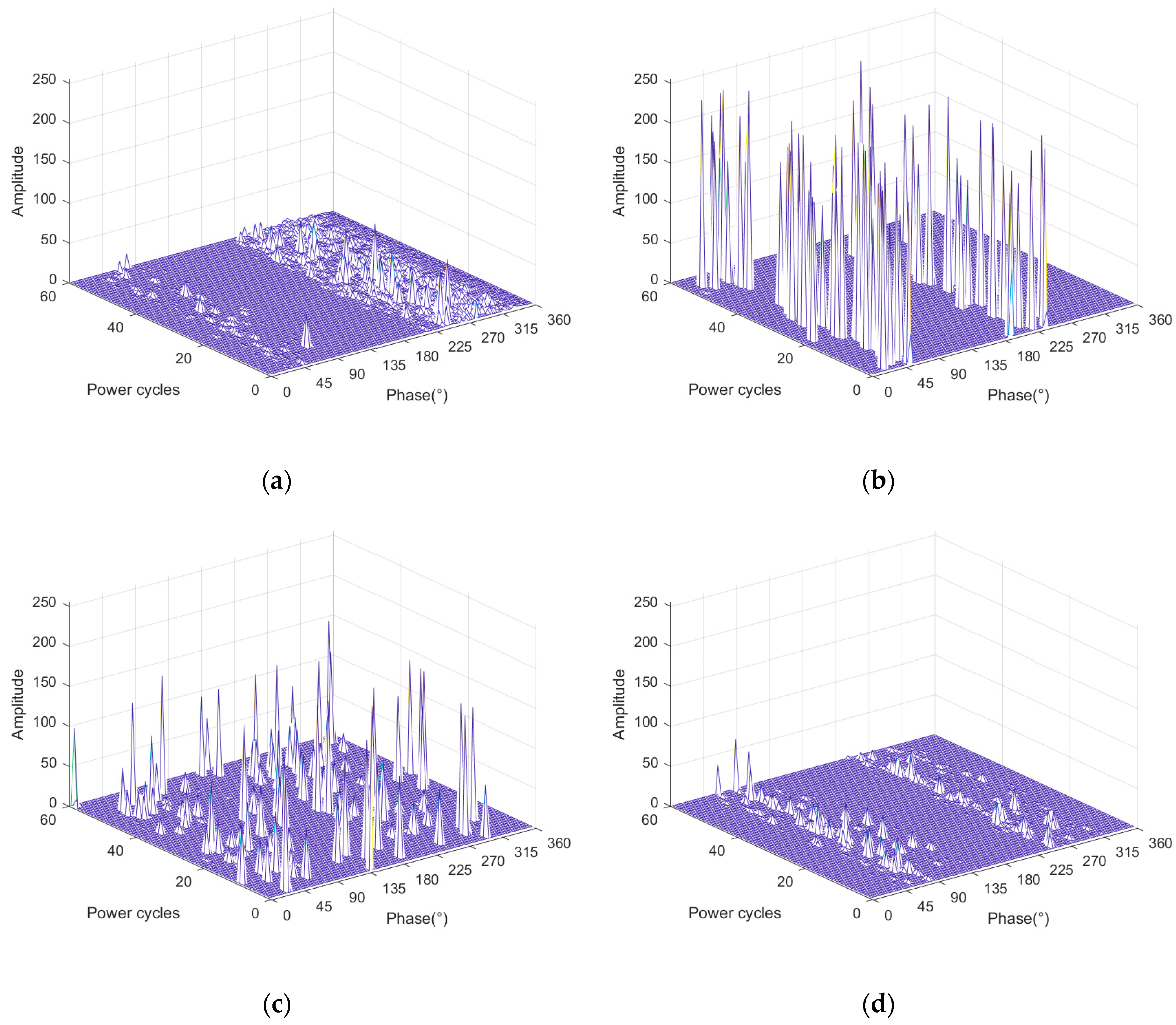
Figure 4 presents the PRPDs, with 60 power cycles in the four artificial cells, recorded through the UHF sensor. In the PRPDs recorded by the UHF sensor, the 360° power cycle was divided into small-phased windows. Some corona PDs were observed in the positive half-cycle band (from 0° to 180°), but they were more densely distributed in the negative half-cycle band (from 180° to 360°), as shown in Figure 4a. The floating PDs were clearly observed in the positive and negative half cycles, as depicted in Figure 4b. The particle PDs were distributed across all bands, as depicted in Figure 4c. Figure 4d shows that the void PDs were observed around 90° and 270°.
2.2. Noise Measurement
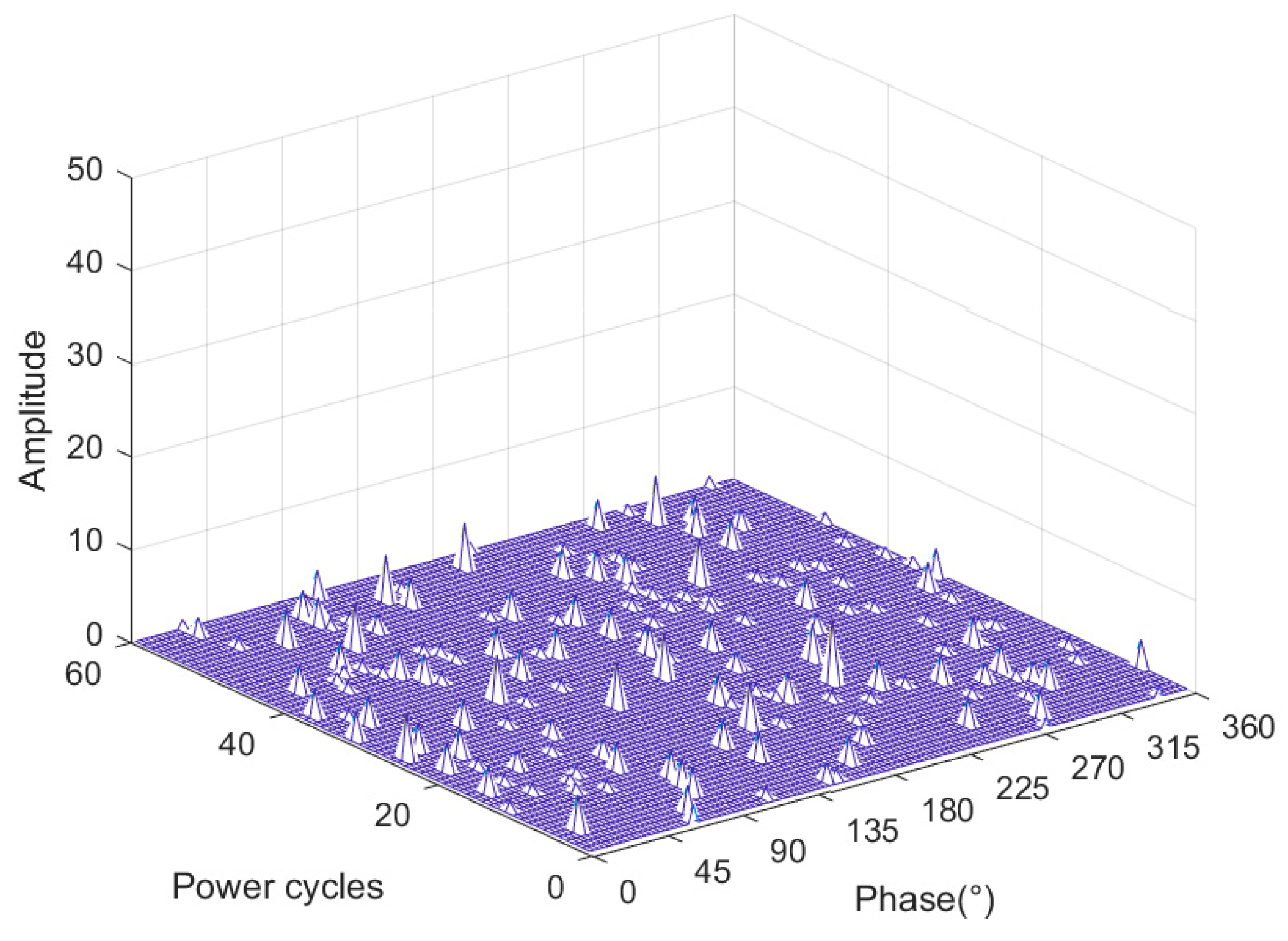
Noise measurements were performed by generating artificial noises that might occur in power grids. In the noise measurements, an air purifier (Samsung AC-121B) was used as a noise source and noise signals were obtained using the external UHF sensor. One example of noise signals is shown in Figure 5. Here, noise signals exist in all ranges of phases and power cycles, and the amplitudes of noise signals are smaller than those of PRPDs in the GIS.
3. Neural Network Model for Diagnosing PRPDs
In this section, we propose an LSTM RNN model to detect PRPDs in the GIS. The first task was to generate an appropriate input vector from the PRPD measurements. The PRPD signal at the m-th power cycle was defined as:
where and was the number of data points in a power cycle.
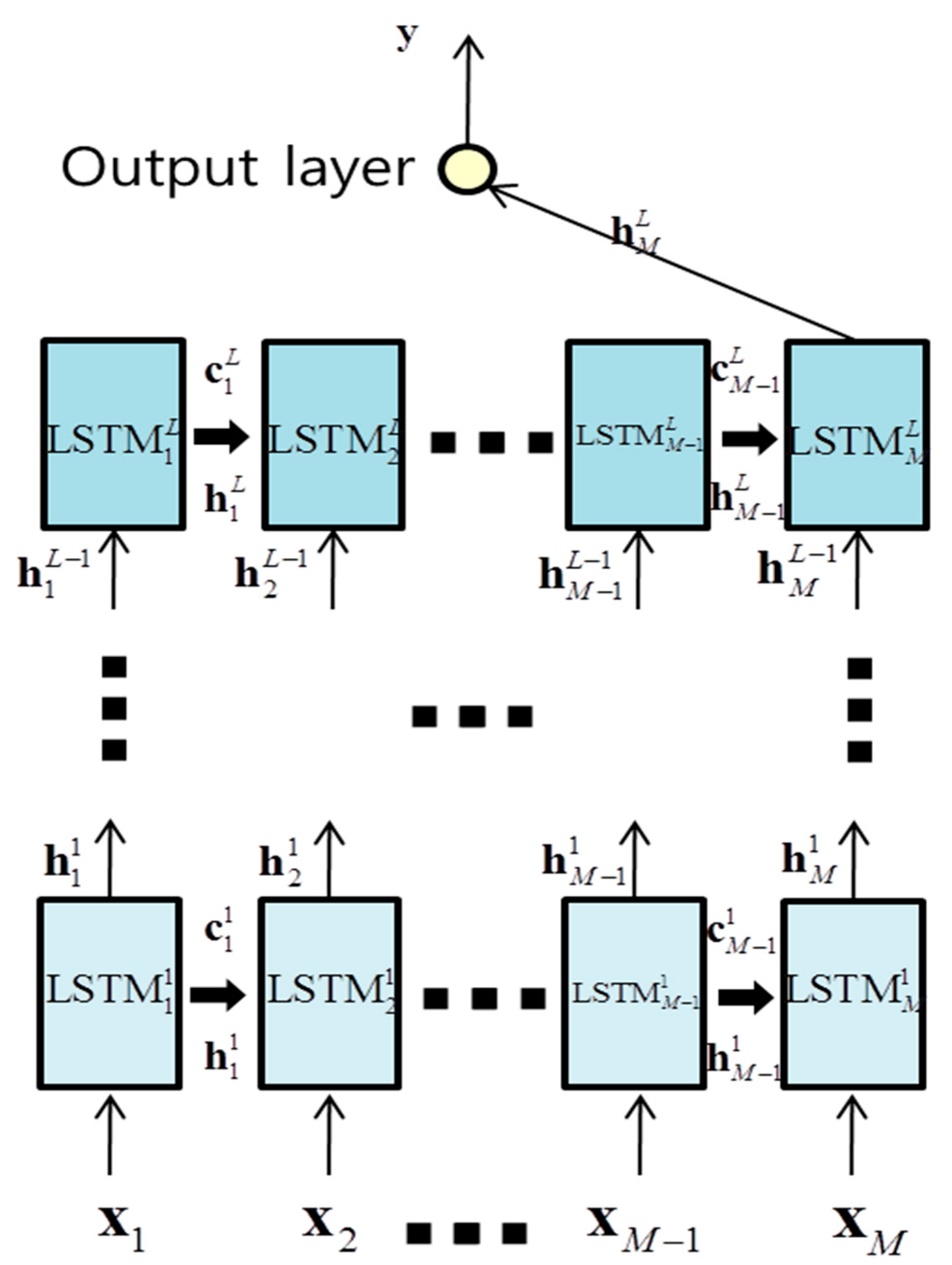
Figure 6 shows the architecture of the proposed RNN model, which was composed of LSTM modules and an output layer for classification. The standard RNN structure causes the gradient descent method in the network to struggle in minimizing the cost function because of a vanishing gradient, which means long-term dependencies become exponentially smaller in the sequence and therefore have less impact on the gradient when compared to short-term dependencies. Among many LSTM-based structures, the proposed RNN is a many-to-one model and conducts representation learning of deep learning.
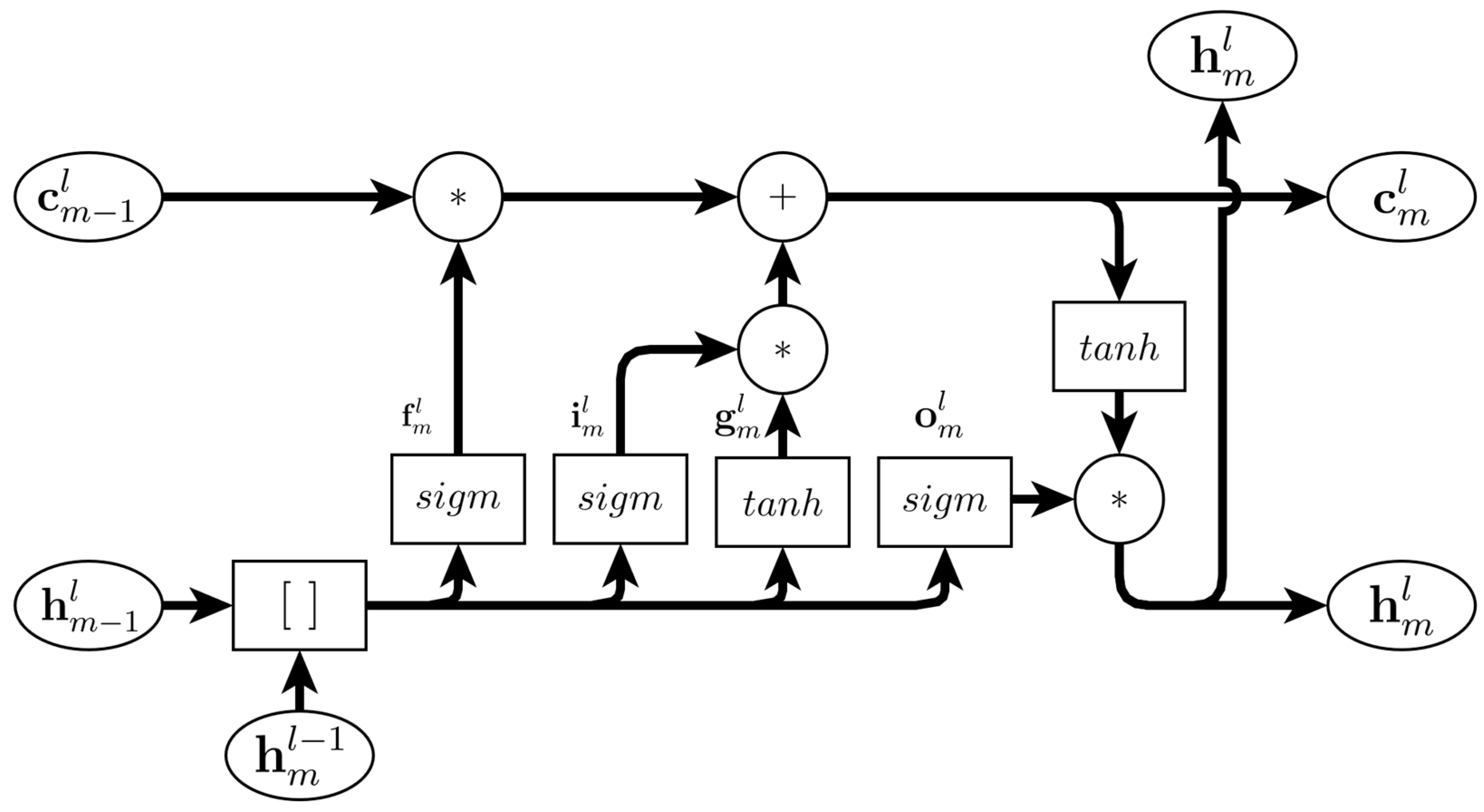
The structure of the LSTM module is shown in Figure 7. The inputs to the m-th LSTM module in layer l consisted of , , and , where was the output of the m-th LSTM module in the previous layer l − 1, and and were the outputs of the (m − 1)-th LSTM module in the current layer l. The equations below describe the internal structure of the cell at the m-th LSTM module in layer l:
where are weight matrices, are bias vectors, denotes an element-wise multiplication, is a sigmoid activation function, is a hyperbolic tangent activation function, and denotes a concatenation. For the first layer, the inputs of LSTM blocks were the PRPD vectors as , where . The LSTM model avoids long-term dependency obstacles by using four hidden layers as four gates to adjust the flow of information [38], where each gate controlled the information flow in cell state .
- -
- is the forget gate, which can decide what information is unnecessary from the cell state.
- -
- is the input gate, which decides which values in the cell state should be updated.
- -
- is the external output gate, which is a vector of new candidate values that could be added to the state. gates are used to modify the cell state between time steps as shown in Equation (2).
- -
- is the output gate, which acts as a filter to decide what parts of the current cell state should go the output, . The cell state is then put through and filtered through to become the hidden state of the current time step as shown in Equation (3).
In the proposed model, the output y for K classes is related to the last LSTM layer z as follows:
where , is a by weight matrix, is a by bias vector, and is a softmax function. In Equation (8), the j-th element of represents the likelihood that the fault is recognized as the j-th category in K classes and is defined as:
The parameters of the proposed LSTM RNN model were learned through the training data set to minimize the following cost function:
where is the number of elements in a set and is the loss value of the g-th training data. In Equation (10), measures how accurately the proposed LSTM RNN model predicts that the label corresponds to the training data, where and for if the target classification is a fault type j. Among the many choices of loss functions, we used cross-entropy, which is expressed by:
where from Equation (9) if the target classification of the g-th training data is a type j fault.
To minimize the loss function, many variants of the gradient descent method have been examined in previous studies. These include AdaGrad, AdaDelta, and Adam optimizers [40,41,42]. These optimizers adaptively change the learning rate to minimize the loss function in a precise manner. In this study, the Adam optimization algorithm was applied with a learning rate of 0.001 to train our proposed LSTM RNN model [42]. Adam was chosen because it requires that only first-order gradients be calculated, thus reducing computational complexity.
4. Performance Evaluation
In this section, we discuss the performance evaluation results of the proposed RNN model using PRPDs in the GIS. We conducted artificial noise measurements and PD experiments for four types of faults—namely, corona, floating, particle, and void PDs. The numbers of experiments for each fault type are given in Table 1, where the PRPD signals or noise signals with power cycles were obtained in one experiment.
We divided the dataset into three parts: training, validation, and test sets. For these three sets, we used 80%, 10%, and 10% of the data, respectively. During the training process, the optimization step was carried out in small batches of 512 samples. To prevent overfitting, we applied an early stopping technique so that the training process stopped itself when the validation accuracy was stable after 10 consecutive epochs. The model was implemented using TensorFlow [43] and Keras [44].
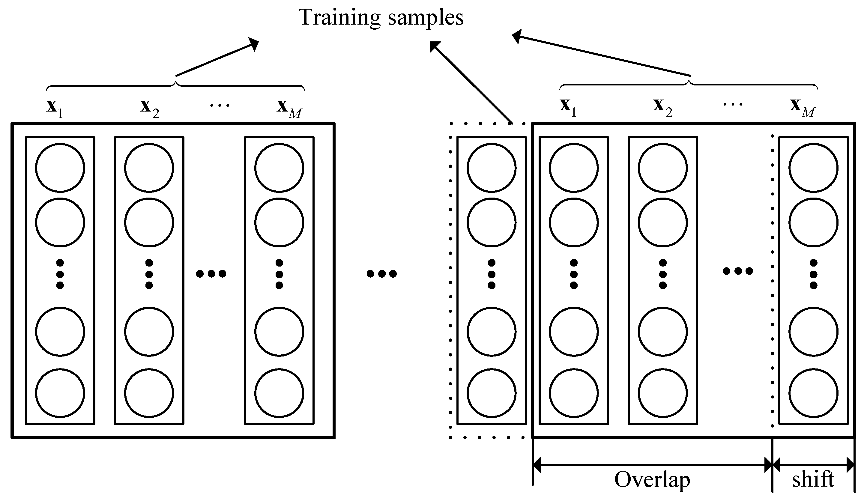
Without sufficient training samples, the deep learning model will easily run into an overfitting problem [45]. In deep learning models, data augmentation is frequently used to increase the number of training samples in order to enhance the generalization performance [45]. Here, slicing the experimental data with overlap was used to achieve high classification precision in fault diagnosis. This process is shown in Figure 8. For example, a single PRPD experiment with 3600 cycles can provide the proposed RNN with training samples, each with a length of when the shift size is 1.
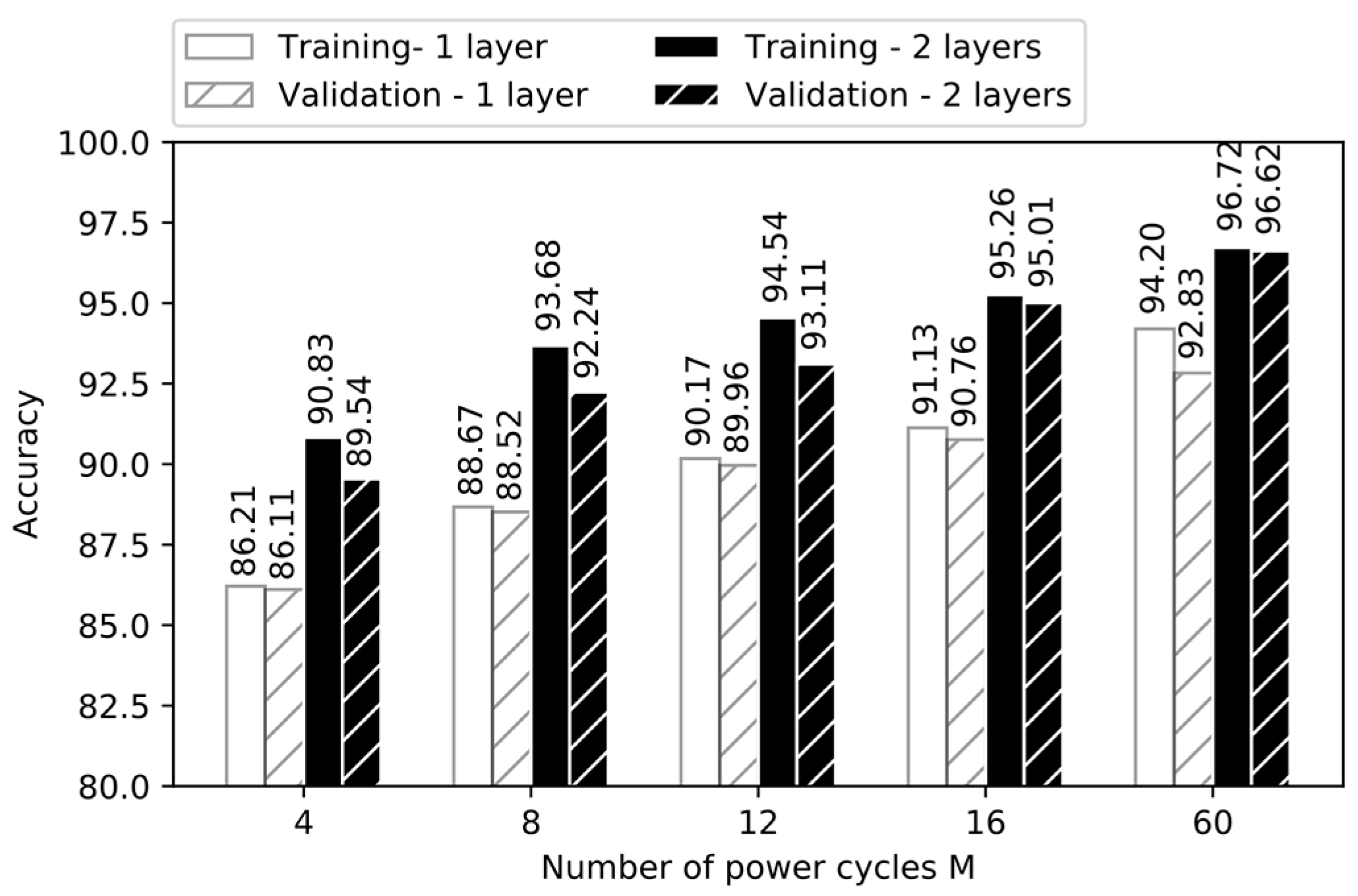
Multiple experiments with different parameters were conducted using the validation data to tune our model. Figure 9 shows the training and validation accuracies of the proposed RNN model according to the number of power cycles for or layer models. The accuracy improved as the number of power cycles increased. This was because more information about PRPDs () could be obtained as increased. In addition, when the model expanded to a larger scale, the accuracy increased because more parameters were introduced, thus better fitting the model to the data. We set the power cycles to and the number of layers to .
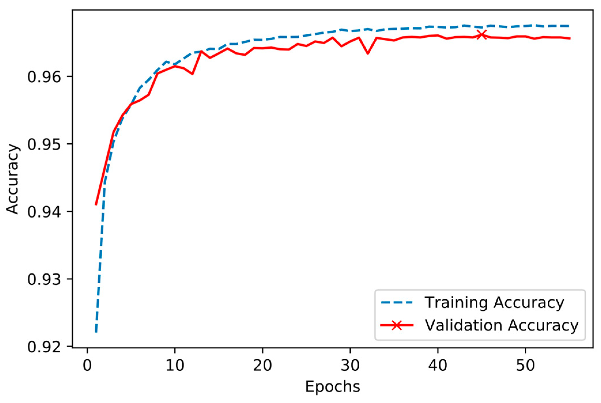
Figure 10 illustrates the convergence of the model over epochs with the training and validation set. As shown in this figure, the accuracy with training data tended to improve with the epoch, whereas the accuracy with cross-validation data diminished up to a certain epoch and then improved again. After achieving the maximum accuracy, the model firstly paused, recorded the parameters, and then continued the training process for an additional 10 epochs. This was part of the early stopping method for identifying another peak. After determining that the accuracy with cross-validation data could not be further improved, the model stopped the training process to prevent overfitting the training dataset. As the figure shows, the training process finished after 55 epochs. The maximum accuracy of 96.62% achieved at epoch 45 with the cross-validation data is presented in Figure 10 as an “⨉” mark.
For comparison, we used an ANN model and linear and nonlinear SVMs with a radial basis function (RBF) [46,47] as baseline models. The ANN model consisted of an input layer, 2 hidden layers with 256 hidden nodes at each layer, and an output layer, where the input data was PRPDs and the cross-entropy cost function and Adam optimization function were used. In SVMs, the feature vector was obtained by the mean of the amplitudes and occurrence numbers in each phase from PRPDs [32], and therefore, was a by 1 vector. The normalized feature vectors were used to optimize and train SVMs to classify faults in the GIS. The parameter for the linear SVM and the parameters and could be learned using training data, where and .
Classification performance comparisons of the proposed LSTM RNN model, SVMs, and ANN are presented in Table 2. From this table, we can see that the proposed LSTM RNN model achieved the highest overall classification accuracy performance (96.74%), when compared to the ANN and the linear and nonlinear SVMs. Note that the ANN was superior to the SVMs and the nonlinear SVM with RBF was somewhat superior to the linear SVM. This was because the proposed LSTM RNN method automatically obtained the sequential characteristics of PRPDs from the raw input, whereas the ANN used the raw input without phase information of PRPDs and the SVMs used the manually-created feature vector that combined characteristics of PRPDs. For corona faults, the performance of the proposed method was the highest at 97.04%, approximately 1.5% higher than the ANN and the SVMs. In floating fault classifications, the performance of the proposed method achieved the best result, at 79.54%. In the case of particle faults, the performance of the proposed technique was 93.18%, which was 7.84%, 27.71%, and 15.56% better than that of the ANN, the linear SVM, and the nonlinear SVM with RBF, respectively. In the case of void faults, the proposed method achieved a nearly perfect 99.94% accuracy, better than the ANN and the SVMs. For noise classification, the proposed method outperformed all other methods and achieved a 98.26% accuracy rate.
Table 3 shows training and testing timing comparisons for the ANN, the SVMs, and the proposed LSTM RNN methods, where the timing was normalized to a hypothetical 1 GHz single-core CPU to make the measurement meaningful. In our experiments, the models were trained and tested on an NVIDIA Titan X GPU with 3584 cores, each running at 1.4 GHz. It can be seen that the training and testing times of the proposed LSTM RNN model were slower than those of the ANN and the SVMs. This was because the design of the RNN required the output of the previous time step for the current time step output calculation. The test time of the proposed LSTM RNN model took longer than that of other methods, but the test time per sample of the proposed method was only 1 (s*GHz).
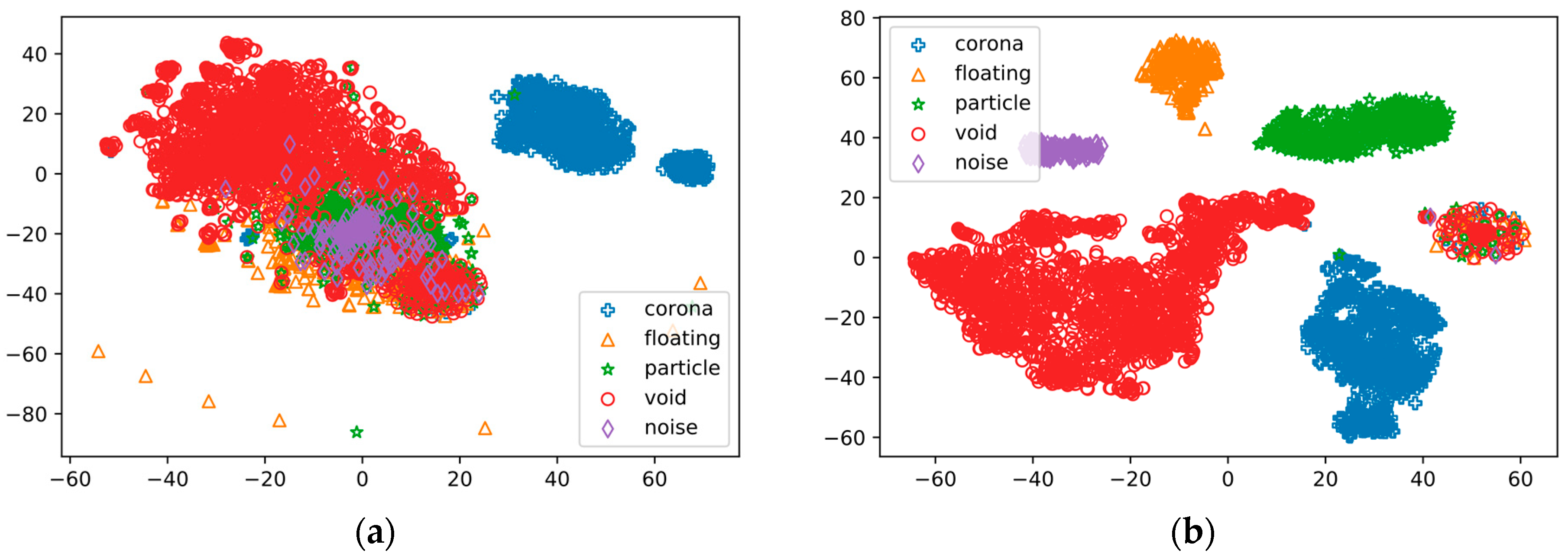
To better understand what the model learned, we analyzed the internal representations of the trained network at the end of two layers. Following the training procedure, the hidden state vectors of the last LSTM modules in the two layers were used to visualize the trained network. Figure 11 shows t-SNE representation of and using 5000 inputs from the training set, where t-SNE projected 128 dimensional vectors to two-dimensional spaces while retaining their pairwise similarity [39]. Therefore, hidden state vectors and , which are similar according to the network, occur close together in Figure 11. Here, the opposite does not have to be true because large distances in Figure 11 do not necessarily imply that the hidden state vectors and are dissimilar. In the figure, we can see that the hidden state of layer 2 was much more dispersed when compared to the hidden state of layer 1. This explains the improved accuracy based on the number of layers as shown in Figure 9. As shown in Figure 11b, the hidden states for some data of corona, floating, particle, and void faults in a GIS were similar with those for some noise data. This was because PRPDs existed with small amplitudes in the whole phase for the power cycles , as shown in Figure 4a.
5. Conclusions
Deep learning is a state-of-the-art technique used in many different applications. Using this technique, we proposed a fault diagnosis method using an LSTM RNN structure, which employed a series of PRPDs in a GIS. Instead of utilizing handcrafted features to classify PRPDs in the GIS, the proposed model efficiently learns low-level features and temporal dependencies of PRPDs using training data. To adjust parameters in the proposed model, we conducted extensive PRPD experiments using artificial defects and noise in a GIS. To lower the risk of overfitting, the data sets were obtained using data augmentation for PRPDs and were divided into three sets. These three sets were used for the purposes of training, cross-validation, and performance evaluation. The proposed model achieved a higher accuracy than the conventional ANN and SVM methods for classifying PRPDs in GIS.
The proposed method will be useful in other PRPD detections, such as power transformers and wall bushings. We hope this represents a major advancement for grid asset management and will contribute to stable power grid operation in the future.
Author Contributions
Y.-H.K. conceived of the presented idea. M.-T.N. and V.-H.N. developed the model and performed the computations. S.-J.Y. verified the experimental setup and results. All authors discussed the results and contributed to the final manuscript.
Acknowledgments
This research was supported in part by Korea Electric Power Corporation (Grant number: R17XA05-22), and in part by the Korea Institute of Energy Technology Evaluation and Planning (KETEP) and the Ministry of Trade, Industry & Energy (MOTIE) of the Republic of Korea (No. 17-02-N0202-04).
Conflicts of Interest
The authors declare no conflict of interest.
References
- Okabe, S.; Ueta, G.; Hama, H.; Ito, T.; Hikita, M.; Okubo, H. New aspects of UHF PD diagnostics on gas-insulated systems. IEEE Trans. Dielectr. Electr. Insul. 2014, 32, 2245–2258. [Google Scholar] [CrossRef]
- Wang, Y.; Wang, Z.; Li, J. UHF Moore fractal antennas for online GIS PD detection. IEEE Antennas Wirel. Propag. Lett. 2017, 16, 852–855. [Google Scholar] [CrossRef]
- Schichler, U.; Koltunowicz, W.; Gautschi, D.; Girodet, A.; Hama, H.; Juhre, K.; Lopez-Roldan, J.; Okabe, S.; Neuhold, S.; Neumann, C.; et al. UHF Partial Discharge Detection System for GIS: Application Guide for Sensitivity Verification. In Proceedings of the VDE High Voltage Technology, Berlin, Germany, 14–16 November 2016; pp. 1–9. [Google Scholar]
- Schichler, U.; Koltunowicz, W.; Endo, F.; Feser, K.; Giboulet, A.; Girodet, A.; Hama, H.; Hampton, B.; Kranz, H.-G.; Lopez-Roldan, J.; et al. Risk assessment on defects in GIS based on PD diagnostics. IEEE Trans. Dielect. Electr. Insul. 2013, 20, 2165–2172. [Google Scholar] [CrossRef]
- Kurrer, R.; Feser, K. The application of ultra-high-frequency partial discharge measurements to gas-insulated substations. IEEE Trans. Power Deliv. 1998, 13, 777–782. [Google Scholar] [CrossRef]
- Okabe, S.; Kaneko, S.; Yoshimura, M.; Muto, H.; Nishida, C.; Kamei, M. Propagation characteristics of electromagnetic waves in three-phase-type tank from viewpoint of partial discharge diagnosis on gas insulated switchgear. IEEE Trans. Dielectr. Electr. Insul. 2009, 16, 199–205. [Google Scholar] [CrossRef]
- Wu, M.; Cao, H.; Cao, J.; Nguyen, H.L.; Gomes, J.B.; Krishnaswamy, S.P. An overview of state-of-the-art partial discharge analysis techniques for condition monitoring. IEEE Trans. Electr. Insul. Mag. 2015, 31, 22–35. [Google Scholar] [CrossRef]
- Dong, M.; Zhang, C.; Ren, M.; Albarracín, R.; Ye, R. Electrochemical and Infrared Absorption Spectroscopy Detection of SF6 Decomposition Products. Sensors 2017, 17, 2627. [Google Scholar] [CrossRef] [PubMed]
- Judd, M.D.; Yang, L.; Hunter, I.B. Partial discharge monitoring of power transformers using UHF sensors. Part I: Sensors and signal interpretation. IEEE Trans. Electr. Insul. Mag. 2005, 21, 5–14. [Google Scholar] [CrossRef]
- Gao, W.; Ding, D.; Liu, W. Research on the typical partial discharge using the UHF detection method for GIS. IEEE Trans. Power Deliv. 2011, 26, 2621–2629. [Google Scholar] [CrossRef]
- Judd, M.D.; Farish, O.; Hampton, B.F. The excitation of UHF signals by partial discharges in GIS. IEEE Trans. Dielect. Electr. Insul. 1996, 3, 213–228. [Google Scholar] [CrossRef]
- Li, T.; Rong, M.; Zheng, C.; Wang, X. Development simulation and experiment study on UHF partial discharge sensor in GIS. IEEE Trans. Dielect. Electr. Insul. 2012, 19, 1421–1430. [Google Scholar] [CrossRef]
- Álvarez Gómez, F.; Albarracín-Sánchez, R.; Garnacho Vecino, F.; Granizo Arrabé, R. Diagnosis of Insulation Condition of MV Switchgears by Application of Different Partial Discharge Measuring Methods and Sensors. Sensors 2018, 18, 720. [Google Scholar] [CrossRef] [PubMed]
- Cosgrave, J.A.; Vourdas, A.; Jones, G.R.; Spencer, J.W.; Murphy, M.M.; Wilson, A. Acoustic monitoring of partial discharges in gas insulated substations using optical sensors. IEE Proc. A Sci. Meas. Technol. 1993, 140, 369–374. [Google Scholar] [CrossRef]
- Markalous, S.M.; Tenbohlen, S.; Feser, K. Detection and location of partial discharges in power transformers using acoustic and electromagnetic signals. IEEE Trans. Dielect. Electr. Insul. 2008, 15, 1070–9878. [Google Scholar] [CrossRef]
- Wang, Z.; Cotton, I.; Northcote, S. Dissolved gas analysis of alternative fluids for power transformers. IEEE Trans. Electr. Insul. Mag. 2007, 23, 5–14. [Google Scholar]
- Faiz, J.; Soleimani, M. Dissolved gas analysis evaluation in electric power transformers using conventional methods a review. IEEE Trans. Dielect. Electr. Insul. 2017, 24, 1239–1248. [Google Scholar] [CrossRef]
- Piccin, R.; Mor, A.R.; Morshuis, P.; Girodet, A.; Smit, J. Partial discharge analysis of gas insulated systems at high voltage AC and DC. IEEE Trans. Dielect. Electr. Insul. 2015, 22, 218–228. [Google Scholar] [CrossRef]
- Li, L.; Tang, J.; Liu, Y. Partial discharge recognition in gas insulated switchgear based on multi-information fusion. IEEE Trans. Dielect. Electr. Insul. 2015, 22, 1080–1087. [Google Scholar] [CrossRef]
- Zhu, M.X.; Xue, J.Y.; Zhang, J.N.; Li, Y.; Deng, J.B.; Mu, H.B.; Zhang, G.J.; Shao, X.J.; Liu, X.W. Classification and separation of partial discharge ultra-high-frequency signals in a 252 kV gas insulated substation by using cumulative energy technique. IET Sci. Meas. Technol. 2016, 10, 316–326. [Google Scholar] [CrossRef]
- Gao, W.; Zhao, D.; Ding, D.; Yao, S.; Zhao, Y.; Liu, W. Investigation of frequency characteristics of typical PD and the propagation properties in GIS. IEEE Trans. Dielect. Electr. Insul. 2015, 22, 1654–1662. [Google Scholar] [CrossRef]
- Dai, D.; Wang, X.; Long, J.; Tian, M.; Zhu, G.; Zhang, J. Feature extraction of GIS partial discharge signal based on S-transform and singular value decomposition. IET Sci. Meas. Technol. 2016, 11, 186–193. [Google Scholar] [CrossRef]
- Lin, Y.H. Using k-means clustering and parameter weighting for partial-discharge noise suppression. IEEE Trans. Power Deliv. 2011, 26, 2380–2390. [Google Scholar] [CrossRef]
- Abdel-Galil, T.K.; Sharkawy, R.M.; Salama, M.M.; Bartnikas, R. Partial discharge pattern classification using the fuzzy decision tree approach. IEEE Trans. Instrum. Meas. 2005, 54, 2258–2263. [Google Scholar] [CrossRef]
- Si, W.R.; Li, J.H.; Li, D.J.; Yang, J.G.; Li, Y.M. Investigation of a comprehensive identification method used in acoustic detection system for GIS. IEEE Trans. Dielect. Electr. Insul. 2010, 17, 721–732. [Google Scholar] [CrossRef]
- Mas’ud, A.A.; Ardila-Rey, J.A.; Albarracín, R.; Muhammad-Sukki, F.; Bani, N.A. Comparison of the Performance of Artificial Neural Networks and Fuzzy Logic for Recognizing Different Partial Discharge Sources. Energies 2017, 10, 1060. [Google Scholar] [CrossRef]
- Chang, C.S.; Jin, J.; Chang, C.; Hoshino, T.; Hanai, M.; Kobayashi, N. Separation of Corona Using Wavelet Packet Transform and Neural Network for Detection of Partial Discharge in Gas-Insulated Substations. IEEE Trans. Power Deliv. 2005, 20, 1363–1369. [Google Scholar] [CrossRef]
- Zhang, X.; Xiao, S.; Shu, N.; Tang, J.; Li, W. GIS partial discharge pattern recognition based on the chaos theory. IEEE Trans. Dielect. Electr. Insul. 2014, 21, 783–790. [Google Scholar] [CrossRef]
- Peng, X.; Zhou, C.; Hepburn, D.M.; Judd, M.D.; Siew, W.H. Application of K-Means method to pattern recognition in on-line cable partial discharge monitoring. IEEE Trans. Dielect. Electr. Insul. 2013, 20, 754–761. [Google Scholar] [CrossRef] [Green Version]
- Mas’ud, A.A.; Ardila-Rey, J.A.; Albarracín, R.; Muhammad-Sukki, F. An Ensemble-Boosting Algorithm for Classifying Partial Discharge Defects in Electrical Assets. Machines 2017, 5, 18. [Google Scholar] [CrossRef]
- Mas’ud, A.A.; Albarracín, R.; Ardila-Rey, J.A.; Muhammad-Sukki, F.; Illias, H.A.; Bani, N.A.; Munir, A.B. Artificial Neural Network Application for Partial Discharge Recognition: Survey and Future Directions. Energies 2016, 9, 574. [Google Scholar] [CrossRef]
- Kim, K.H.; Kang, M.C.; Kim, M.H.; Shin, Y.J.; Kim, Y.H. Recognition method of partial discharge based on support vector machine in gas insulated switchgear. In Proceedings of the CIGRE Asia-Oceania Regional Council Technical Meeting, Auckland, New Zealand, 10–15 September 2017. [Google Scholar]
- Robles, G.; Parrado-Hernández, E.; Ardila-Rey, J.; Martínez-Tarifa, J.M. Multiple partial discharge source discrimination with multiclass support vector machines. Expert Syst. Appl. 2016, 55, 417–428. [Google Scholar] [CrossRef]
- LeCun, Y.; Bengio, Y.; Hinton, G. Deep learning. Nature 2015, 521, 436–444. [Google Scholar] [CrossRef] [PubMed]
- Mikolov, T.; Karafiát, M.; Burget, L.; Cernocký, J.; Khudanpur, S. Recurrent neural network-based language moDeliv. In Proceedings of the 11th Annual Conference of the International Speech Communication Association, Makuhari, Chiba, Japan, 26–30 September 2010; Volume 2, p. 3. [Google Scholar]
- Graves, A.; Mohamed, A.R.; Hinton, G. Speech recognition with deep recurrent neural networks. In Proceedings of the IEEE International Conference on Acoustics, Speech and Signal Processing (ICASSP), Vancouver, BC, Canada, 26–31 May 2013; pp. 6645–6649. [Google Scholar]
- Sutskever, I.; Vinyals, O.; Le, Q.V. Sequence to sequence learning with neural networks. arXiv, 2014; arXiv:1409.3215v3. [Google Scholar]
- Hochreiter, S.; Schmidhuber, J. Long short-term memory. Neural Comput. 1997, 9, 1735–1780. [Google Scholar] [CrossRef] [PubMed]
- Maaten, L.V.D.; Hinton, G. Visualizing data using t-SNE. J. Mach. Learn. Res. 2008, 9, 2579–2605. [Google Scholar]
- Duchi, J.; Hazan, E.; Singer, Y. Adaptive subgradient methods for online learning and stochastic optimization. J. Mach. Learn. Res. 2011, 12, 2121–2159. [Google Scholar]
- Zeiler, M.D. ADADELTA: An adaptive learning rate method. arXiv, 2012; arXiv:1212.5701. [Google Scholar]
- Kingma, D.P.; Ba, J. Adam: A method for stochastic optimization. arXiv, 2014; arXiv:1412.6980. [Google Scholar]
- Abadi, M.; Agarwal, A.; Barham, P.; Brevdo, E.; Chen, Z.; Citro, C.; Corrado, G.S.; Davis, A.; Dean, J.; Devin, M. TensorFlow: Large-Scale Machine Learning on Heterogeneous Distributed Systems. arXiv, 2016; arXiv:1603.04467v2. [Google Scholar]
- Keras-Team. 2015. Available online: https://github.com/fchollet/keras (accessed on 22 October 2017).
- Cui, X.; Goel, V.; Kingsbury, B. Data augmentation for deep convolutional neural network acoustic modeling. In Proceedings of the IEEE International Conference on Acoustics, Speech and Signal Processing (ICASSP), Brisbane, Australia, 19–24 April 2015; pp. 4545–4549. [Google Scholar]
- Cortes, C.; Vapnik, V. Support-vector network. Mach. Learn. J. 1995, 20, 273–297. [Google Scholar] [CrossRef]
- Huang, H.Y.; Lin, C.J. Linear and kernel classification: When to use which. In Proceedings of the SIAM International Conference on Data Mining, Miami, FL, USA, 5–7 May 2016; pp. 216–224. [Google Scholar]
Figure 1.
Measurement system in the gas-insulated switchgear (GIS): (a) block of the measurement system, and (b) high-voltage test site. PD: partial discharge; UHF: ultra-high frequency.
Figure 1.
Measurement system in the gas-insulated switchgear (GIS): (a) block of the measurement system, and (b) high-voltage test site. PD: partial discharge; UHF: ultra-high frequency.

Figure 2.
Measured reflection coefficient of the external UHF sensor.

Figure 3.
Artificial cells for the simulated (a) corona, (b) floating, (c) particle, and (d) void PDs.
Figure 3.
Artificial cells for the simulated (a) corona, (b) floating, (c) particle, and (d) void PDs.

Figure 4.
Types of phase-resolved PDs (PRPDs) observed in the GIS: (a) corona, (b) floating, (c) particle, and (d) void.
Figure 4.
Types of phase-resolved PDs (PRPDs) observed in the GIS: (a) corona, (b) floating, (c) particle, and (d) void.

Figure 5.
Noise measurements from the air purifier.

Figure 6.
Proposed recurrent neural network (RNN) structure with the long short-term memory (LSTM) block.
Figure 6.
Proposed recurrent neural network (RNN) structure with the long short-term memory (LSTM) block.

Figure 7.
Structure of the m-th LSTM block in layer l.

Figure 8.
Structure of the m-th LSTM block in layer l.

Figure 9.
Training and validation accuracies of the proposed RNN model based on the number of power cycles for or layer models.
Figure 9.
Training and validation accuracies of the proposed RNN model based on the number of power cycles for or layer models.

Figure 10.
Accuracy improvement over epochs.

Figure 11.
t-distributed stochastic neighbor embedding (t-SNE) representation of 5000 training samples at: (a) the hidden state of layer 1, and (b) the hidden state of layer 2.
Figure 11.
t-distributed stochastic neighbor embedding (t-SNE) representation of 5000 training samples at: (a) the hidden state of layer 1, and (b) the hidden state of layer 2.


Table 1.
Experimental data set.
| Fault Types | Corona | Floating | Particle | Void | Noise |
|---|---|---|---|---|---|
| Number of experiments | 94 | 35 | 66 | 242 | 16 |
Table 2.
Classification performance comparisons. ANN: artificial neural network; RBF: radial basis function; SVM: support vector machine.
Table 2.
Classification performance comparisons. ANN: artificial neural network; RBF: radial basis function; SVM: support vector machine.
| Fault Types | Overall | Corona | Floating | Particle | Void | Noise |
|---|---|---|---|---|---|---|
| Linear SVM | 88.63% | 91.87% | 73.94% | 65.47% | 98.19% | 51.94% |
| Nonlinear SVM with RBF kernel | 90.71% | 95.28% | 67.81% | 77.62% | 98.69% | 45.53% |
| ANN | 93.01% | 95.87% | 76.27% | 85.34% | 98.12% | 65.11% |
| Proposed LSTM RNN model | 96.74% | 97.04% | 79.54% | 93.18% | 99.94% | 98.26% |
Table 3.
Training and testing time comparisons.
| Train Time (min) | Train Time (min*GHz) | Test Time on Test Set (s) | Test Time per Sample (s*GHz) | |
|---|---|---|---|---|
| Linear SVM | 5 | 26,880 | ~0.2 s | 0.013 |
| Nonlinear SVM with RBF kernel | 5.66 | 30,428 | ~0.3 s | 0.02 |
| ANN | 6.66 | 35,804 | ~6 s | 0.403 |
| Proposed LSTM RNN model | 33.33 | 179,182 | ~15 s | 1 |
© 2018 by the authors. Licensee MDPI, Basel, Switzerland. This article is an open access article distributed under the terms and conditions of the Creative Commons Attribution (CC BY) license (http://creativecommons.org/licenses/by/4.0/).
Share and Cite
MDPI and ACS Style
Nguyen, M.-T.; Nguyen, V.-H.; Yun, S.-J.; Kim, Y.-H. Recurrent Neural Network for Partial Discharge Diagnosis in Gas-Insulated Switchgear. Energies 2018, 11, 1202. https://doi.org/10.3390/en11051202
AMA Style
Nguyen M-T, Nguyen V-H, Yun S-J, Kim Y-H. Recurrent Neural Network for Partial Discharge Diagnosis in Gas-Insulated Switchgear. Energies. 2018; 11(5):1202. https://doi.org/10.3390/en11051202
Chicago/Turabian StyleNguyen, Minh-Tuan, Viet-Hung Nguyen, Suk-Jun Yun, and Yong-Hwa Kim. 2018. "Recurrent Neural Network for Partial Discharge Diagnosis in Gas-Insulated Switchgear" Energies 11, no. 5: 1202. https://doi.org/10.3390/en11051202
Note that from the first issue of 2016, this journal uses article numbers instead of page numbers. See further details here.