Big Data Analytics for Discovering Electricity Consumption Patterns in Smart Cities
by
 , , , and
Rubén Pérez-Chacón
1,† ,
,
José M. Luna-Romera
2,†,
Alicia Troncoso
1,*,
Francisco Martínez-Álvarez
1 and
José C. Riquelme
2 1
Division of Computer Science, Universidad Pablo de Olavide, ES-41013 Seville, Spain
2
Division of Computer Science, University of Sevilla, ES-41012 Seville, Spain
*
Author to whom correspondence should be addressed.
†
These authors contributed equally to this work.
Energies 2018, 11(3), 683; https://doi.org/10.3390/en11030683
Submission received: 31 January 2018
/
Revised: 5 March 2018
/
Accepted: 13 March 2018
/
Published: 18 March 2018
(This article belongs to the Special Issue Data Science and Big Data in Energy Forecasting)
Abstract
:New technologies such as sensor networks have been incorporated into the management of buildings for organizations and cities. Sensor networks have led to an exponential increase in the volume of data available in recent years, which can be used to extract consumption patterns for the purposes of energy and monetary savings. For this reason, new approaches and strategies are needed to analyze information in big data environments. This paper proposes a methodology to extract electric energy consumption patterns in big data time series, so that very valuable conclusions can be made for managers and governments. The methodology is based on the study of four clustering validity indices in their parallelized versions along with the application of a clustering technique. In particular, this work uses a voting system to choose an optimal number of clusters from the results of the indices, as well as the application of the distributed version of the k-means algorithm included in Apache Spark’s Machine Learning Library. The results, using electricity consumption for the years 2011–2017 for eight buildings of a public university, are presented and discussed. In addition, the performance of the proposed methodology is evaluated using synthetic big data, which cab represent thousands of buildings in a smart city. Finally, policies derived from the patterns discovered are proposed to optimize energy usage across the university campus.
1. Introduction
Governments in many metropolises are embracing the concept of smart cities, and are beginning to collect big datasets in order to obtain valuable information from them. This information helps governments to improve the standards of living and sustainability required for their inhabitants. In order to increase the comfort and life quality of citizens, it is necessary to reduce costs and optimize the consumption of different energy resources. This reduction in costs, for instance, could improve performance in areas such as education, health-care, transport, security, and emergency services [1]. In this regard, massive storage of data using smart grid technologies is widespread [2]. For example, the energy consumption of water or electricity in public institutions is continuously monitored. However, traditional tools and techniques for storing and extracting valuable information have become obsolete due to the high computational cost of mining gigabytes of data [3]. In this sense, the advent of new machine learning tools makes it easier to mine data, but new techniques are needed to improve the processing, management, and discovery of valuable information and knowledge for organizations [4].
Given the sudden need to process and extract valuable information for organizations, the MapReduce paradigm [5] emerged in the context of distributed computing applications. Later, an open source paradigm called Apache Spark [6] appeared, with the fault tolerance of MapReduce but more significant capabilities such as multi-step computing or the use of high-level operators and various programming languages. It is worth mentioning the optimization of this technology using the Scala language and the Resilient Distributed Dataset (RDD) variables [7], as well as the integration of the Machine Learning Library (MLlib) in the framework [8].
The aim of this work is the active treatment and discovery of electricity consumption patterns from big data time series. Due to the large size of the datasets, modern machine learning techniques based on distributed computing will be used to analyze the data. In this sense, we propose a methodology that optimizes the use of the parallelized version of k-means [9] by studying several cluster validation indices (CVIs) [10], some of which are computationally designed to process big data [11]. A vote-based strategy using the variety of outcomes obtained by these CVIs is proposed [12].
This work draws valuable conclusions from the analysis and study of the consumption patterns of a big data time series of electricity consumption of several buildings of Pablo de Olavide University, extracted using smart meters over six years. Besides, the size of the initial dataset has been multiplied in such a way so as to demonstrate the usefulness and efficiency of the methodology proposed for use in the context of smart cities. It is expected that this methodology will be used to characterize electricity consumption over time and results will be useful for making decisions regarding the efficient use of energy resources.
The rest of the paper is structured as follows. Section 2 describes the related work, and Section 3 proposes the methodology used to uncover patterns in big data time series. Section 4 presents the experimental results for data pre-processing, the study of CVI, and the application of the parallelized k-means algorithm. Finally, Section 6 summarizes the main findings of the study.
2. Related Work
Electricity consumption has soared in recent years to levels never before seen, as cities and countries have advanced technologically. If this demand for energy is no longer met by individual governments at the global level, the problems caused by climate change may increase.
In the last years, many works have been published on this issue in the context of smart cities. A review of the development of smart grid technologies with a view to energy conservation and sustainability can be found in [13]. A smart city can be defined as an efficient and sustainable urban centre that assures high quality of life by optimizing its resources. Energy management is one of the most demanding issues within these urban centres. A methodology to develop an improved energy model in the context of smart cities is proposed in [14]. The concept of smart communities is defined in [15] as the union of several cities that implement and take advantage of these technologies, with the objective of improving the habitability, preservation, revitalization, and affordability of a community. Attention has also been recently paid to the optimization of electrical networks through the installation of smart meters, used for data collection in this work. A study on the unification of smart grids with an energy cooperation approach can be found in [16].
Multiple studies to determine electrical profiles for small and medium-sized assemblies using clustering techniques have been published in the literature. The authors of [17] propose obtaining clusters using a visualization-based methodology. Patterns associated with seasons and days of the year with respect to electricity prices in the Spanish market were discovered in [18]. This article proposed the application of crisp clustering techniques, contrasting the fuzzy clustering methodology evaluated in [19]. In [20] the information provided by clustering techniques was used as input parameters for forecasting consumption. Electrical data from industrial parks were used to apply classification and grouping of patterns in [21]. This work was based on the application of the k-means algorithm and the cascading application of self-organized maps to introduce a computer system that predicted energy consumption patterns in Spanish industrial parks.
However, clustering techniques applied to large quantities of data have taken on importance in recent years. A survey on this subject can be found in [22]. Specifically, several approaches to clustering big data time series have been recently proposed. In [23], the authors suggested a new clustering algorithm based on a previous clustering of a sample of the input data. The similarity among large series was tested by studying the dynamic deformation of time in [24]. A parallel version of k-means using MapReduce technology was applied to obtain clusters of medium-sized datasets in [25]. A distributed method for the initialization of k-means was proposed in [26], but very few works have been published in this regard. The Gaussian mixed model was used to apply clustering to a dataset extracted from smart meters installed in Irish households for a year, studying socio-economic relations and making conclusions based on consumption behaviours [27].
On the other hand, the forecasting of the energy consumption of buildings and campuses has an immense value for energy efficiency and sustainability in the context of smart cities. An important and recent survey [28] thoroughly reviewed the existing machine learning techniques for forecasting the energy consumption of time series. The authors of [29] proposed data clustering and frequent pattern analysis on energy time series to predict energy usage, achieving an acceptable accuracy. Building energy consumption prediction was also applied in [30]. In particular, deep learning techniques, such as autoencoders, were applied to a dataset composed of 8734 instances, reporting great results. Most of these forecasting techniques use the results obtained by a clustering technique as a previous step. However, none of the clustering methods used for the prediction algorithms were used in a parallel and distributed way using a very large set of input data, to the best of our knowledge. Therefore, this work intends to provide a reliable, fast, and accurate clustering method as the basis for these forecasting algorithms dealing with big data time series, and in addition develop a methodology to detect patterns of energy consumption from big data time series collected by sensors in buildings of a smart city.
3. Methodology
This section describes the methodology proposed with the aim of finding patterns of electricity consumption in big data time series. In particular, this methodology obtains electricity consumption patterns by studying the resulting clusters provided by the k-means included in the Machine Learning Library of Apache Spark.
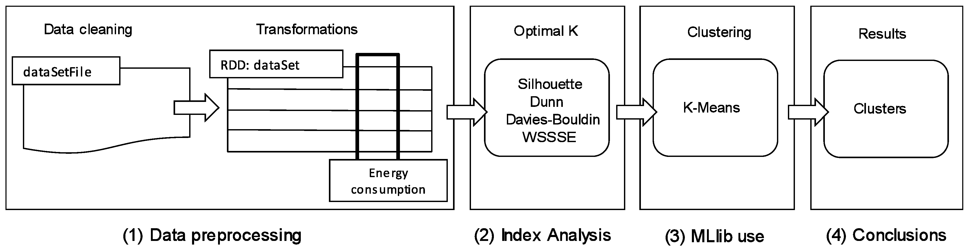
The key steps of the proposed methodology for obtaining consumption patterns are shown in Figure 1.
3.1. First Phase: Data Preprocessing
The first phase consists in data preprocessing. The objective of this phase is to clean and perform transformations in the original dataset to create a RDD variable, which can be distributed in a cluster and processed by Spark. The original dataset was obtained from the processing of several CSV files. These files contained records in the form of time series of power consumption data from six buildings of a public university. Data were extracted from the smart meters installed in the buildings. The smart meters collected electricity consumption records every 15 min from 2011 to 2016. Each row of the starting RDD variable is composed of five values: the name of the building, the date and time (separated into five values), and the energy consumption data at that time. In the data cleansing phase, our application pre-processed the rows containing missing records and accumulated consumption data so that correct learning models could be created in the next phases. This cleaning phase will be discussed extensively in the results section.
Before creating the model, it is necessary to perform a transformation in the original dataset by grouping the energy consumption series into rows of 96 records corresponding to a day. As each hour of the day contains four measurements, the original dataset has a total of 823,776 records, which are grouped per day generating a set with a total of 8581 instances.
In order to be able to identify which day a given result belongs to after applying clustering techniques, we will enter a unique identifier for each instance. This identifier is defined by combining the name of the building with the numerical date on which the measurements were taken.
Thus, each row of the RDD will finally contain a unique identifier and the 96 electric consumption records, in order to obtain conclusions associated with a particular day and building.
3.2. Second Phase: Obtaining the Optimal Number of Clusters
The second phase of the methodology consists in obtaining the optimal number of clusters for the dataset by analysing and interpreting various CVIs. However, some CVIs have limitations to be applied to large datasets due to the computational costs of quadratic complexity. This cost could take much longer to apply than the clustering algorithm used in this study. For this reason, we have applied big data clustering validity indices (BD-CVIs) [11].
In this paper we analyze the results of four BD-CVIs. Three of them are based on traditional CVIs—the BD-Silhouette, BD-Dunn and Davies-Bouldin indices—and the other is based on the Within Set Sum of Square Error (WSSSE) index offered by the MLlib. These BD-CVIs will be defined below. Let be the space of the objects with a given distance d. Let be a set of clusters so that and . Let be the centroid of and the centroid of .
BD-Silhouette: This index [11] is defined as the difference between inter-cluster and intra-cluster distances, divided by the maximum of them. The inter-cluster distance is the average of distances between each cluster centroid and global centroid . It is defined by:
The intra-cluster distance is defined as the average of the sum of the distances between each point and the centroid of the cluster to which it belongs. It is defined by the following equations:
Therefore, the BD-Silhouette index is defined as follows:
This value can range from −1 to 1 depending on the separation and consistency of the clusters. At the negative end, it will take the value −1 when there is only one cluster, and at the positive end, it will take the value 1 when there is a cluster for each of the dataset elements. In order to find an optimal value, it is necessary to look for the lowest possible K that maximizes the coherence and consistency of the cluster, being this the first maximum of the BD-Silhouette index.
BD-Dunn: This index [11] relates the maximum distance between all the points belonging to the same cluster and its corresponding centroid, and the minimum distance between these centroids and the global centroid.
This value is 0 if there is only one cluster and tends to zero when the number of clusters increases. Therefore, a maximum value in the BD-Dunn graph implies a higher quality of the clusters.
Davies-Bouldin: This index [31] assesses how distant clusters can be in order to make them of higher quality. Therefore, we will choose the first minimum of the Davies-Bouldin value chart to create a better model. The index is defined as follows:
where and are represented in Equation (2), and is the distance between the centroids and .
Within Set Sum of Square Errors (WSSSE): This index [32] is implemented in the MLlib. It is a measure of cluster cohesiveness and it calculates the sum of the distances from each point to the centroid of its cluster.
The optimal k is generally the one with a global minimum or the result after applying the “elbow method” to the WSSSE graph [33].
Majority Voting Methodology
The aim is to apply this group of indices to the complete set of data so that we can validate them and also obtain the optimal number of clusters K, which will be used as an input parameter of the parallelized k-means algorithm. In this sense, this work proposes a methodology of majority voting [34], which combines the results obtained of the application of the four indices above as a single result.
The voting strategy is now explained. The application of each of the indices separately to the complete dataset generates a graph that will show maxima or minima indicating the optimal number of clusters according to each case. Therefore, each of the graphs will have a first best value, a second best value, a third best value, and so on.
The voting system will evaluate the best results of all indices so that we extract as a result of the optimal k number of clusters to group our dataset.
There is a favourable and ideal situation: that all indices coincide with the best value or that most (i.e., at least three) coincide. In this case, we will take this value as the optimum k.
However, a second situation may arise: there are no coincidences or these are the minority (that is, fewer than three). When this case occurs, in addition to the first best values, the second best results of the four indices will be also considered. If a majority is not reached, we will study the third best results, and so on until we find a majority that matches. The selected k will then be the one that is repeated most times until the majority is found.
An example of the application of this system is shown in Table 1. In this case, the second situation occurs: only the BD-Dunn (six clusters) and Davies-Bouldin (six clusters) indices offer the same result (i.e., the minority of the first best results), resulting in the application of BD-Silhouette (four clusters) and WSSSE (seven clusters) indices in a manner different from the first two. At this point, we will have to look at the second best results to obtain the optimal number of clusters. If we look at the second best values, BD-Silhouette index coincides with BD-Dunn and Davies-Bouldin indices, since it offers six clusters as the second best result. Therefore, we will have found a majority (i.e., at least three matches), observing the first and second best results of the validity indices.
3.3. Third Fase: MLlib
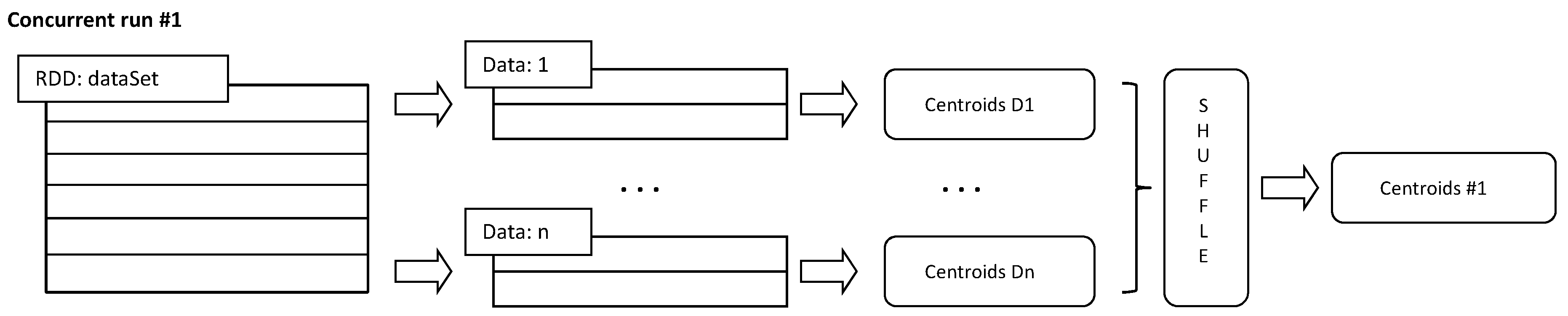
Once the optimal number of clusters k for the dataset has been obtained, the clustering algorithm can be applied. The algorithm used for discovering patterns from the dataset is the k-means [9]. This algorithm is a parallelized version of the k-means included in the MLlib of Apache Spark. This clustering algorithm is based on the classic k-means algorithm and has been developed to extract patterns in parallel and distributed systems.
Figure 2 shows how a run of the k-means works. First, the RDD object containing the complete dataset is distributed in several slave nodes for the execution of k-means, obtaining initial centroids n. Second, the Apache Spark engine shuffles the resulting n centroids for each run. Finally, the k-means algorithm computes the WSSSE index in each partition for each centroid, returning the one that minimizes the WSSSE as the best. It is worth remembering that there are as many centroids as there are concurrent executions. Figure 2 is representative of one execution.
3.4. Fourth Phase: Evaluation
The last phase corresponds to interpret and evaluate the results obtained after the application of k-means with the optimal number of clusters to the dataset.
We will obtain and analyze different types of results to obtain electric consumption patterns in big data time series. We will obtain the distribution of instances in each cluster and the centroids of the daily electricity consumption clusters.
Although clustering is considered an unsupervised learning technique, a clustering validity analysis has been carried out in this study, using features of the instances such as a type of day, season, or building as labels. Clustering results are merged with the features that each instance could have. Table 2 shows an example of the data that will be analysed Each row represents an instance of the dataset, i.e., the electricity consumption of a day, and the column cluster indicates the cluster assigned to that consumption. Also, each instance includes the features to be analysed as the building in which electricity was consumed, the season of the year, and the day of the week or non-working day.
With this information, we can see how the clusters are built regarding the features. Following our example, we can observe how the buildings are distributed by clusters, check out in which cluster there are more days off, or determine if the clusters are influenced by the season of the year. Based on this reasoning, we will draw the general conclusions using percentages of the distribution of buildings in the k clusters.
We will also conduct a study of several synthetic big datasets. Starting from the base of the original set, we will multiply its original size with the objective of checking the efficiency in computing time of the proposed methodology.
All the experiments were executed in Amazon Web Services (AWS) Elastic Map Reduce using two different hardware scenarios:
- Five instances of with Intel Xeon E5-2670 v2 (Ivy Bridge) processors with 8 CPUs, 15 GB RAM, and 2 SSDs of 40 GB each.
- Five instances of with Intel Xeon E5-2670 v2 (Ivy Bridge) processors with 16 CPUs, 30 GB RAM, and 2 SSDs of 80 GB each.
4. Results
This section is organized as follows. Section 4.1 describes the dataset and the preprocessing carried to be out. Section 4.2 shows the results obtained when applying the four clustering validity indices. Finally, Section 4.3 presents the results of the clustering analysis obtained by the k-means.
4.1. Description of the Dataset
As described in the previous section, the first phase is a previous treatment of the raw data. The initial dataset is made up of measurements of electricity consumption with a 15-min frequency taken over six consecutive years. However, these measurements present missing values, which were treated as follows.
Being a time series of 96 elements corresponding to one-day measurements, we find certain empty measurements with zero value. These empty measurements occurred due to point-based errors in the smart meters. In these cases, these zero values precede a very high measurement, well above the average of measurements in that daily interval, corresponding to the accumulation of missing measurements in the previous intervals.
For this reason, these empty values were modified with the mean corresponding to the division of this high value by the number of empty values.
As a result of this cleaning, a RDD variable composed of 8581 rows and 97 columns (the first one with the unique identifier and the remaining ones with electrical consumption measurements) will be analyzed in this work.
The RDD object contains electricity consumption measurements of sensors from the following buildings of Pablo de Olavide University of Sevilla in Spain:
- Building 1—Backup data processing centre (DPC).
- Building 11—Office for professors and classrooms on the ground floor.
- Building 12—Administration services.
- Building 20—Research centre of developmental biology.
- Building 21—Experimental research services.
- Building 42—Old kindergarten (closed since 2010).
- Building 44—Administration services.
- Cafeteria—Cafeteria.
4.2. Cluster Validity Indices Analysis
In this section, the BD-CVIs have been applied to determine the optimal number of clusters to discover useful patterns of electricity consumption in the different buildings of the university.
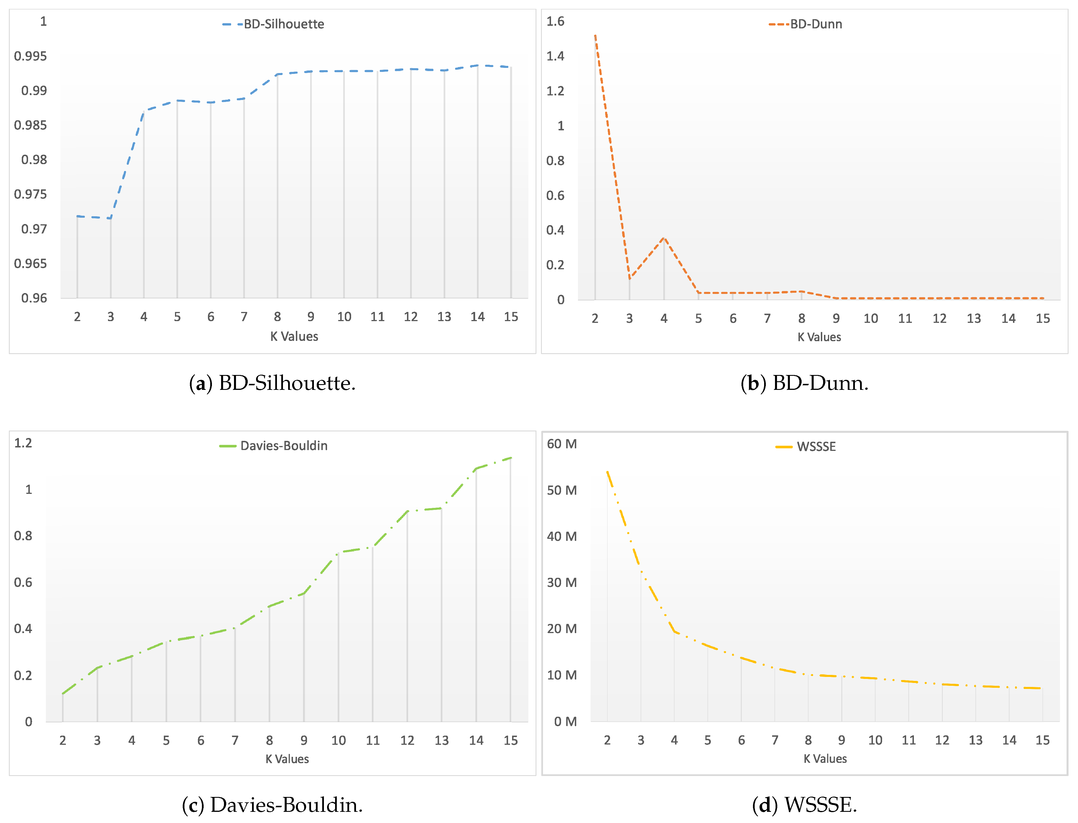
Figure 3 shows the results of the clustering validity indices described in Section 3.2. The results for the BD-Silhouette index are shown in Figure 3a. It can be observed that its curve reaches two local maxima at four and eight. Figure 3b is the BD-Dunn graph and shows local maximum values at four and eight also. The Davies-Bouldin index (Figure 3c) does not show any clear results. However, the curve draws some changes of tendency at 10, 12, and 14, which could be valid results. Figure 3d corresponds to the WSSSE index and draws a stabilization of its values at four and eight. Note that M means millions.
Table 3 shows the results of the BD-CVIs. According to the majority voting method, BD-CVIs suggest that four and eight could be optimal numbers of clusters for the dataset.
4.3. Clustering Results
Clustering results are presented in this Section. As two possible values for the number of clusters have been obtained, this section is divided into two subsections. Section 4.3.1 and Section 4.3.2 describe the results when considering four and eight clusters as the optimal number of clusters, respectively.
4.3.1. Analysis of Results: Four Clusters
Table 4 shows the percentage of instances belonging to each cluster. It shows that cluster 1 is the densest, containing 72% of the instances. On the other hand, the consumption centroids for each cluster are displayed in Figure 4. It can be concluded that there are two groups of clusters depending on the consumption level:
- Clusters 2 and 3 with the highest consumptions but with few instances (7% and 4%, respectively).
- Clusters 1 and 4 with the lowest consumptions and the largest percentage of instances (72% and 18%, respectively).
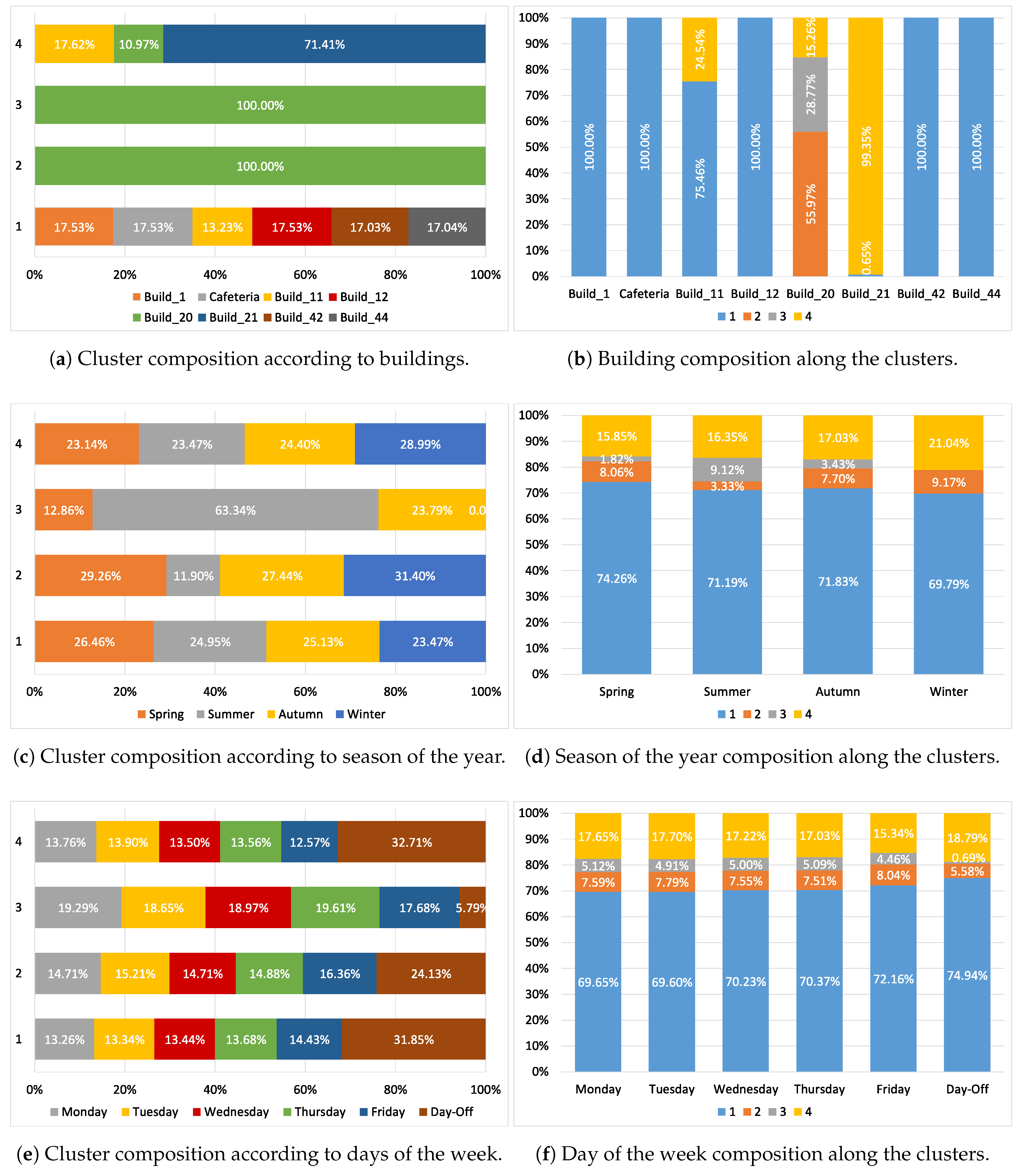
Figure 5 shows an analysis of the clusters according to the features buildings, seasons of the year and days of the week. There are two kinds of graphs: Figure 5a,c and e (left side) represent how the clusters are composed of the features, where the bars symbolize the clusters and the colours are the different features. Figure 5b,d and f (right side) represent the presence of the different features in the clusters, where the different features are the columns and the clusters are represented by colours.
Figure 5a,b presents the composition of the clusters according to the buildings. Figure 5a shows how the clusters are composed of the different buildings. It can be noticed that clusters 2 and 3 consist of the building 20. Cluster 4 is mainly formed by building 21 -71.41%- and the cluster 1 is equally distributed among all the buildings except buildings 20 and 21. Figure 5b shows the composition of the buildings depending on the clusters. It should be noted that all the buildings, except buildings 20 and 21, have instances in cluster 1, and buildings 1, 12, 42, 44 and cafeteria are just in it.
Figure 5c,d depict a characterization of the clusters according to the feature of the seasons of the year. It is worth noting that cluster 3 is a mainly summer cluster with no instances from winter, and cluster 2 is be the opposite, with few instances of summer and a 31.40% of winter.
Figure 5e,f present the patterns related to the days of the week. It should be highlighted that the percentage of instances is similar during the weekdays. Mainly, the differences exist between the working days and non-working days. Cluster 3 may be considered a working day cluster because the non-working days’ instances are just 5.79%. Besides, clusters 1 and 4 have a high rate of instances of non-working days (31.85% and 32.7%, respectively). This fact is consistent with the fact that clusters 1 and 4 were characterized as low-consumption clusters.
Table 5 present the patterns discovered when using four clusters. The characterization of the clusters related to the selected features is summarized as follows:
- Clusters 1 has low consumption and a significant number of instances corresponding to non-working days.
- Cluster 4 has low consumption, and consists of buildings 11 (offices), 20, and 21 (research centres) and instances with a greater presence in non-working days.
- Cluster 2 and 3 have high consumption and both contain building 20, but they are opposites in terms of seasons and days of the week. On the one hand, cluster 2 may be considered a non-summer cluster with a larger number of instances corresponding to non-working days. Although the cluster 2 has a large number of non-working days, the electricity consumption is high because building 20 is dedicated to experimental research. On the other hand, cluster 3 is considered a non-winter cluster, defined by weekdays mainly.
4.3.2. Analysis of Results: Eight Clusters
Table 6 shows the number of instances belonging to each cluster after applying k-means with eight clusters. The results show that there are two major clusters, as 39% of the instances belong to clusters 1, 32% to cluster 7 and the rest of the clusters do not reach percentages of 10% each.
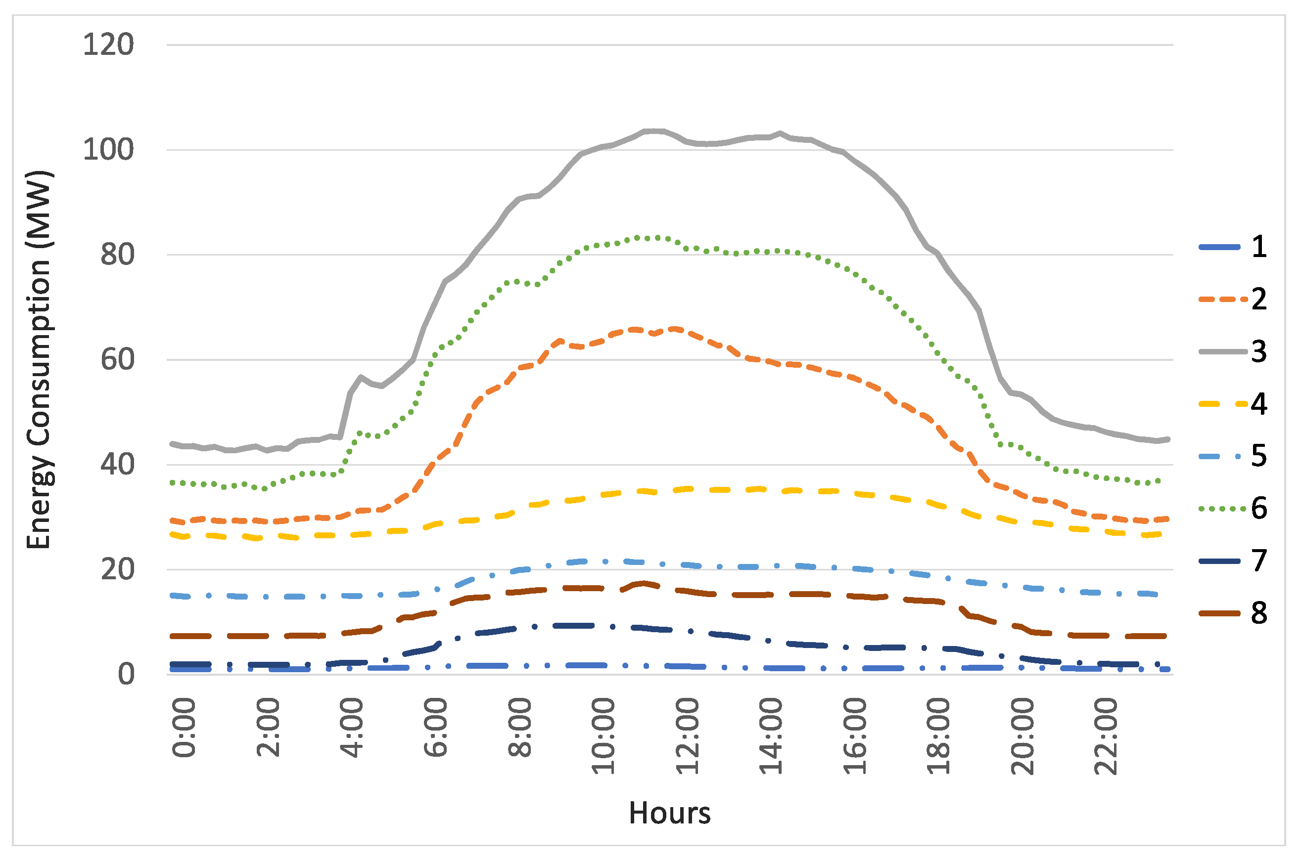
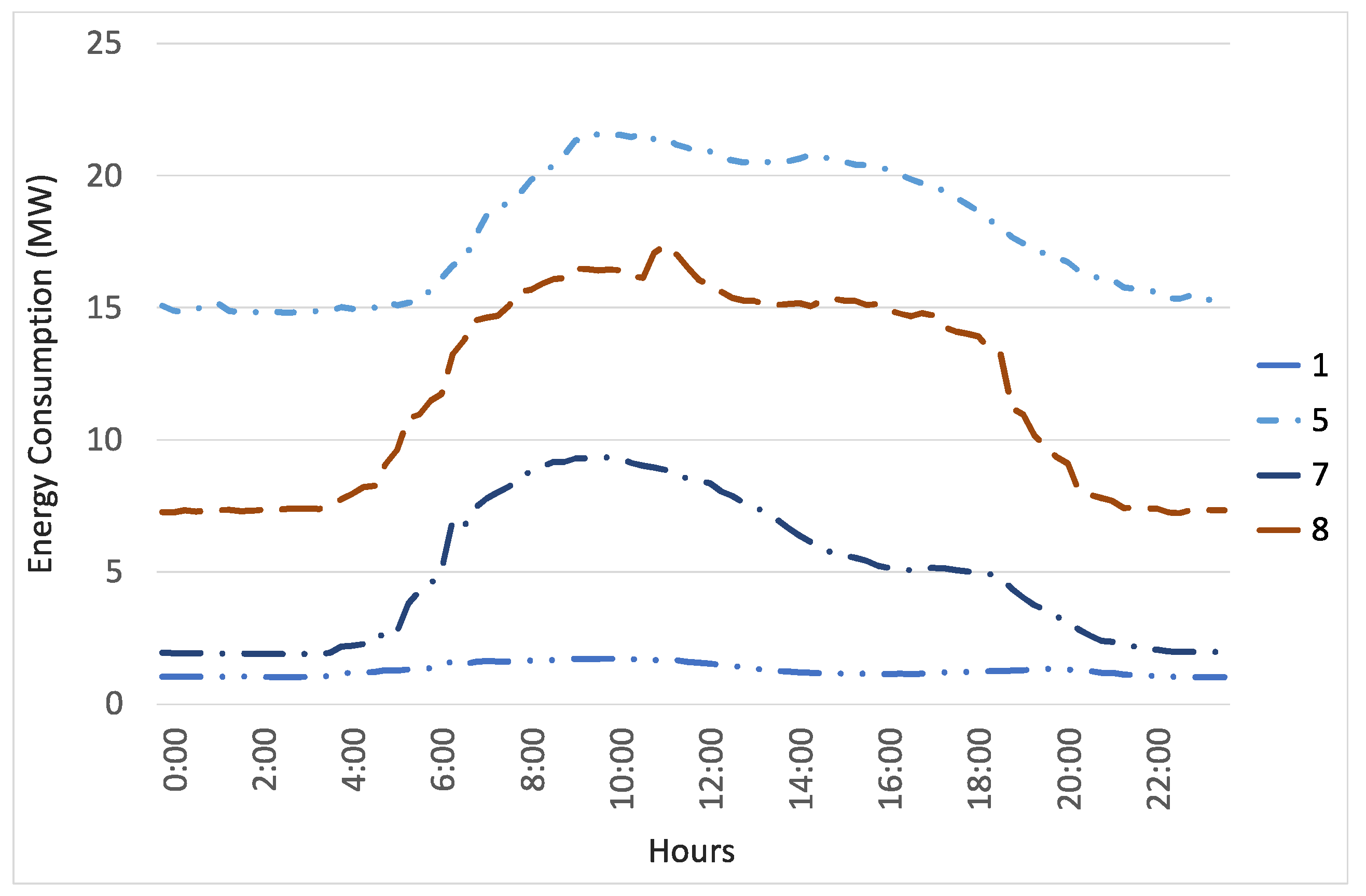
Figure 6 and Figure 7 display the centroids of the clusters representing the average consumptions (in MW), which belong to each cluster within a full day. Figure 6 shows the centroids of all the clusters while Figure 7 shows the centroids with lower consumptions in more detail. Figure 6 reveals that clusters 2, 3, and 6 have a very high consumption compared to the rest of the clusters. These three clusters have higher consumptions during daylight hours, although the night hours still have a high consumption. Cluster 4 also has a very high consumption, and it remains constant during the day. Clusters 5, 7, and 8 have lower consumptions, which are higher during the daylight hours and much lower during the night. Cluster 1, that contains the largest number of instances, has a consumption close to zero during the entire day.
Figure 8 shows an analysis of the clusters obtained when using eight clusters depending on features such as buildings, seasons of the year, and days of the week.
Figure 8a illustrates how the clusters are composed of the buildings in percent. Clusters 2, 3, 4 and 6 are mainly composed of building 20. Besides, cluster 1 is made up of all the buildings except buildings 20 and 21. Cluster 5 consists of the building 21 mainly. The building 21 is also present in cluster 8, that shares half of the instances with building 11. Cluster 7 is formed by instances from all the buildings except buildings 20, 21, and 42. Figure 8b presents the composition of the buildings according to the clusters. It may be highlighted that buildings 1, 11, 12, 44 and the cafeteria belong to clusters 1 and 7. Moreover, the buildings 20 and 21 are just the opposite because they belong to different clusters. It is also worth mentioning that the building 42 has all the instances in cluster 1. This is due to building 42 being the old kindergarten closed since 2010, and therefore, this building has no electricity consumption.
Figure 8c presents how the clusters are composed of seasons of the year. It can be appreciated that clusters generally have instances equally distributed over the seasons with some exceptions. For instance, cluster 2 has instances during all the seasons but summer, and the opposite situation is found in cluster 3, which has more instances corresponding to summer days. Furthermore, clusters 2, 4, and 5 have a percentage of instances slightly higher in winter: 36.02%, 34.31%, and 32.46%, respectively. It worth mentioning that cluster 6 is composed of non-winter instances as just a 0.51% of instances correspond to winter and 41.92% to summer.
Figure 8e shows the distribution of the days of the week depending on the clusters. It is worth noting that clusters 1 and 4 are mainly composed of non-working days, just the opposite to clusters 3 and 7 that only have 3.51% and 5.82% of day-off instances, respectively. Figure 8f presents the percentage of instances of each cluster composing each type of day. It can be emphasized that days off are mainly composed of cluster 1 instances, while the rest of days are mostly formed by cluster 7.
Table 7 provides a characterization of the clusters obtained when using 8 clusters by means of the features analysed A summary is described below:
- Cluster 1 contains the instances with the lowest consumption and that are constant throughout the day. It is composed of all the buildings except buildings 20 and 21 (research centres). The instances are mostly non-working days and they are distributed uniformly over all seasons of the year.
- Clusters 2, 3, 4, and 6 are composed of building 20. These clusters contain the highest consumption during daylight hours. Clusters 2 and 6 include instances from all the days of the week, while clusters 3 and 4 just have instances from working days and non-working days, respectively. Most of the instances of the cluster 2 are non-summer instances, and cluster 3 is just the opposite because it includes summer instances mainly.
- Cluster 5 is composed of building 21. It is characterized by a low consumption which is higher during daylight hours. In addition, it contains instances of all the days of the week but slightly more for non-working days.
- Cluster 7 consists of all the buildings, except 20, 21, and 42. It represents a low consumption higher during daylight hours and working days.
- Cluster 8 is formed by the buildings 11 (offices) and 21. It represents low consumption but higher during daylight hours and non-working days.
5. Execution Times
This section provides the computing times using different synthetic big data to evaluate the scalability of the proposed methodology. To this end, the set of the electricity consumptions from the eight buildings located on the university campus has been exponentially increased, with the aim of simulating a neighbourhood, a town, a city or a metropolis.
Let us remember that the data comes from smart meters every 15 min for six years for eight buildings. Mathematical operations defined in set theory such as union, distinct, or join, which are supported by Spark technology, were used in order to transform datasets into exponentially bigger ones. In particular, the input datasets were generated by means of union operations from the original ones.
Table 8 shows computing times obtained by the proposed methodology using synthetic datasets for two different hardware configurations. Each row describes information about each of the generated datasets such as the number of buildings, total number of instances, size of the file and runtimes measured in hours. shows runtimes using a five-node cluster with 8 CPUs and 15 GB RAM, and the column is the second hardware scenario where there is a five-node cluster composed of 16 CPUs and 30 GB RAM.
On the one hand, in the first hardware scenario, execution times are negligible up until the dataset of 11.63 GB composed of 16,384 buildings. The largest dataset with 131,072 buildings, big data that could represent a big metropolis, had a time of 5.2325 h. On the other hand, the second hardware configuration keeps slight runtimes, at 0.0995 h, up until the dataset with 65,536 buildings, with 1.1985 h for the largest dataset. It should be highlighted that the first configuration obtained reasonable times, but using a more powerful hardware configuration, times are reduced considerably. For the largest dataset, execution time has been reduced up to 5 times and about 40 times for the dataset with 65,536 buildings.
Computational times of the different processes in the methodology are proportional in the two hardware configurations. Taking into account all the phases of the methodology, obtaining the optimum number of clusters is the process that takes the longest, occupying 72% of the total time. This is because it is an iterative process in which k-means is launched along the indices n times, where n is the maximum number of clusters we could assume. Within this process, k-means takes 85%, and the rest of the time is used to calculate the values of the clustering validity indices. The next phases that take longer are clustering and preprocessing analysis, lasting 13% and 11%, respectively. Finally, the calculation of the k-means takes the shortest time, since it simply launches the algorithm with already preprocessed data and an optimal number of clusters.
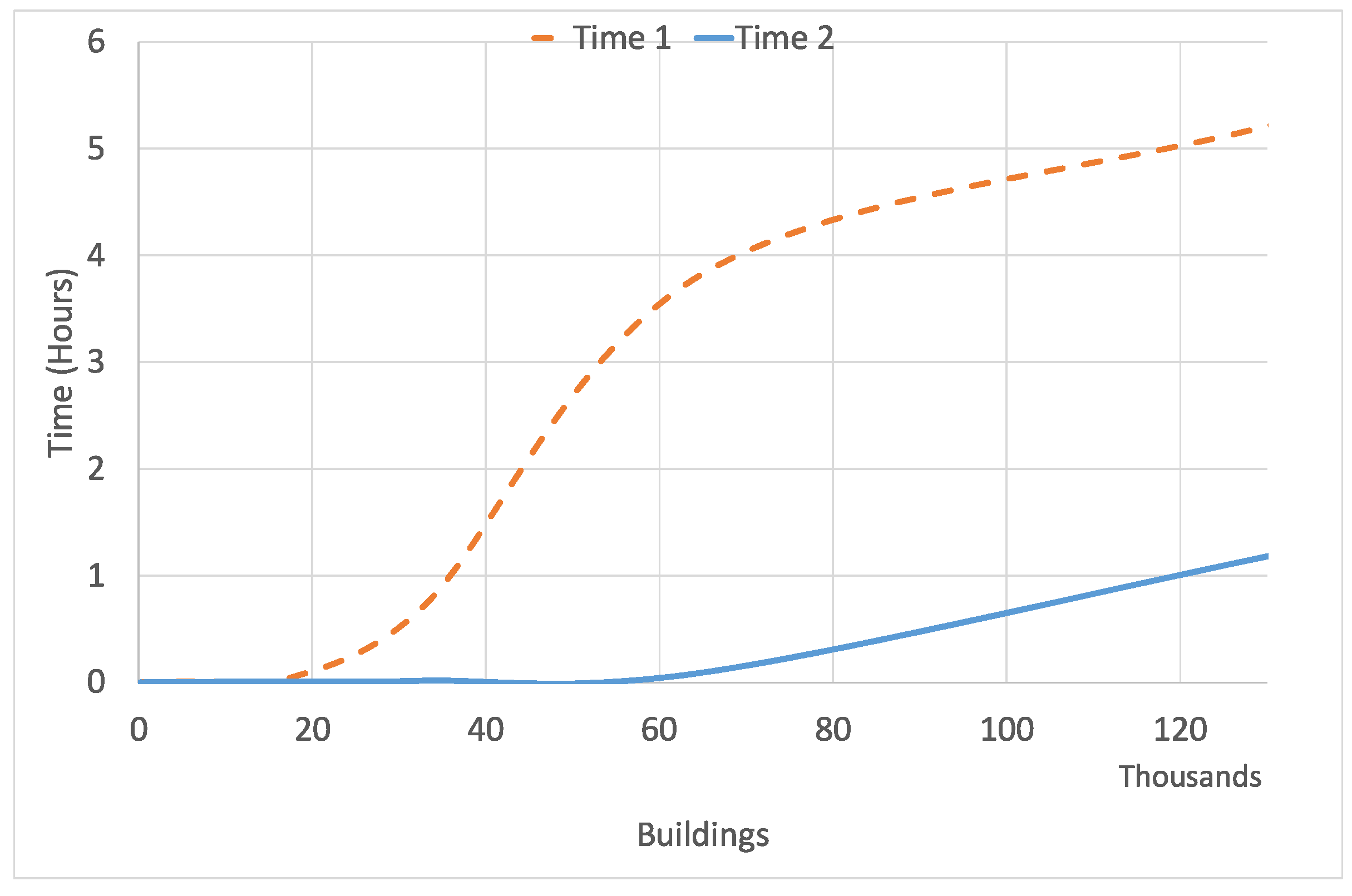
Figure 9 graphically shows runtimes in hours when increasing the number of buildings for the two different hardware configurations. As it can be noticed, both runtimes are similar using datasets with less than 20,000 buildings, but the difference between both configurations is quite remarkable for 60,000 buildings. In particular, was 40 times larger than . As it can be seen, results show that techniques described in this paper can be applied to optimize the electricity consumption of a smart city within a reasonable time.
6. Conclusions
A detailed understanding of energy consumption patterns of buildings is essential for smart cities. On the one hand, electricity companies can improve the pricing policies and offer customized packages for certain types of communities. On the other hand, public administrations can optimize resources by contracting certain hourly rates of discrimination offered by the main electricity companies in the countries. A joint application of the methodology proposed in this work by energy companies and public administrations can bring benefits to the community as a whole since energy saving is essential to reduce the impact on climate change and promote sustainable development. In this context, we propose a work methodology to detect patterns from big data time series, as this type of data is generated by modern smart cities through the increasingly common smart meters.
In this paper, a model based on the k-means algorithm was designed for this purpose using the distributed computing advantages of Apache Spark. Firstly, a study of four CVIs optimized for parallelization—the DB-Dunn, DB-Silhouette, Davies-Bouldin and WSSSE indices—was carried out. From these indices, a majority voting strategy was applied in order to choose the optimal number of clusters. This study returned two possible values for the number of clusters and an in-depth analysis of the patterns for both cases was performed.
Next, patterns were characterized according to the building, type of consumption (high, low, daytime or constant), the season of the year, and day of the week (including days off). A valuable interpretation of the patterns obtained has been provided. Namely, the consumption behaviour of buildings depends mainly on their characteristics (administration buildings, research centres, classrooms or leisure facilities) and the hours during the day which they are used. In addition, it has been shown that there is a strong relationship between temperature and consumption, and a high impact of holiday periods in the academic calendar.
Finally, several synthetic datasets were generated from the original dataset. These datasets were used to measure computing times required to discover patterns using the proposed methodology. Results showed a linear relationship between runtimes and size of datasets. In fact, the execution time for the largest dataset considering big data is less than 4 h. Thus, in the hypothetical case of obtaining a dataset with six-year measurements for 65,536 buildings, the runtime is computationally suitable.
Future work will focus on two aspects: firstly, to discover consumption patterns in big data using other additional variables (such as price or type of consumer), and secondly, the prediction of electricity consumption from big data using distributed technology such as Apache Spark. The complete methodology proposed in this paper allows us to lay the foundations for the use of different prediction algorithms, once the original data set has been clustered. In this sense, algorithms in distributed technology are being developed to obtain predictions with high accuracy.
These two approaches will support the economic and political decision making of different public administrations, as well as the personalization of products by private organizations (energy companies, for example), increasingly involved in tracking their resources to obtain valuable information in the context of smart cities.
Acknowledgments
This work has been supported by the Spanish Ministry of Economy and Competitiveness and Junta de Andalucía under projects TIN2014-55894-C2-R, TIN2017-88209-C2-R and P12-TIC-1728. J.M.L.-R. holds a FPI scholarship from the Spanish Ministry of Economy and Competitiveness.
Author Contributions
R.P.-C. and J.M.L.-R. implemented the methodology and drafted the manuscript; J.C.R. conceived and designed the experiments; A.T. and F.M.-Á. participated in the elaboration of the manuscript; all authors read, edited and approved the manuscript.
Conflicts of Interest
The authors declare no conflict of interest.
Abbreviations
The following abbreviations are used in this manuscript:
| MLlib | Machine Learning Library |
| CVI | Cluster Validity Index |
| BD-CVI | Big Data Cluster Validity Index |
| RDD | Resilient Distributed Dataset |
| DPC | Data Processing Centre |
| AWS | Amazon Web Services |
References
- Nuaimi, E.A.; Neyadi, H.A.; Mohamed, N.; Al-Jaroodi, J. Applications of big data to smart cities. J. Internet Ser. Appl. 2015, 6, 1–15. [Google Scholar] [CrossRef]
- Gungor, V.C.; Sahin, D.; Kocak, T.; Ergut, S.; Buccella, C.; Cecati, C.; Hancke, G.P. Smart Grid Technologies: Communication Technologies and Standards. IEEE Trans. Ind. Inf. 2011, 7, 529–539. [Google Scholar] [CrossRef]
- Fernández, A.; del Río, S.; López, V.; Bawakid, A.; del Jesús, M.J.; Benítez, J.M.; Herrera, F. Big Data with Cloud Computing: An insight on the computing environment, MapReduce, and programming frameworks. Wiley Interdiscip. Rew. Data Min. Knowl. Discov. 2014, 4, 380–409. [Google Scholar] [CrossRef]
- Orgaz, G.B.; Jung, J.J.; Camacho, D. Social big data: Recent achievements and new challenges. Inf. Fusion 2016, 28, 45–59. [Google Scholar] [CrossRef]
- Dean, J.; Ghemawat, S. MapReduce: Simplified Data Processing on Large Clusters. Commun. ACM 2008, 51, 107–113. [Google Scholar] [CrossRef]
- Zaharia, M.; Chowdhury, M.; Franklin, M.J.; Shenker, S.; Stoica, I. Spark: Cluster Computing with Working Sets. In Proceedings of the 2Nd USENIX Conference on Hot Topics in Cloud Computing; HotCloud’10; USENIX Association: Berkeley, CA, USA, 2010; p. 10. [Google Scholar]
- Zaharia, M.; Chowdhury, M.; Das, T.; Dave, A.; Ma, J.; McCauley, M.; Franklin, M.J.; Shenker, S.; Stoica, I. Resilient Distributed Datasets: A Fault-tolerant Abstraction for In-memory Cluster Computing. In Proceedings of the 9th USENIX Conference on Networked Systems Design and Implementation; NSDI’12; USENIX Association: Berkeley, CA, USA, 2012; p. 2. [Google Scholar]
- Meng, X.; Bradley, J.; Yavuz, B.; Sparks, E.; Venkataraman, S.; Liu, D.; Freeman, J.; Tsai, D.; Amde, M.; Owen, S.; et al. MLlib: Machine Learning in Apache Spark. J. Mach. Learn. Res. 2016, 17, 1–7. [Google Scholar]
- Bahmani, B.; Moseley, B.; Vattani, A.; Kumar, R.; Vassilvitskii, S. Scalable K-means++. Proc. VLDB Endow. 2012, 5, 622–633. [Google Scholar] [CrossRef]
- Arbelaitz, O.; Gurrutxaga, I.; Muguerza, J.; PéRez, J.M.; Perona, I.N. An Extensive Comparative Study of Cluster Validity Indices. Pattern Recogn. 2013, 46, 243–256. [Google Scholar] [CrossRef]
- Luna-Romera, J.M.; García-Gutiérrez, J.; Martínez-Ballesteros, M.; Santos, J.C.R. An approach to validity indices for clustering techniques in Big Data. Prog. Artif. Intell. 2017, 7, 1–14. [Google Scholar] [CrossRef]
- Martínez-Álvarez, F.; Troncoso, A.; Riquelme, J.C.; Ruiz, J.S.A. Energy Time Series Forecasting Based on Pattern Sequence Similarity. IEEE Trans. Knowl. Data Eng. 2011, 23, 1230–1243. [Google Scholar] [CrossRef]
- Tuballa, M.L.; Abundo, M.L. A review of the development of Smart Grid technologies. Renew. Sustain. Energy Rev. 2016, 59, 710–725. [Google Scholar] [CrossRef]
- Calvillo, C.; Sánchez-Miralles, A.; Villar, J. Energy management and planning in smart cities. Renew. Sustain. Energy Rev. 2016, 55, 273–287. [Google Scholar] [CrossRef]
- Sun, Y.; Song, H.; Jara, A.J.; Bie, R. Internet of Things and Big Data Analytics for Smart and Connected Communities. IEEE Access 2016, 4, 766–773. [Google Scholar] [CrossRef]
- Xu, J.; Zhang, R. CoMP Meets Smart Grid: A New Communication and Energy Cooperation Paradigm. IEEE Trans. Vehicular Technol. 2015, 64, 2476–2488. [Google Scholar] [CrossRef]
- Wijk, J.J.V.; Selow, E.R.V. Cluster and calendar based visualization of time series data. In Proceedings of the IEEE Symposium on Information Visualization, San Francisco, CA, USA, 24–29 October 1999; pp. 4–9. [Google Scholar]
- Martínez-Álvarez, F.; Troncoso, A.; Riquelme, J.C.; Riquelme, J.M. Partitioning-Clustering Techniques Applied to the Electricity Price Time Series. In Proceedings of the Intelligent Data Engineering and Automated Learning, Birmingham, UK, 16–19 December 2007; pp. 990–999. [Google Scholar]
- Martínez-Álvarez, F.; Troncoso, A.; Riquelme, J.C.; Riquelme, J.M. Discovering patterns in electricity price using clustering techniques. In Proceedings of the International Conference on Renewable Energy and Power Quality, Sevilla, Spain, 28–30 march 2007; pp. 245–252. [Google Scholar]
- Keyno, H.S.; Ghaderi, F.; Azade, A.; Razmi, J. Forecasting electricity consumption by clustering data in order to decline the periodic variable’s affects and simplification the pattern. Energy Convers. Manag. 2009, 50, 829–836. [Google Scholar] [CrossRef]
- Hernández, L.; Baladrón, C.; Aguiar, J.M.; Carro, B.; Sánchez-Esguevillas, A. Classification and Clustering of Electricity Demand Patterns in Industrial Parks. Energies 2012, 5, 5215–5228. [Google Scholar] [CrossRef]
- Fahad, A.; Alshatri, N.; Tari, Z.; Alamri, A.; Khalil, I.; Zomaya, A.Y.; Foufou, S.; Bouras, A. A Survey of Clustering Algorithms for Big Data: Taxonomy and Empirical Analysis. IEEE Trans. Emerg. Top. Comput. 2014, 2, 267–279. [Google Scholar] [CrossRef]
- Ding, R.; Wang, Q.; Wang, Q.; Dang, Y.; Fu, Q.; Zhang, H.; Zhang, D.; Ding, J. YADING: Fast Clustering of Large-Scale Time Series Data. Proc. Very Large Data Bases 2015, 8, 473–484. [Google Scholar] [CrossRef]
- Rakthanmanon, T.; Campana, B.; Mueen, A.; Batista, G.; Westover, B.; Zhu, Q.; Zakaria, J.; Keogh, E. Addressing Big Data Time Series: Mining Trillions of Time Series Subsequences Under Dynamic Time Warping. ACM Trans. Knowl. Discov. Data 2013, 7, 1–31. [Google Scholar] [CrossRef]
- Zhao, W.; Ma, H.; He, Q. Parallel K-Means Clustering Based on MapReduce. In Cloud Computing; Jaatun, M.G., Zhao, G., Rong, C., Eds.; Springer: Berlin/Heidelberg, Germany, 2009; pp. 674–679. [Google Scholar]
- Capó, M.; Pérez, A.; Lozano, J.A. An Efficient Approximation to the K-means Clustering for Massive Data. Know.-Based Syst. 2017, 117, 56–69. [Google Scholar] [CrossRef]
- Melzi, F.N.; Same, A.; Zayani, M.H.; Oukhellou, L. A Dedicated Mixture Model for Clustering Smart Meter Data: Identification and Analysis of Electricity Consumption Behaviors. Energies 2017, 10, 1–21. [Google Scholar] [CrossRef]
- Deb, C.; Zhang, F.; Yang, J.; Lee, S.E.; Shah, K.W. A review on time series forecasting techniques for building energy consumption. Renew. Sustain. Energy Rev. 2017, 74, 902–924. [Google Scholar] [CrossRef]
- Singh, S.; Yassine, A. Big Data Mining of Energy Time Series for Behavioral Analytics and Energy Consumption Forecasting. Energies 2018, 11, 452. [Google Scholar] [CrossRef]
- Li, C.; Ding, Z.; Zhao, D.; Yi, J.; Zhang, G. Building Energy Consumption Prediction: An Extreme Deep Learning Approach. Energies 2017, 10, 1525. [Google Scholar] [CrossRef]
- Davies, D.L.; Bouldin, D.W. A Cluster Separation Measure. IEEE Trans. Pattern Anal. Mach. Intell. 1979, 1, 224–227. [Google Scholar] [CrossRef] [PubMed]
- Spark, A. Clustering—RDD-Based API—Spark 2.2.0 Documentation. 2017. Available online: https://spark.apache.org/docs/2.2.0/mllib-clustering.html#k-means (accessed on 20 December 2017).
- Ketchen, D.J.; Shook, C.L. The Application Of Cluster Analysis In Strategic Management Research: An Analysis And Critique. Strateg. Manag. J. 1996, 17, 441–458. [Google Scholar] [CrossRef]
- Koprinska, I.; Rana, M.; Troncoso, A.; Martínez-Álvarez, F. Combining pattern sequence similarity with neural networks for forecasting electricity demand time series. In Proceedings of the 2013 International Joint Conference on Neural Networks (IJCNN), Dallas, TX, USA, 4–9 August 2013; pp. 1–8. [Google Scholar]
Figure 1.
Proposed methodology. RDD: Resilient Distributed Dataset; MLlib: Machine Learning Library; WSSSE: Within Set Sum of Square Errors.
Figure 1.
Proposed methodology. RDD: Resilient Distributed Dataset; MLlib: Machine Learning Library; WSSSE: Within Set Sum of Square Errors.

Figure 2.
One concurrent execution of the k-means algorithm.

Figure 3.
BD-Silhouette, BD-Dunn, Davies-Bouldin, and WSSSE clustering validity indices for k values from 2 to 15.
Figure 3.
BD-Silhouette, BD-Dunn, Davies-Bouldin, and WSSSE clustering validity indices for k values from 2 to 15.

Figure 4.
Centroids of the electricity consumption clusters.

Figure 5.
Cluster analysis depending on buildings, seasons of the year and days of the week.

Figure 6.
Centroids of the electricity consumption clusters.

Figure 7.
Centroids of the clusters with lower consumptions.

Figure 8.
Cluster analysis depending on buildings, seasons of the year, and days of the week.

Figure 9.
A runtime comparison between the two different hardware configurations.


Table 1.
Majority voting methodology.
| Values | BD-Silhouette | BD-Dunn | Davies-Bouldin | WSSSE |
|---|---|---|---|---|
| First | 4 | 6 | 6 | 7 |
| Second | 6 | 8 | 9 | 15 |
| Third | 9 | 13 | 15 | 21 |
Table 2.
Example of a dataset along with assigned cluster and features.
| ID | Cluster | Building | Season | Day |
|---|---|---|---|---|
| 1 | 1 | Build_1 | Summer | Day off |
| 2 | 1 | Build_1 | Winter | Day off |
| 3 | 2 | Build_20 | Summer | Thursday |
| 4 | 1 | Build_42 | Summer | Friday |
| 5 | 3 | Build_1 | Autumn | Monday |
Table 3.
Majority voting from cluster validation indices (CVIs).
| Values | BD-Silhouette | BD-Dunn | Davies-Bouldin | WSSSE |
|---|---|---|---|---|
| First | 4 | 4 | 10 | 4 |
| Second | 8 | 8 | 12 | 8 |
| Third | - | - | 14 | - |
Table 4.
Instances along the clusters.
| Cluster | Total | Rate |
|---|---|---|
| 1 | 6161 | 72% |
| 2 | 605 | 7% |
| 3 | 311 | 4% |
| 4 | 1504 | 18% |
Table 5.
Cluster analysis for four clusters.
| Consumption | Buildings | Days | Seasons | |||||
|---|---|---|---|---|---|---|---|---|
| Cluster | High | Low | 11 | 20 | 21 | Non-Working Days | Non-Summer | Non-Winter |
| 1 | ✓ | ✓ | ||||||
| 2 | ✓ | ✓ | ✓ | ✓ | ||||
| 3 | ✓ | ✓ | ✓ | |||||
| 4 | ✓ | ✓ | ✓ | ✓ | ✓ | |||
Table 6.
Instances along the clusters.
| Cluster | Total | Rate |
|---|---|---|
| 1 | 3333 | 39% |
| 2 | 472 | 6% |
| 3 | 171 | 2% |
| 4 | 274 | 3% |
| 5 | 684 | 8% |
| 6 | 198 | 2% |
| 7 | 2715 | 32% |
| 8 | 734 | 9% |
Table 7.
Cluster analysis for eight clusters.
| Consumption | Days | Seasons | Buildings | ||||||||
|---|---|---|---|---|---|---|---|---|---|---|---|
| Cluster | High | Low | Diurnal | Working Days | Non-Working Days | Non-Summer | Summer | Non-Winter | 11 | 20 | 21 |
| 1 | ✓ | ✓ | ✓ | ||||||||
| 2 | ✓ | ✓ | ✓ | ✓ | |||||||
| 3 | ✓ | ✓ | ✓ | ✓ | ✓ | ||||||
| 4 | ✓ | ✓ | ✓ | ||||||||
| 5 | ✓ | ✓ | ✓ | ||||||||
| 6 | ✓ | ✓ | ✓ | ✓ | |||||||
| 7 | ✓ | ✓ | ✓ | ✓ | |||||||
| 8 | ✓ | ✓ | ✓ | ✓ | ✓ | ||||||
Table 8.
Computing times (in hours) using synthetic big data for two different hardware configurations.
Table 8.
Computing times (in hours) using synthetic big data for two different hardware configurations.
| Buildings | Instances | File Size | ||
|---|---|---|---|---|
| 16 | 17,162 | 10.3 MB | 0.0015 | 0.0015 |
| 32 | 34,324 | 20.5 MB | 0.0015 | 0.0016 |
| 64 | 68,648 | 41.2 MB | 0.0015 | 0.0014 |
| 128 | 137,296 | 82.4 MB | 0.0014 | 0.0015 |
| 256 | 274,592 | 190.1 MB | 0.0018 | 0.0017 |
| 512 | 549,184 | 380.9 MB | 0.0021 | 0.0015 |
| 1024 | 1,098,368 | 744.1 MB | 0.0023 | 0.0022 |
| 2048 | 2,196,736 | 1.45 GB | 0.0037 | 0.0020 |
| 4096 | 4,393,472 | 2.91 GB | 0.0067 | 0.0023 |
| 8192 | 8,786,944 | 5.81 GB | 0.0094 | 0.0054 |
| 16,384 | 17,573,888 | 11.63 GB | 0.0156 | 0.0091 |
| 32,768 | 35,147,776 | 23.26 GB | 0.7078 | 0.0162 |
| 65,536 | 70,295,552 | 46.52 GB | 3.8555 | 0.0995 |
| 131,072 | 140,591,104 | 93.03 GB | 5.2325 | 1.1985 |
© 2018 by the authors. Licensee MDPI, Basel, Switzerland. This article is an open access article distributed under the terms and conditions of the Creative Commons Attribution (CC BY) license (http://creativecommons.org/licenses/by/4.0/).
Share and Cite
MDPI and ACS Style
Pérez-Chacón, R.; Luna-Romera, J.M.; Troncoso, A.; Martínez-Álvarez, F.; Riquelme, J.C. Big Data Analytics for Discovering Electricity Consumption Patterns in Smart Cities. Energies 2018, 11, 683. https://doi.org/10.3390/en11030683
AMA Style
Pérez-Chacón R, Luna-Romera JM, Troncoso A, Martínez-Álvarez F, Riquelme JC. Big Data Analytics for Discovering Electricity Consumption Patterns in Smart Cities. Energies. 2018; 11(3):683. https://doi.org/10.3390/en11030683
Chicago/Turabian StylePérez-Chacón, Rubén, José M. Luna-Romera, Alicia Troncoso, Francisco Martínez-Álvarez, and José C. Riquelme. 2018. "Big Data Analytics for Discovering Electricity Consumption Patterns in Smart Cities" Energies 11, no. 3: 683. https://doi.org/10.3390/en11030683
Note that from the first issue of 2016, this journal uses article numbers instead of page numbers. See further details here.