A Nonlinear Autoregressive Exogenous (NARX) Neural Network Model for the Prediction of the Daily Direct Solar Radiation

 and
and
Abstract
:
1. Introduction
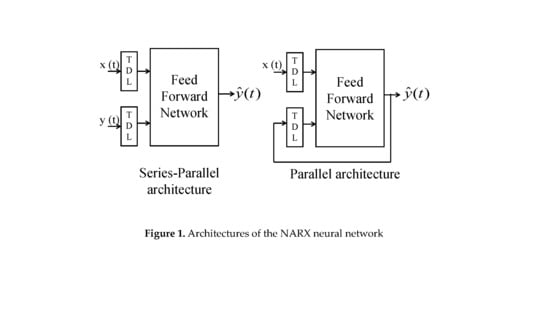
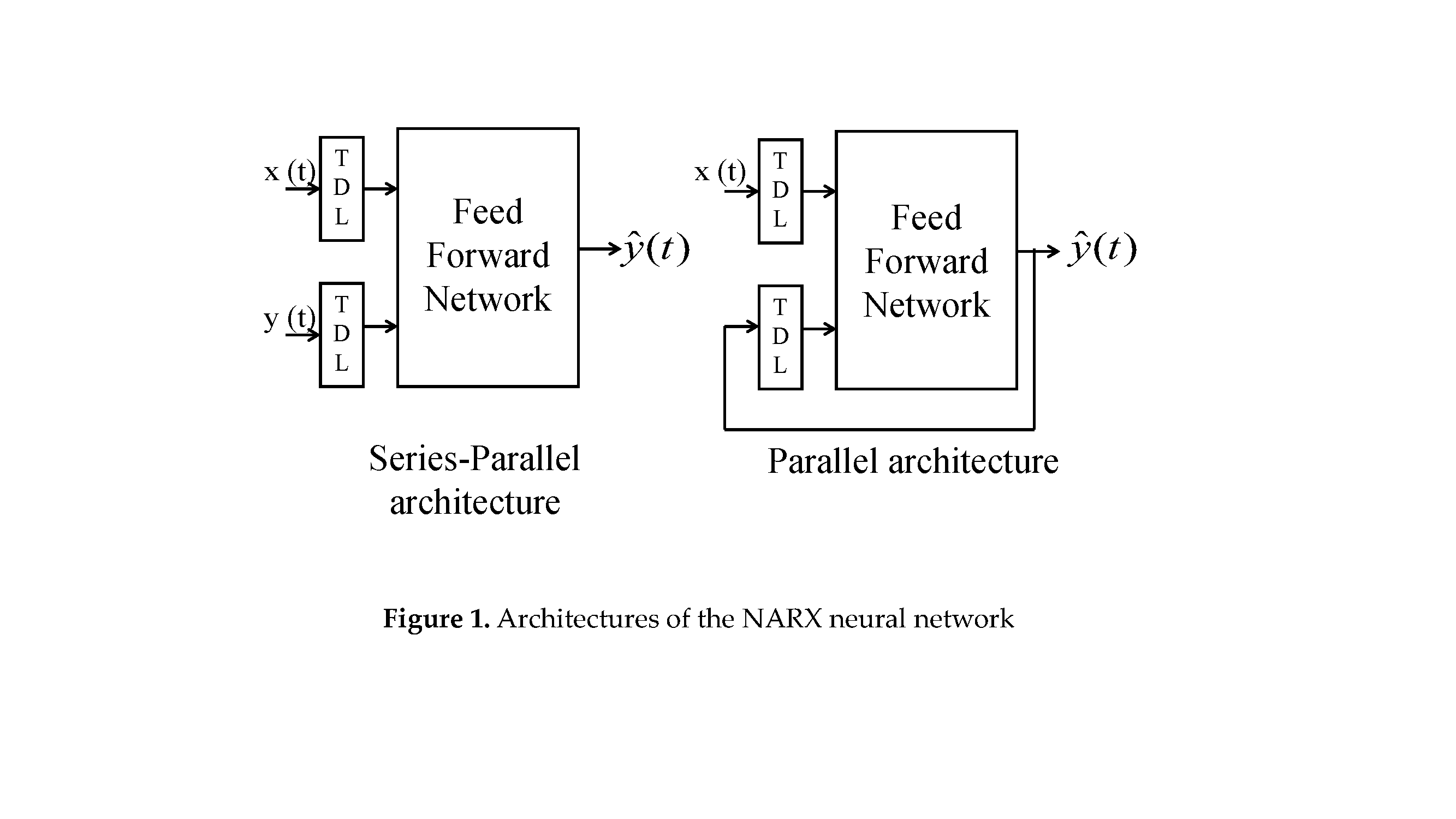
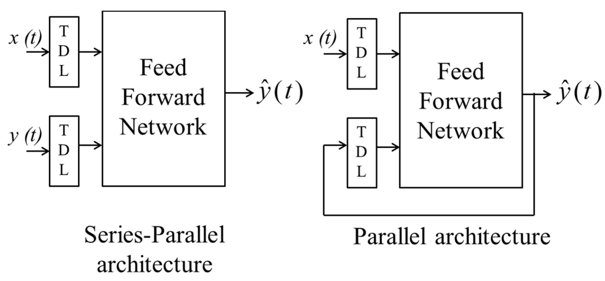
2. Artificial Neural Networks and NARX Model
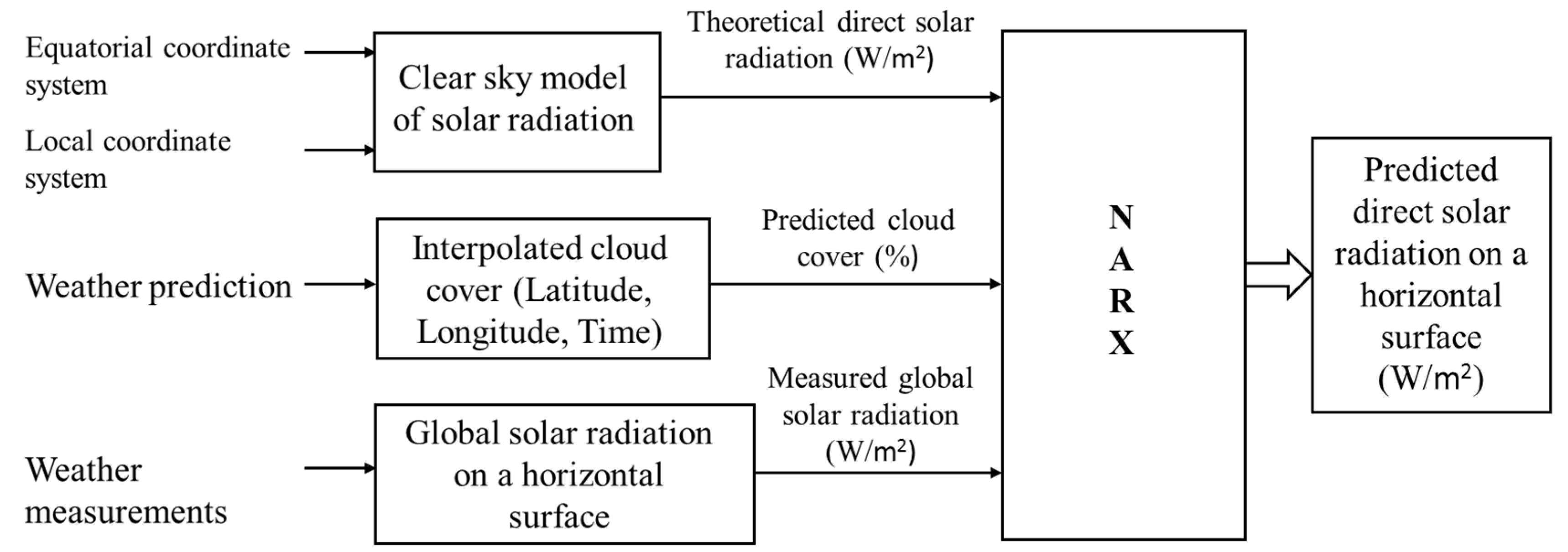
3. Model Structure and Used Database
- The deterministic component: it is the endogenous input of the NARX model. It is described mathematically by the clear sky model of the direct solar radiation. The clear sky model is calculated based on two coordinate systems: the equatorial coordinate system and the local coordinate system. The calculations are presented in Section 4.
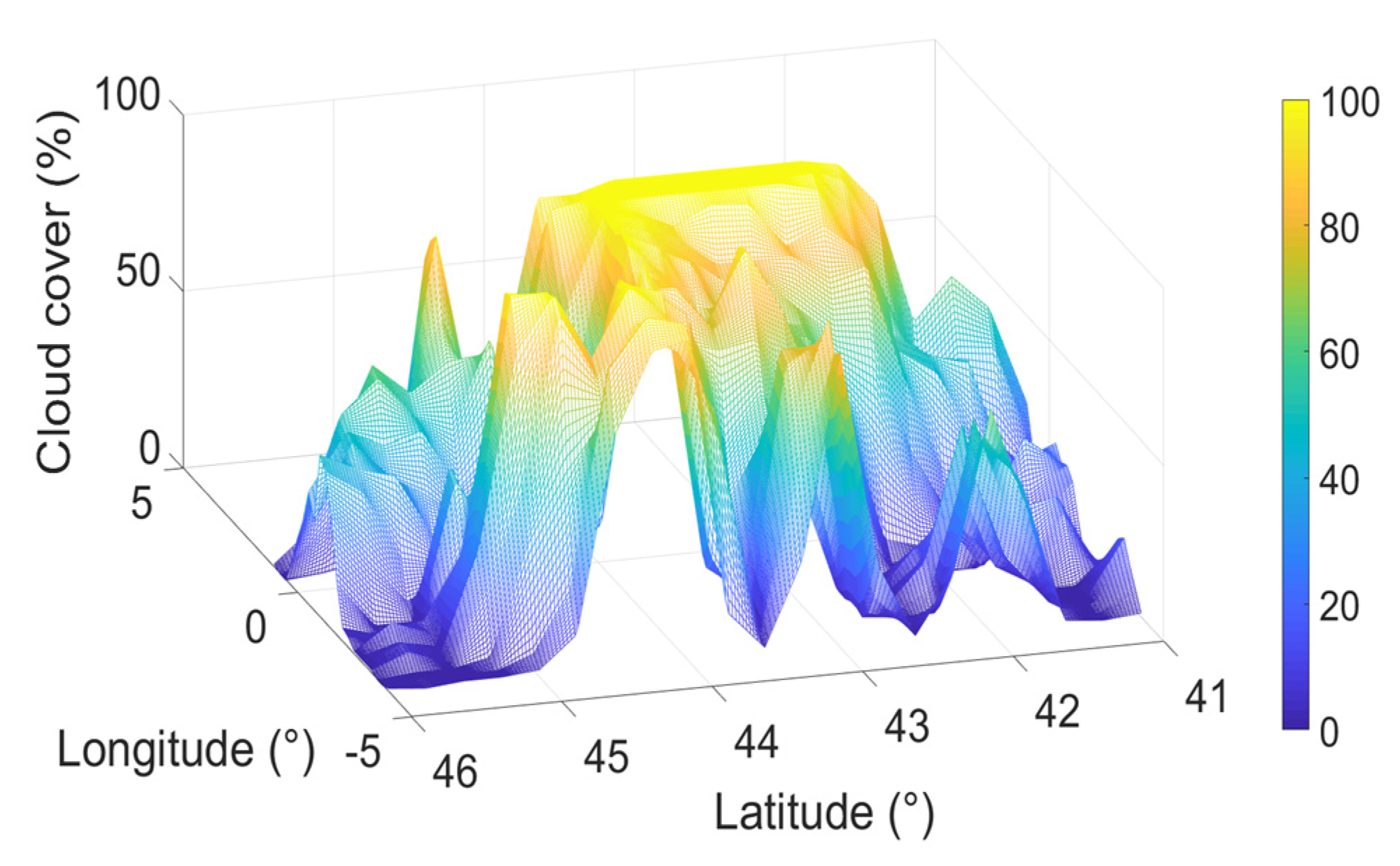
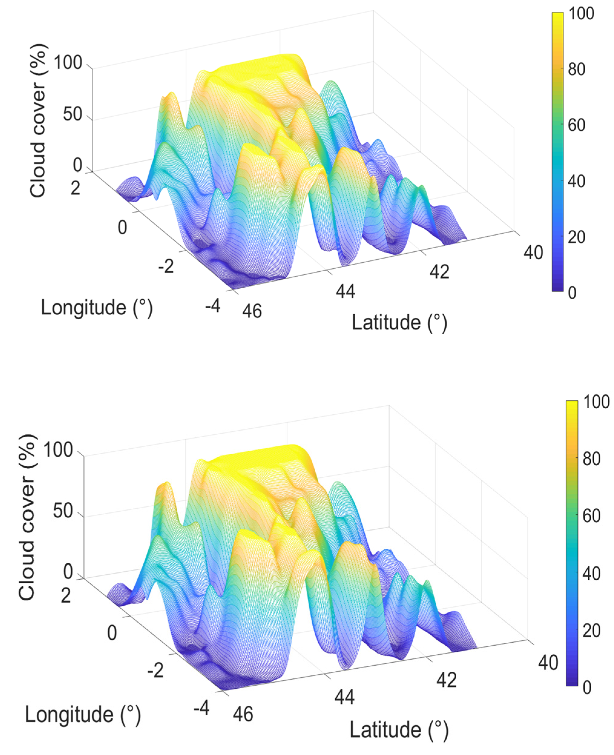
- The statistical component: is the exogenous input of the NARX model. Here, it contains only the cloud cover, because two reasons. First, the cloud cover is the most influential parameter on the direct solar radiation. Second, the identification of the other parameters is complicated. The construction of the cloud cover vector is presented in Section 5.
4. The Deterministic Component of the Direct Solar Radiation
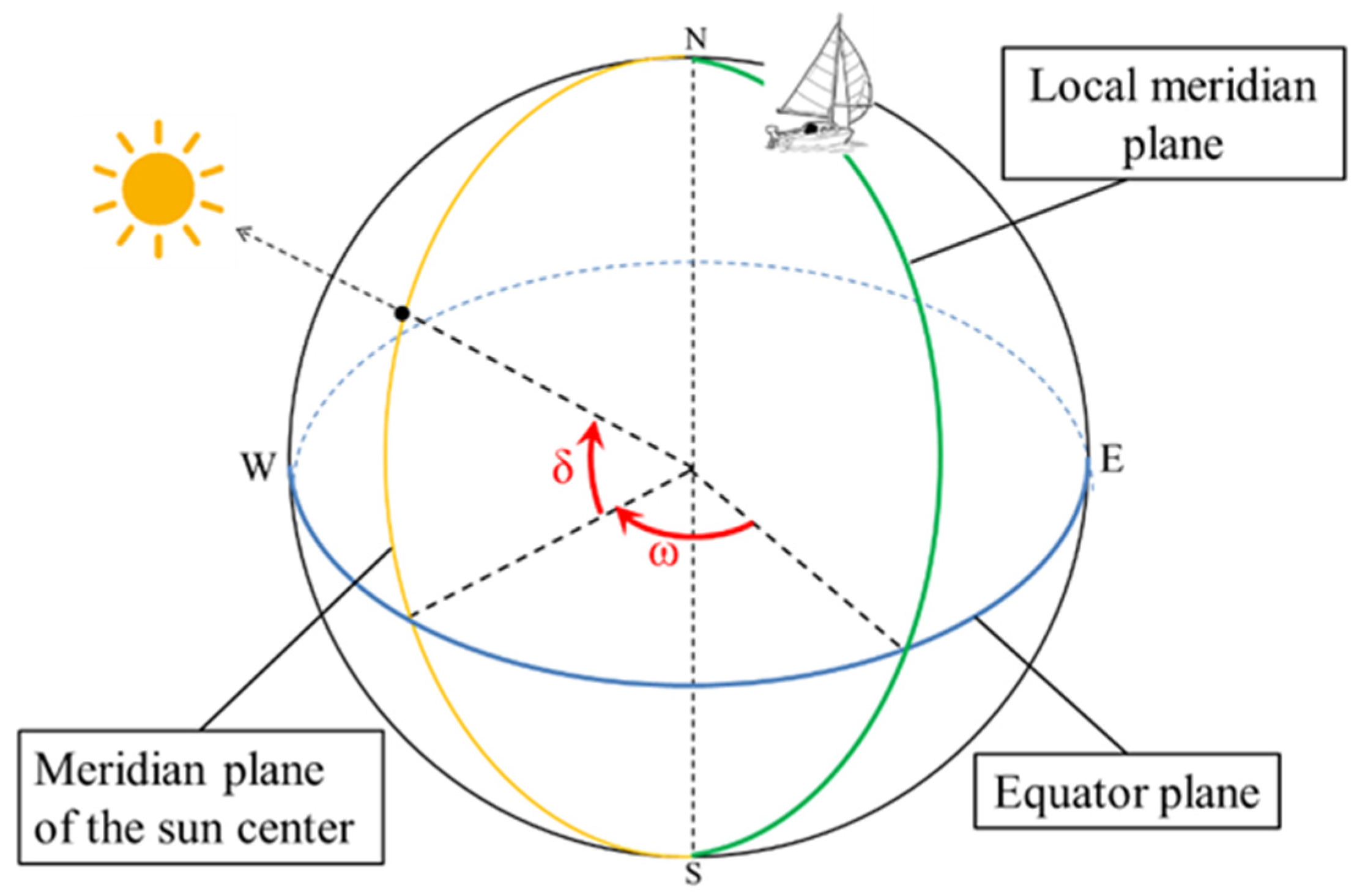
4.1. Calculation of the Geometrical Parameters
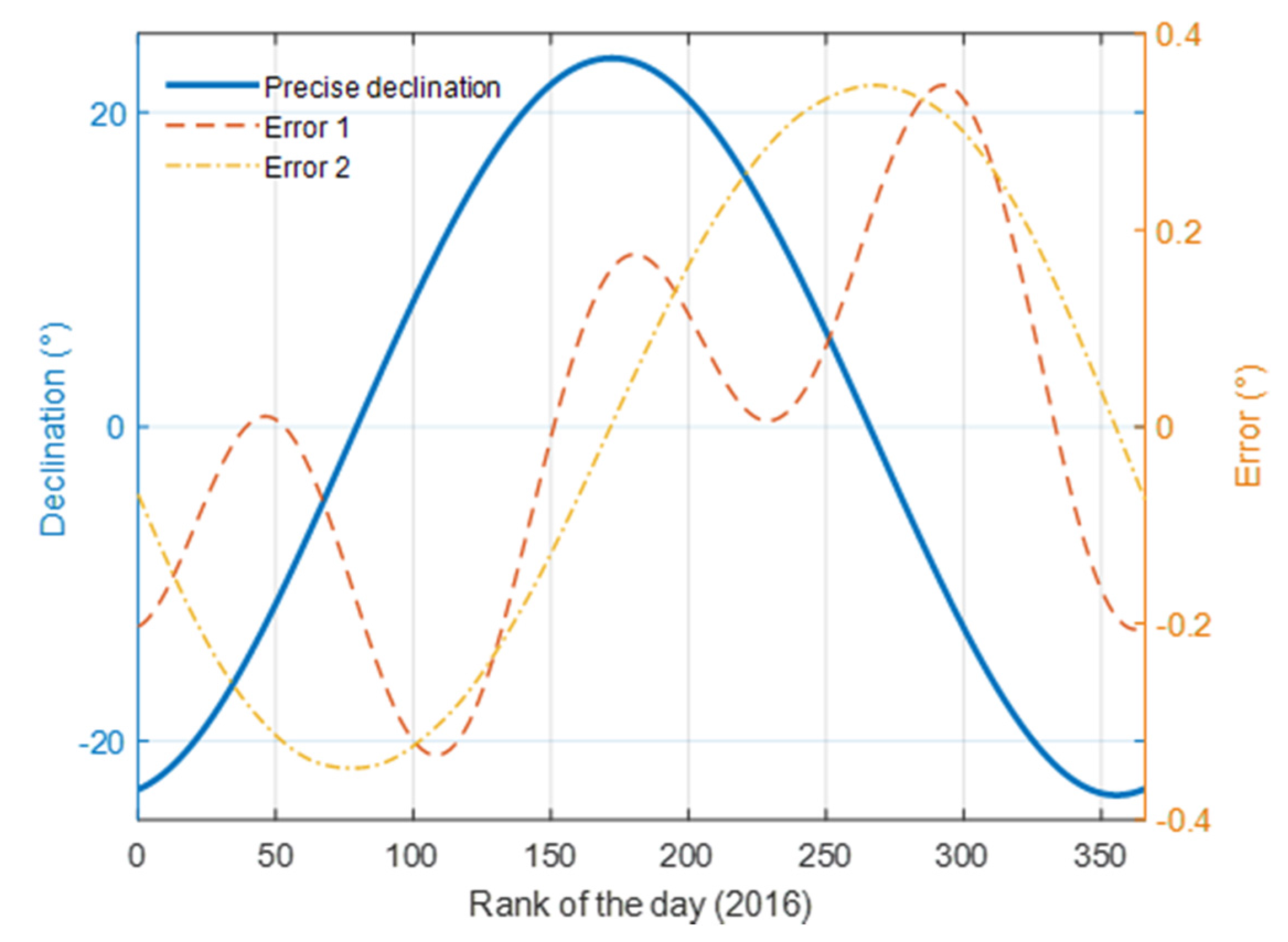
4.1.1. Sun’s Declination
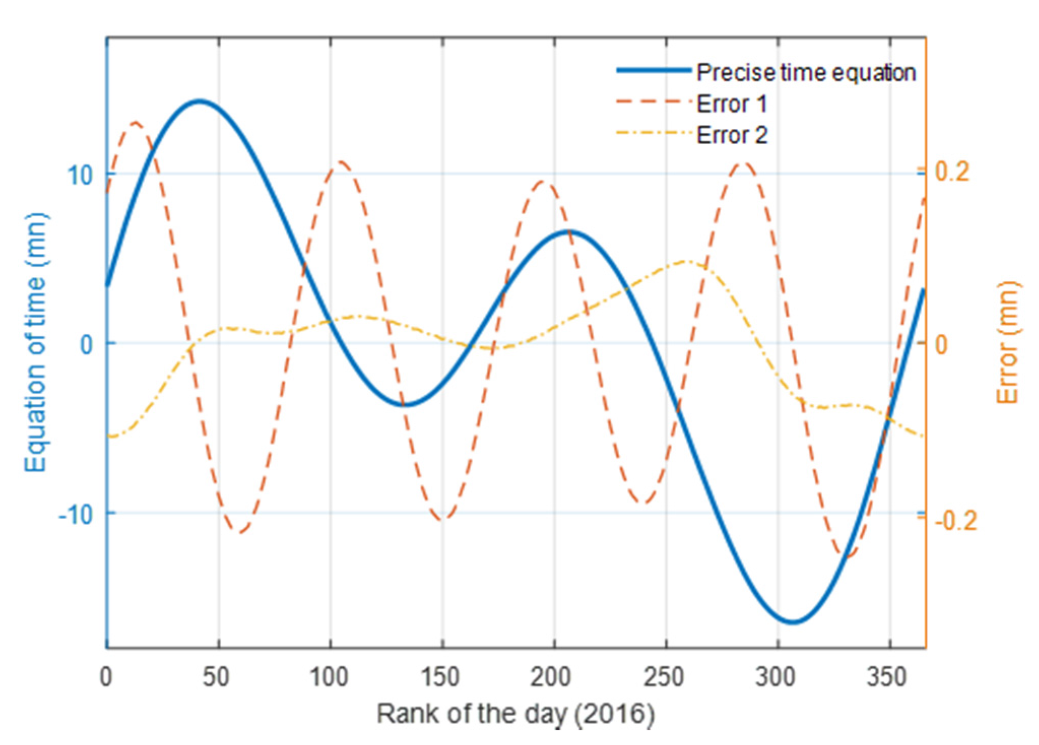
4.1.2. Equation of Time
4.1.3. Local and Solar Time
4.1.4. Hour Angle
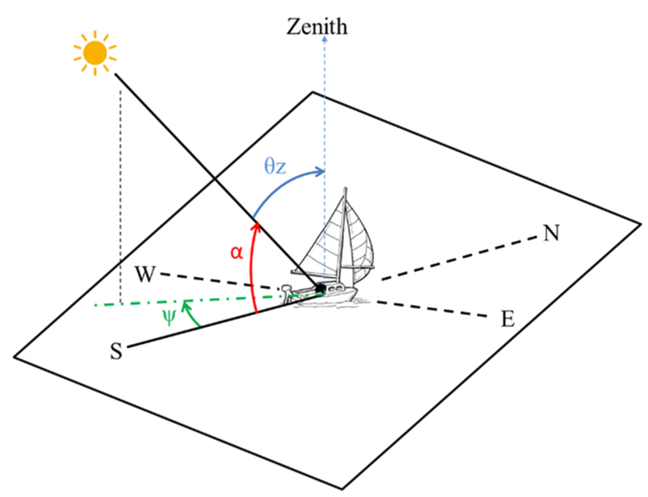
4.1.5. Sun Height
4.1.6. Azimuth Angle
4.1.7. Solar Radiation at the Top of Atmosphere
4.2. The Direct Solar Radiation Model
5. Interpolation of Downloaded Data
5.1. Geographical Interpolation
5.2. Time Interpolation
6. Adjustments, Results and Discussion
6.1. Evaluation Criteria
6.2. Results and Discussion
6.2.1. Choice of the Dataset Structure
- The meteorological conditions influencing the cloud cover variations.
- The localization influencing the direct solar radiation model variations, especially as in this study the localization data (longitude and latitude) are intercalated in a preliminary calculation (the SOLIS model) and not as inputs of the neural network.
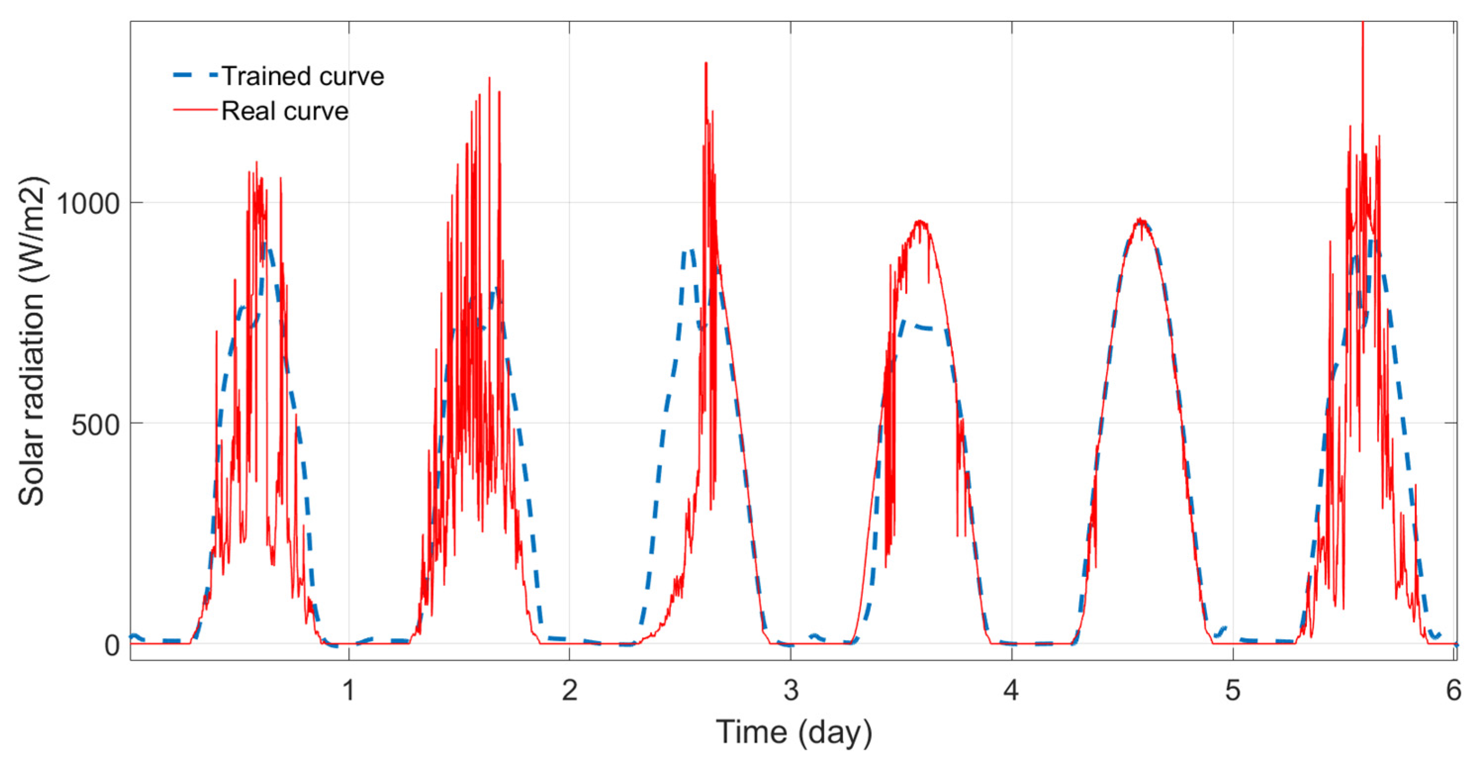
6.2.2. Choice of the Neural Network Structure
- The weights and biases vectors are randomly generated only once, in the first training phase. Then, in the following periodic training phases, the same weights and biases values are used.
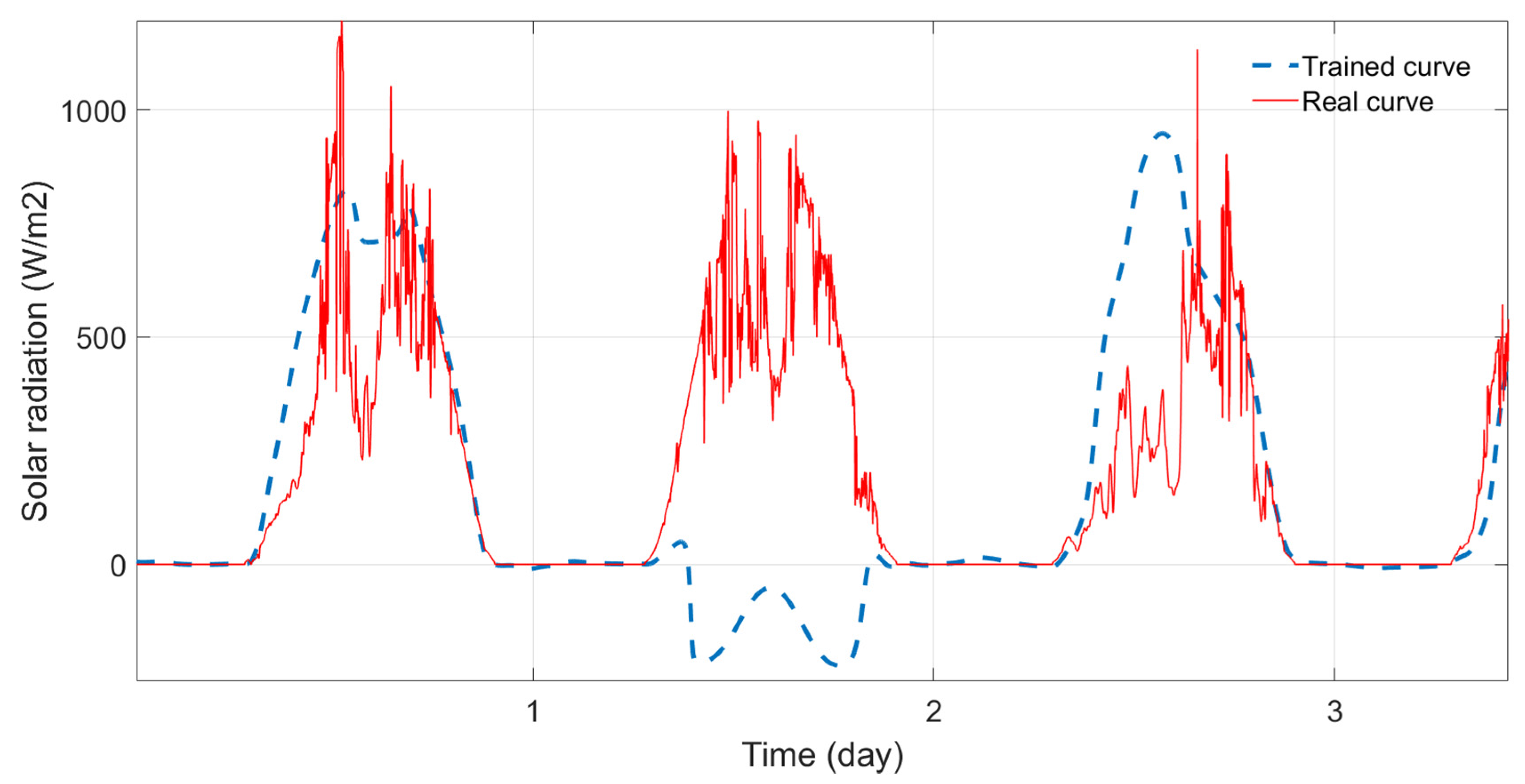
- Weights and biases are randomly initialized by ANN in each periodic training phase.
7. Conclusions
Author Contributions
Conflicts of Interest
Nomenclature
| C | Equation of the center (°) |
| cc | Time difference comparing to Greenwich (h) |
| e | Eccentricity of the ellipse e = 0.1671 |
| E | Equation of time (mn) |
| Esc | Solar constant (=1367 W/m2) |
| G | Direct solar radiation (W/m2) |
| G0 | Top-of-atmosphere solar radiation (W/m2) |
| N | Rank of the day (1 for 1 January 2013) |
| J | Rank day in the current year (1 for 1 January) |
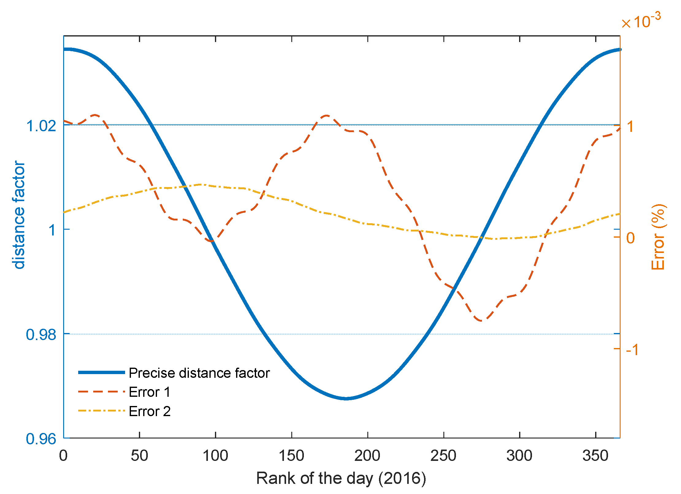
| KD | Distance correction factor Earth-Sun |
| L | Ecliptic longitude of the Sun (°) |
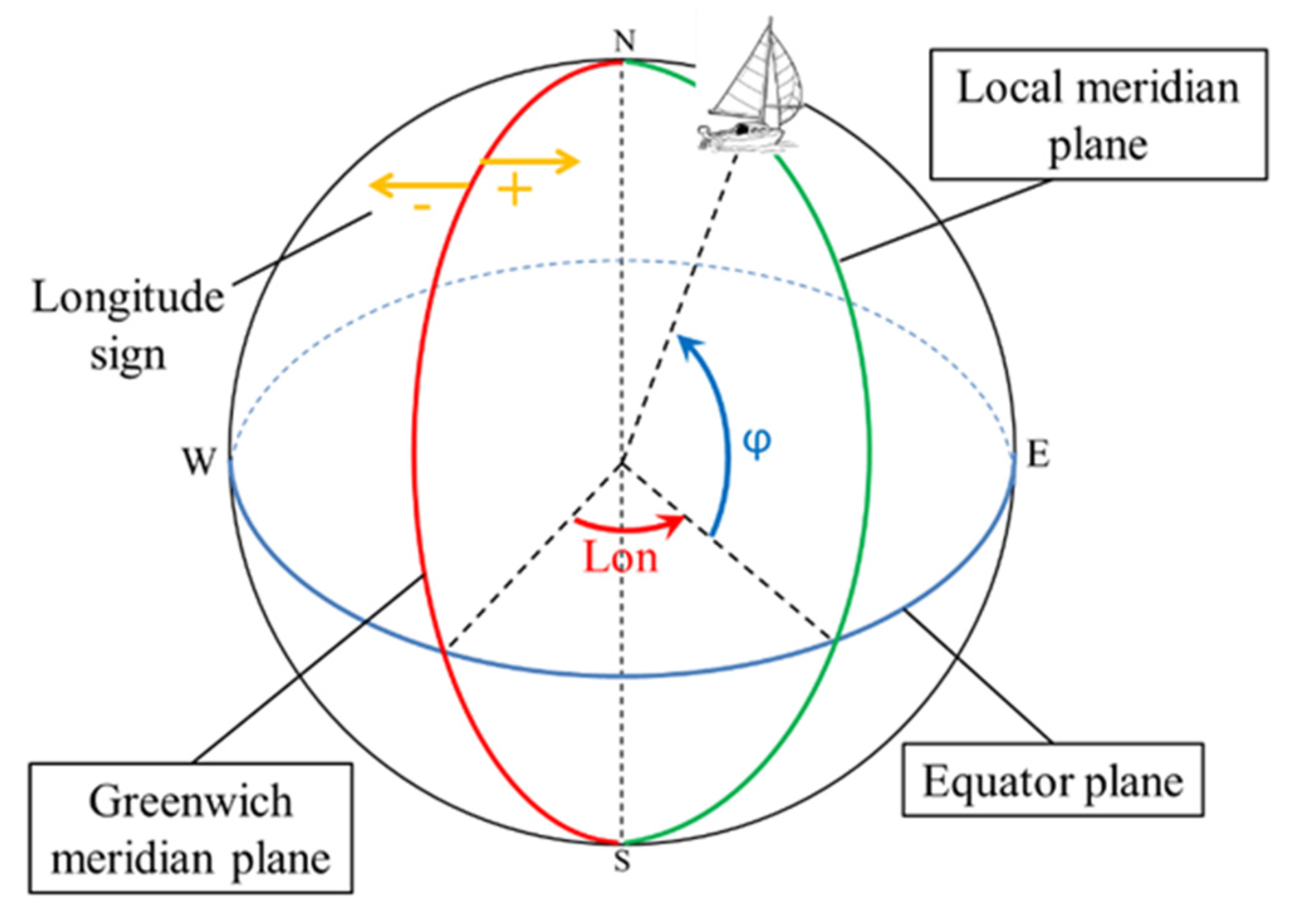
| Lon | Longitude (°) |
| Ma | Mean anomaly (°) |
| R | influence of obliquity (°) |
| R(J) | mean earth-Sun distance for the day J (au) |
| Rm | mean earth-Sun distance (au) |
| TCF | Local time (h) |
| TS | Solar time (h) |
| ϕ | Latitude (°) |
| δ | Sun’s declination (°) |
| ϖ | hour angle (°) |
| α | Sun height (°) |
| ψ | Solar azimuth angle (°) |
| θz | Zenith angle (°) |
| τ | Atmospheric optical depth |
| γ | Azimuth angle (°) |
References
- Zhang, W.-Y.; Zhao, Z.-B.; Han, T.T.; Kong, L.B. Short Term Wind Speed Forecasting for Wind Farms Using an Improved Auto regression Method. In Proceedings of the International Conference of Information Technology, Computer Engineering and Management Sciences, Nanjing, China, 24–25 September 2011. [Google Scholar]
- Wang, Z.; Tian, C.; Zhu, Q.; Huang, M. Hourly Solar Radiation Forecasting Using a Volterra-Least Squares Support Vector Machine Model Combined with Signal Decomposition. Energies 2018, 11, 68. [Google Scholar] [CrossRef]
- Voyant, C.; Muselli, M.; Paoli, C.; Nivet, M. Optimization of an artificial neural network dedicated to the multivariate forecasting of daily global radiation. Energy 2011, 36, 348–359. [Google Scholar] [CrossRef]
- Mohanty, S.; Patra, P.K.; Sahoo, S.S. Prediction of global solar radiation using nonlinear autoregressive network win exogenous inputs (narx). In Proceedings of the 39th National System Conference (NSC), Noida, India, 14–16 December 2015. [Google Scholar]
- Assas, O.; Bouzgou, H.; Fetah, S.; Salmi, M.; Boursas, A. Use of the artificial neural network and meteorological data for predicting daily global solar radiation in Djelfa, Algeria. In Proceedings of the International Conference on Composite Materials & Renewable Energy Applications (ICCMREA), Sousse, Tunisia, 22–24 January 2014. [Google Scholar]
- Nazaripouya, H.; Wang, B.; Wang, Y.; Chu, P.; Pota, H.R.; Gadh, R. Univariate time series prediction of solar power using a hybrid wavelet-ARMA-NARX Prediction Method. In Proceedings of the IEEE/PES Transmission and Distribution Conference and Exposition (T&D), Dallas, TX, USA, 3–5 May 2016. [Google Scholar]
- Wei, C.C. Predictions of surface solar radiation on tilted solar panels using machine learning models: Case study of Tainan City, Taiwan. Energies 2017, 10, 1660. [Google Scholar] [CrossRef]
- Cao, J.; Lin, X. Application of the diagonal recurrent wavelet neural network to solar irradiation forecast assisted with fuzzy technique. Eng. Appl. Artif. Intell. 2008, 21, 1255–1263. [Google Scholar] [CrossRef]
- Iqbal, M. An Introduction to Solar Radiation, 1st ed.; Elsevier: Amsterdam, The Netherlands, 1983. [Google Scholar]
- Jakhrani, A.Q.; Othman, A.K.; Rigit, A.R.H.; Samo, S.R.; Ling, L.P.; Baini, R. Evaluation of Incident Solar Radiation on Inclined Plane by Empirical Models at Kuching, Sarawak, Malaysia. In Proceedings of the International Conference on Renewable Energies and Power Quality—ICREPQ, Granada, Spain, 23–25 March 2010. [Google Scholar]
- Hoang, P.; Bourdin, V.; Liu, Q.; Caruso, G.; Archambault, V. Coupling optical and thermal models to accurately predict PV panel electricity production. Sol. Energy Mater. Sol. Cells 2014, 125, 325–338. [Google Scholar] [CrossRef]
- Duffie, J.A.; Beckman, W.A. Solar Engineering of Thermal Processes, 4th ed.; Wiley: Hoboken, NJ, USA, 2013. [Google Scholar]
- L’équation du Temps. Available online: http://kaekoda.free.fr/bup/bup2_html/bup2_htmlse2.html (accessed on 17 January 2018).
- L’énergie Solaire. Available online: http://herve.silve.pagesperso-orange.fr/solaire.htm (accessed on 17 January 2018).
- Calcul Simplifié des Valeurs de L’Equation du Temps et de la Déclinaison Solaire. Available online: http://jean-paul.cornec.pagesperso-orange.fr/equation.htm#_calcul (accessed on 17 January 2018).
- Heures des Lever et Coucher du Soleil Ephémérides de la Lune. Available online: http://jean-paul.cornec.pagesperso-orange.fr/heures_lc.htm (accessed on 17 January 2018).
- Benkaciali, S.; Gairaa, K. Modélisation de l’irradiation solaire globale incidente sur un plan incliné. Rev. Energies Renouv. 2014, 17, 245–252. [Google Scholar]
- Kerkouche, K.; Cherfa, F.; Hadj Arab, A.; Bouchakour, S.; Abdeladim, K.; Bergheul, K. Evaluation de l’irradiation solaire globale sur une surface inclinée selon differents modèles pour le site de Bouzaréah. Revue Energies Renouv. 2013, 16, 269–284. [Google Scholar]
- Yettou, F.; Malek, A.; Haddadi, M.; Gama, A. Etude comparative de deux modèles de calcul du rayonnement solaire par ciel clair en Algérie. Rev. Energies Renouv. 2009, 12, 331–346. [Google Scholar]
- Mellit, A.; Kalogirou, S.; Shaari, S.; Salhi, H.; Hadj Arab, A. Methodology for predicting sequences of mean monthly clearness index and daily solar radiation data in remote areas: Application for sizing a stand-alone PV system. Renew. Energy 2008, 33, 1570–1590. [Google Scholar] [CrossRef]
- Voyant, C. Prédiction de Séries Temporelles de Rayonnement Solaire Global et de Production D’énergie Photovoltaïque à Partir de Réseaux de Neurones Artificiels. Ph.D. Thesis, Universite de Corse-Pascal Paoli Ecole Doctorale Environnement et Societe Umr Cnrs 6134 (SPE), Corte, France, 6 November 2011. [Google Scholar]
- Ineichen, P. Comparison of eight clear sky broadband models against 16 independent data banks. Sol. Energy 2006, 80, 468–478. [Google Scholar] [CrossRef]
- Pisoni, E.; Farina, M.; Carnevale, C.; Piroddi, L. Forecasting peak air pollution levels using NARX models. Eng. Appl. Artif. Intell. 2009, 22, 593–602. [Google Scholar] [CrossRef]
- Ruiz, L.G.B.; Cuéllar, M.P.; Calvo-Flores, M.D.; Jiménez, M.D.C.P. An Application of Non-Linear Autoregressive Neural Networks to Predict Energy Consumption in Public Buildings. Energies 2016, 9, 684. [Google Scholar] [CrossRef]
- Araújo, R.A.; Oliveira, A.L.I.; Meira, S. A morphological neural network for binary classification problems. Eng. Appl. Artif. Intell. 2017, 65, 12–28. [Google Scholar] [CrossRef]
- Gong, T.; Fan, T.; Guo, J.; Cai, Z. GPU-based parallel optimization of immune convolutional neural network and embedded system. Eng. Appl. Artif. Intell. 2017, 62, 384–395. [Google Scholar] [CrossRef]
- Sánchez, D.; Melin, P.; Castillo, O. Optimization of modular granular neural networks using a firefly algorithm for human recognition. Eng. Appl. Artif. Intell. 2017, 64, 172–186. [Google Scholar] [CrossRef]
- Yu, S.; Zhu, K.; Zhang, X. Energy demand projection of China using a path-coefficient analysis and PSO–GA approach. Energy Conver. Manag. 2012, 53, 142–153. [Google Scholar] [CrossRef]
- Chen, S.; Billings, S.; Grant, P. Non-linear system identification using neural networks. Int. J. Control 1990, 51, 1191–1214. [Google Scholar] [CrossRef]
- Cadenas, E.; Rivera, W.; Campos-Amezcua, R.; Heard, C. Wind Speed Prediction Using a Univariate ARIMA Model and a Multivariate NARX Model. Energies 2016, 9, 109. [Google Scholar] [CrossRef]
- Ferreira, A.A.; Ludermir, T.B.; Aquino, R. Comparing recurrent networks for time-series forecasting. In Proceedings of the 2012 International Joint Conference on Neural Networks (IJCNN), Brisbane, Australia, 10–15 Junuary 2012. [Google Scholar]
- Buitrago, J.; Asfour, S. Short-Term Forecasting of Electric Loads Using Nonlinear Autoregressive Artificial Neural Networks with Exogenous Vector Inputs. Energies 2017, 10, 40. [Google Scholar] [CrossRef]
- Ali, M.H. Fundamentals of Irrigation and On-Farm Water Management; Springer: Berlin, Germany, 2010; Volume 1, ISBN 978-1-4419-6335-2. [Google Scholar]
- Ephemeride Generator of Institut de Mecanique Celeste et de Calcul des Ephemerides. Available online: http://www.imcce.fr/langues/fr/ephemerides/generateur_ephemerides.html (accessed on 18 January 2018).
- Influence de L’ellipticité de la Trajectoire. Available online: http://kaekoda.free.fr/bup/bup2_html/bup2_htmlse2.html (accessed on 18 January 2018).
- Du Temps Solaire au Temps Légal, Equation du Temps. Available online: http://jean-paul.cornec.pagesperso-orange.fr/equation.htm#_calcul (accessed on 18 January 2018).
- Astronomie—Sphère Céleste, Mouvement du Soleil, Mouvement du Soleil sur la Sphère Céleste. Available online: https://sites.google.com/site/astronomievouteceleste/4---mouvement-du-soleil (accessed on 18 January 2018).
- Cox, A. Allen’s Astrophysical Quantities, 4th ed.; Springer: Berlin, Germany, 2002. [Google Scholar]
- Guide des Données Astronomiques (Annuaire du Bureau des Longitudes); EDP Sciences: Les Ulis, France, 2016.
- Oumbe Ndeffotsing, A.B. Exploitation des Nouvelles Capacités D’observation de la Terre Pour Evaluer le Rayonnement Solaire Incident au Sol. Ph.D. Thesis, Ecole Nationale Supérieure des Mines de Paris, Paris, France, 9 November 2009. [Google Scholar]
- Danel, K.; Gautret, L. Génération du Disque Solaire des Communes de L’Ouest; ARER: Paris, France, 2008. [Google Scholar]
- Chassagne, G.; Dupuy, C.; Levy, M. Énergie Solaire—Conversion et Applications; CNRS: Paris, France, 1978; pp. 135–170. [Google Scholar]
- Sleiman, W.; Matta, E.; Saleh, C. Hybrid Rural Mini Electric Grid. Ph.D. Thesis, Lebanese University, Beirut, Lebanon, 29 July 2013. [Google Scholar]
- Atmospheric Science Data Center. Available online: https://eosweb.larc.nasa.gov (accessed on 18 January 2018).
- Aguiar, R.J.; Collares-Pereira, M.; Conde, J.P. Simple procedure for generating sequences of daily radiation values using a library of Markov transition matrices. Sol. Energy 1988, 40, 269–279. [Google Scholar] [CrossRef]
- Matthew, J.R.; Clifford, W.H.; Joshua, S.S. Global Horizontal Irradiance Clear Sky Models: Implementation and Analysis; Sandia Report Sand 2012-2389; Sandia National Laboratories: Livermore, CA, USA, 2012.
- Lefevre, M.; Oumbe, A.; Blanc, P.; Espinar, B.; Gschwind, B.; Qu, Z.; Wald, L.; Schroedter-Homscheidt, M.; Hoyer-Klick, C.; Arola, A.; et al. McClear: A new model estimating downwelling solar radiation at ground level in clear-sky conditions. Atmos. Measure. Tech. Eur. Geosci. Union 2013, 6, 2403–2418. [Google Scholar] [CrossRef] [Green Version]
- Ineichen, P.; Guisan, O.; Perez, R. Ground-reflected radiation and albedo. Sol. Energy 1990, 44, 207–214. [Google Scholar] [CrossRef]
- Kasten, F. The linke turbidity factor based on improved values of the integral Rayleigh optical thickness. Sol. Energy 1996, 56, 239–244. [Google Scholar] [CrossRef]
- Molineaux, B.; Ineichen, P.; O’Neill, N. Equivalence of Pyrheliometric and Monochromatic Aerosol Optical Depths at a Single Key Wavelength. Appl. Opt. 1998, 37, 7008–7018. [Google Scholar] [CrossRef] [PubMed]
- Mueller, R.W.; Dagestad, K.F.; Ineichen, P.; Schroedter-Homscheidt, M.; Cros, S.; Dumortier, D.; Kuhlemann, R.; Olseth, J.; Piernavieja, G.; Reise, C.; et al. Rethinking satellite-based solar irradiance modelling: The SOLIS clear-sky module. Remote Sens. Environ. 2004, 91, 160–174. [Google Scholar] [CrossRef]
- Ineichen, P. A broadband simplified version of the SOLIS clear sky model. Sol. Energy 2008, 82, 758–762. [Google Scholar] [CrossRef]
- Agarwal, R.P.; Wong, P.J.Y. Error Inequalities in Polynomial Interpolation and Their Applications, Chapter 5. In Piecewise—Polynomial Interpolation; Springer: Berlin, Germany, 1993; Volume 262, pp. 217–280. ISBN 978-94-010-4896-5. [Google Scholar]
- Iwashita, Y. OpenGamma Quantitative Research, Piecewise Polynomial Interpolations. 2013. Available online: https://developers.opengamma.com/quantitative-research/Piecewise-Polynomial-Interpolation-OpenGamma.pdf (accessed on 9 March 2018).
- Karlik, B.; Vehbi, A. Performance Analysis of Various Activation Functions in Generalized MLP Architectures of Neural Networks. Int. J. Artif. Intell. Exp. Syst. 2011, 1, 111–122. [Google Scholar]


| Function | Definition | Codomain |
|---|---|---|
| Linear | x | The Real domain IR |
| Sigmoid (Logsig) | ]0, 1[ | |
| Hyperbolic tangent (Tansig) | ]-1, 1[ |
| Database Size | MSE | DMPE (W/m2) |
|---|---|---|
| 5 days | 0.011 | 60.228825 |
| 10 days | 0.00695 | 41.19645 |
| 15 days | 0.009625 | 50.2089 |
| Time Average | MSE | DMPE (W/m2) |
|---|---|---|
| 10 min | 0.00732 | 44.4344 |
| 30 min | 0.00695 | 41.19645 |
| Property | Choice |
|---|---|
| Number of hidden layers | 1 |
| Normalization Interval of dataset | [0.05, 0.95] |
| Delay vectors | Input data: [0, 1] Target: [1, 2] |
| Training parameters | Error: MSE Learning algorithm: Levenberg-Marquardt |
| Number of Neurons | MSE | DMPE (W/m2) |
|---|---|---|
| 10 × 10 × 1 | 0.00724 | 59.5724 |
| 15 × 15 × 1 | 0.00410 | 30.4164 |
| 16 × 16 × 1 | 0.01438 | 73.4646 |
| 20 × 20 × 1 | 0.00768 | 45.0513 |
| 22 × 22 × 1 | 0.00695 | 41.1964 |
| Generation of Weights | MSE | DMPE (W/m2) |
|---|---|---|
| Initialized | 0.00410 | 30.4164 |
| Random | 0.00279 | 24.0584 |
© 2018 by the authors. Licensee MDPI, Basel, Switzerland. This article is an open access article distributed under the terms and conditions of the Creative Commons Attribution (CC BY) license (http://creativecommons.org/licenses/by/4.0/).
Share and Cite
Boussaada, Z.; Curea, O.; Remaci, A.; Camblong, H.; Mrabet Bellaaj, N. A Nonlinear Autoregressive Exogenous (NARX) Neural Network Model for the Prediction of the Daily Direct Solar Radiation. Energies 2018, 11, 620. https://doi.org/10.3390/en11030620
Boussaada Z, Curea O, Remaci A, Camblong H, Mrabet Bellaaj N. A Nonlinear Autoregressive Exogenous (NARX) Neural Network Model for the Prediction of the Daily Direct Solar Radiation. Energies. 2018; 11(3):620. https://doi.org/10.3390/en11030620
Chicago/Turabian StyleBoussaada, Zina, Octavian Curea, Ahmed Remaci, Haritza Camblong, and Najiba Mrabet Bellaaj. 2018. "A Nonlinear Autoregressive Exogenous (NARX) Neural Network Model for the Prediction of the Daily Direct Solar Radiation" Energies 11, no. 3: 620. https://doi.org/10.3390/en11030620