Explicit Multipole Formulas for Calculating Thermal Resistance of Single U-Tube Ground Heat Exchangers †


1
Building Physics, Lund University, Lund 221 00, Sweden
2
Building Services Engineering, Chalmers Technical University, Gothenburg 412 96, Sweden
*
Author to whom correspondence should be addressed.
†
Presented at the IGSHPA Technical/Research Conference and Expo, Denver, CO, USA, 14–16 March 2017.
Energies 2018, 11(1), 214; https://doi.org/10.3390/en11010214
Submission received: 30 November 2017
/
Revised: 10 January 2018
/
Accepted: 10 January 2018
/
Published: 16 January 2018
(This article belongs to the Special Issue Geothermal Heating and Cooling)
Abstract
:Borehole thermal resistance is both an important design parameter and a key performance characteristic of a ground heat exchanger. Another quantity that is particularly important for ground heat exchangers is the internal thermal resistance between the heat exchanger pipes. Both these resistances can be calculated to a high degree of accuracy by means of the well-known multipole method. However, the multipole method has a fairly intricate mathematical algorithm and is thus not trivial to implement. Consequently, there is considerable interest in developing explicit formulas for calculating borehole resistances. This paper presents derivation and solutions of newly derived second-order and higher-order multipole formulas for calculating borehole thermal resistance and total internal thermal resistance of single U-tube ground heat exchangers. A new and simple form of the first-order multipole formula is also presented. The accuracy of the presented formulas is established by comparing them to the original multipole method. The superiority of the new higher-order multipole formulas over the existing formulas is also demonstrated.
1. Introduction
The use of ground source heat pump (GSHP) systems to provide heating and cooling in buildings has increased at a rapid rate in the last two decades or so. Stimulated by energy prices, technology advances and environmental concerns, the thermal energy utilized by these systems has increased from approximately 500 GWh in 1995 to over 91,000 GWh in 2015. During the same period, the worldwide installed capacities of these systems have increased from under 2000 MWt in 1995 to over 50,000 MWt in 2015 [1]. Comparable growth levels are expected for the future.
A typical GSHP system consists of a heat pump, a ground heat exchanger, and auxiliary systems for storage and distribution of thermal energy. The sizing and performance of a heat pump system depends upon the coefficient of performance of the heat pump, which in turn is a function of heat source and heat sink temperatures. Compared to ambient air, ground, in general, is a far superior source or sink of thermal energy because of its relatively stable temperature levels over the year. In a GSHP system, a ground heat exchanger is used to transfer heat to or from the ground. The ground heat exchanger can be of open or closed type. In an open system groundwater is directly used as the heat carrier fluid, whereas in a closed system the heat carrier fluid is circulated in a closed loop, which can be horizontal or vertical. Various heat exchanger configurations can be used in closed-loop vertical systems, including single or double U-tubes, and simple or complex coaxial pipes. Among all types, a borehole heat exchanger with a single U-tube is by far the most commonly used ground heat exchanger in practice because of its low cost, small space requirements, and ease of installation. The scope of this paper is also limited to the application of single U-tubes in borehole heat exchangers.
Ground thermal conductivity (λ) and borehole thermal resistance (Rb) are the two principal parameters that govern the heat transfer mechanism of a borehole heat exchanger, and thus influence the sizing and performance of the overall GSHP system [2]. The heat transfer outside the borehole boundary is dictated by the thermal conductivity of the ground, whereas the heat transfer inside the borehole is characterized by the borehole thermal resistance between the heat carrier fluid and the borehole wall. A high ground thermal conductivity is beneficial for the ground heat transfer. However, being an intrinsic property of the ground, ground thermal conductivity cannot be controlled in practice. On the other hand, a low borehole thermal resistance is desirable for better heat transfer inside the borehole heat exchanger. The borehole thermal resistance depends upon the physical arrangement and the thermal properties of borehole components including grouting, heat exchanger pipes, and the heat carrier fluid. Its value can be engineered to a certain extent by optimizing the geometry and layout of the borehole heat exchanger and by choosing appropriate materials for the borehole components.
For any given borehole configuration, the borehole thermal resistance can either be estimated theoretically [3] or measured experimentally [4]. The theoretical methods to estimate borehole thermal resistance include analytical [5,6,7] or empirical [8,9,10,11] formulas based on one-dimensional or two-dimensional steady-state conductive heat transfer in the borehole. As demonstrated by [12,13], there exists a great disparity between borehole thermal resistance values calculated from different theoretical methods. Many of the simplified methods work well in certain situations and poorly in others.
The multipole method is an analytical method to determine thermal resistances for any number of arbitrarily placed pipes in a composite region. It is based on two-dimensional steady-state conductive heat transfer in a borehole, and uses a combination of line heat sources and so-called multipoles to determine thermal resistances for any number of arbitrarily placed pipes in a composite region. The method was originally developed by [14,15], and was later revised by [16]. The main difference between the versions of [14] and [16] was in regards to prescribing a constant temperature condition at a suitable radial distance outside the borehole. In the later version, this condition was replaced by a condition on the mean temperature around the borehole wall, which simplified the algorithm.
The multipole method has been compared to and tested against several numerical methods. Young [17] compared the tenth-order multipole method with a boundary-fitted coordinates finite volume methods for 18 combinations of shank spacing and grout conductivities, and observed a maximum difference of 0.26% between the two methods. Lamarche et al. [12] calculated a root-mean-square difference of 0.003 between the first-order multipole method and a finite element numerical model for 72 studied cases with varying grout and soil conductivities, and pipe sizes and positing. He [18] studied four cases of different borehole diameters and grout conductivities using a three-dimensional numerical model and the multipole method, and reported a maximum difference of 0.19%. Liao et al. [11] compared the first-order multipole method with a two-dimensional numerical method and noted a maximum relative difference of 0.2% for 18 combinations of shank spacing and grout conductivities. Al-Chalabi [19] studied 12 different cases of pipe positioning, and grout and soil conductivities, using the first-order multipole method and a two-dimensional finite element method, and observed a maximum difference of 1.3% between the two methods.
The accuracy and the complexity of the multipole method increases with the number of multipoles used for the calculation. When implemented in a computer program, the order of the multipoles to be used for a calculation is typically prescribed to ten, which was the maximum possible order in the original implementation [14] of the multipole method. Popular ground heat exchanger programs Earth Energy Designer (EED, v3.2. BLOCON: Lund, Sweden) [20] and Ground Loop Heat Exchanger Professional (GLHEPro) [21] also use tenth-order multipoles when calculating the borehole thermal resistance. The tenth-order multipole calculations have an accuracy of over eight decimal digits [22].
On the adverse side, the actual multipole method has a quite rigorous mathematical formulation and a fairly complex algorithm. Its implementation in computer programs requires a considerable amount of coding (the original implementation [14] in FORTRAN was nearly 600 lines in length). However, it is possible to simplify the multipole method to explicit closed-form formulas assuming that heat exchanger pipes are placed symmetrically about the center of the borehole. In reality, heat exchanger pipes may be located anywhere in the borehole as long as they do not overlap each other. The position of pipes also varies along the depth of the borehole. However, in the absence of any a priori knowledge of the pipe positions, it is reasonable to assume that the heat exchanger pipes are symmetrically placed about the center of the borehole. So far, closed-form multipole formulas for zeroth-order and first-order have been developed for the case of a single U-tube with symmetrical pipes [23].
In this paper, we present derivation and solutions of new second-order and higher-order multipole formulas for calculating borehole thermal resistance of single U-tube ground heat exchangers with symmetric pipes. The presented formulas are tested against the original multipole method (i.e., the tenth-order multipole calculation) as well as previously-derived zeroth-order and first-order multipole formulas.
2. Borehole Thermal Resistance
The borehole thermal resistance (Rb) is the ratio of the temperature difference between the heat carrier fluid and the borehole wall to the heat transfer rate per unit length of the borehole. It is defined locally at a specific depth in the borehole as represented in Equation (1), where Tf,loc is the local mean fluid temperature, Tb is the average borehole wall temperature and qb is the heat transfer rate per unit length of the borehole.
Borehole thermal resistance is sometimes treated as a sum of resistances in series. The total borehole resistance (Rb) i.e., fluid-to-ground resistance is considered to be made up of two major parts: pipe resistance (Rp) and grout resistance (Rg). The pipe resistance includes both conductive resistance of the pipe (Rpc) and convective resistance of the fluid (Rpic). The grout resistance constitutes the thermal resistance between the outer pipe wall of the U-tube and the borehole wall. Its value depends on the pipe resistance and the ground thermal conductivity [13]. As the individual pipe resistances are in parallel with each other, the pipe resistance is generally calculated for a single pipe and is then divided by the total number (N) of pipes.
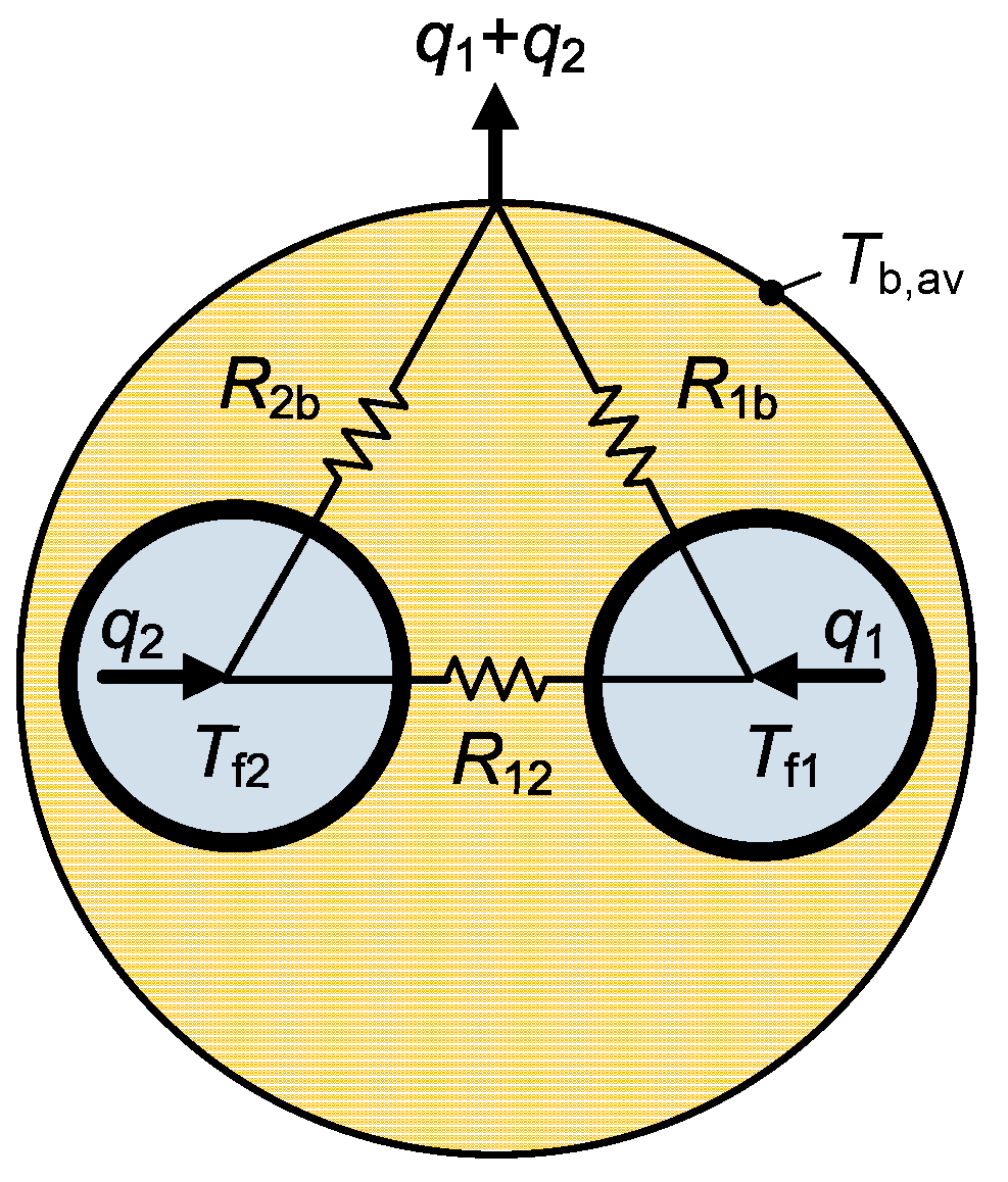
Nevertheless, in order to fully understand the concept of borehole thermal resistance, it is helpful to use a resistance network. Figure 1 shows an example of such a network for a single U-tube borehole. Other networks forms can also be formulated, e.g., see [11,24] but any such representation is an approximation to reality under network-specific assumptions and restrictions.
The three resistance Δ network of Figure 1 is based on the following relations between heat flows q1 and q2 and fluid temperatures Tf1 and Tf2.
In the above equations R1b and R2b are thermal resistances between pipe 1 or 2 and the borehole wall, respectively, and R12 is the fluid-to-fluid thermal resistance between pipes 1 and 2. These resistances include the thermal resistances of the fluid and the pipe. Using the Δ network of Figure 1, the total borehole resistance, Rb, can be determined by setting the fluid temperatures Tf1 = Tf2 and solving for two parallel resistances R1b and R2b:
The Δ network can also be used to determine resistance Ra by setting the heat flows q1 = −q2. The resistance, Ra, is the total internal resistance between the upward and downward flowing legs of the U-tube when there is no net heat flow from the borehole. It is related to the fluid-to-fluid internal resistance R12 by the thermal network of Figure 1. The resistance R12, which is sometimes also referred to as the direct coupling resistance, is the effect of the network representation and is not a directly measurable physical resistance. Resistance R12 is in parallel with the series resistances R1b and R2b.
The concept of total internal resistance Ra is critical to the understanding of the effective borehole thermal resistance , which is the thermal resistance between the heat carrier fluid, characterized by a simple mean Tf of the inlet and outlet temperatures, and the average borehole wall temperature Tb. The effective borehole thermal resistance is mathematically expressed as Equation (7).
The difference between borehole thermal resistance Rb, defined by Equation (1), and effective borehole thermal resistance , defined by Equation (7), is that the borehole thermal resistance applies locally at a specific depth in the borehole, whereas effective borehole thermal resistance applies to the entire borehole. The effective borehole thermal resistance is what is measured in an experiment, for example an in-situ thermal response test. The experimental measurements of mean fluid temperature taken at the top of the borehole include the effects of thermal short-circuiting between the upward and downward flows in the U-tube. Consequently, the effective borehole thermal resistance is often higher than the borehole thermal resistance due to the higher fluid temperature caused by the thermal short-circuiting between the U-tube pipes.
It is possible to calculate the effective borehole thermal resistance from the borehole thermal resistance [23,25,26]. Equations (8) and (9), developed by [23], are commonly used for this purpose. These equations correspond to two distinct boundary conditions of uniform borehole wall temperature and uniform heat flux along the borehole, respectively. Both these are limiting conditions and the real situation falls somewhere in between. Therefore, the effective borehole thermal resistance is commonly determined as the mean value between these two equations. Calculation of the effective borehole thermal resistance from Equations (8) and (9) requires knowledge of total internal thermal resistance Ra and direct coupling resistance R12 between the two U-tube legs, respectively, in addition to the borehole thermal resistance Rb.
3. Multipole Method for N Pipes in a Borehole
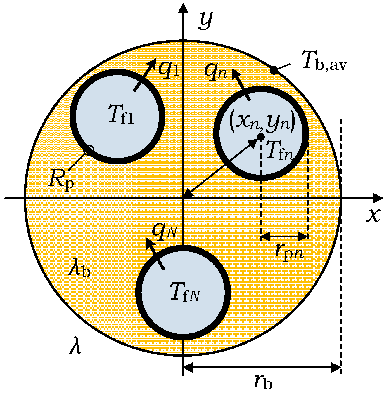
The general multipole method may be applied for any number, N, of pipes in the borehole as shown in Figure 2. The center of pipe n lies at (xn,yn). The thermal conductivity of the grout region outside the pipes is λb (W/m-K), and of the ground outside the boreholes is λ. The borehole radius is rb and the outer radius of the pipes is rp. The thermal resistance from the fluid in the pipe to the grout adjacent to the pipe is Rp (m-K/W).
The (steady-state) temperature field T(x,y) is to be determined for any set of prescribed heat fluxes qn, n = 1, …, N, and any prescribed average temperature Tb,av around the borehole wall. The fluid temperature in pipe n is Tfn, n = 1, …, N. From this the borehole thermal resistances are determined. The temperature field consists of a linear combination of line heat source solutions and so-called multipole solutions at the center of each pipe:
The following complex notations are used:
The real part of the function W0 (z,zn) gives the temperature field for a line heat source at z = zn with the strength (W/m):
The upper expression of Equation (12) is valid in the borehole outside the pipes and the lower one in the ground outside the borehole. The first top logarithm represents an ordinary line heat source, while the second term represents a line source at the mirror point . The two expressions, and the ensuing radial heat flux at the grout and ground side, are constructed to become equal at the borehole radius . This means that the solution satisfies the internal boundary conditions at the borehole wall. The average temperature Tb,av around the borehole wall is zero.
The last term in Equation (10) for the temperature field involves a multipole solution of order j at z = zn:
The above solutions satisfy the internal boundary conditions of continuous temperature and radial heat flux at the borehole wall. The average temperature at the borehole wall is zero. Multipoles up to order j = J are used. The first top term in the above expressions, in local polar coordinates around the outer periphery of pipe n, becomes:
The multipole strength factors Pn,j are complex-valued numbers. This means the expression (10) can account for a Fourier expansion of any temperatures around the pipes with Cosine and Sine terms up to order j = J.
The boundary condition at the periphery of pipe n involves a balance between the radial heat flux and the temperature difference between fluid temperature Tfn and the temperature outside the pipe, which varies around the pipe. Let as in Equation (14), be the radial distance from the center of pipe n and ψ the polar angle. The temperature in the grout at the pipe wall and the radial heat flux multiplied by the pipe resistance per unit pipe area are given by the two left-hand terms below:
The left-hand expression will depend on the polar angle ψ. The exact boundary condition is that the expression becomes constant and equal to the required fluid temperature Tfn to obtain the prescribed heat fluxes qn.
The temperature field of Equation (10), taken for any set of multipole factors Pn,j, is inserted in Equation (15). It is possible by quite lengthy calculation involving complex-valued formulations and Taylor expansions to separate the expressions in Fourier exponentials of any order j. The Fourier coefficient of order j for any pipe n depends on the heat fluxes and multipole factors:
Here, the vector q represents the N prescribed heat fluxes qn, and the matrix P represents the N·J complex-valued multipole factors Pn,j. The multipole factors are now chosen so that the Fourier coefficients up to order J become zero. This gives N·J equations for the multipole factors:
The equations are complex-valued with a real and an imaginary part. This means that the number of unknowns and equations are 2·N·J for the general case. The zero-order term in Equation (16) determines the required fluid temperature Tfn, and the terms above j = J represent the error for the heat balance over the pipe wall as a function of the polar angle ψ:
4. Two Symmetrically Placed Pipes in a Borehole
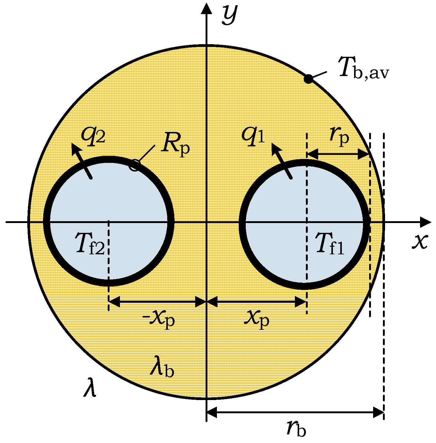
Figure 3 shows the case that is considered in this study. There are two symmetrically placed pipes in a grouted borehole. The center of the two pipes lie at (xp,0) and (−xp,0), respectively. The prescribed heat fluxes from the pipes are q1 and q2 (W/m). The corresponding fluid temperatures are Tf1 and Tf2. The main objective is to present a very precise method to calculate the relations between heat flows and fluid temperatures.
The primary input data are:
The thermal resistance may be represented by a dimensionless parameter β and the ratio between the two conductivities by the parameter σ. The circles of the pipes and the borehole should not intersect. This gives:
The number of equations and unknowns for multipole factors for two pipes are in general 2·2·J. But in the considered symmetrical case, the multipole factors Pn,j turn out to be real-valued numbers. The number of unknowns and equations are reduced to 2·J for the two sets of multipoles P1,j and P2,j.
4.1. Multipole Relations for Even and Odd Solutions
The multipoles for the two pipes depend on the prescribed heat fluxes. The temperature field is symmetric in x for equal heat fluxes:
The temperature field is odd in x for antisymmetric heat fluxes:
The average temperature at the borehole wall is chosen to be zero in both cases: Tb,av = 0.
There is a set of multipole factors for the even case and another one for the odd case. It is found for these two cases of high symmetry that the multipoles of pipe 2 are closely related to the multipoles of pipe 1 in the even and odd cases. The following relations are valid for the even case s = +1 and for the odd case s = −1:
The upper index + represents the even temperature solution and s = +1, while the upper index − represents the odd solution and s = −1. With these notational conventions, the formulas below for the even and odd cases can be presented in the same formulas, where s = ±1 becomes a parameter.
The temperature solutions for the even and odd cases determine the required fluid temperatures, which define an even and an odd thermal resistance and , respectively, in the following way:
These even and odd thermal resistances are obtained from the multipole solutions. They are the required fluid temperatures for unit heat flux. These thermal resistances depend on the choice of the number of multipoles J. It will be shown below that the accuracy increases rapidly with increasing J.
4.2. Formulas for Even and Odd Thermal Resistances
The temperature field of Equation (10) may be used without the right-hand sum of multipoles. In this case J = 0, and only the sum of line sources are used. The thermal resistances for the two symmetrically placed pipes then become:
The correction to the zero-order resistance for any positive J is given by a formula of the type:
The quantities and are obtained from the even and odd solutions for the considered multipole order J. In the formulas below the following auxiliary (dimensionless) parameters are used:
The B-values for any positive J are obtained from the formula:
The larger dot indicates a matrix/vector multiplication. The formula involves two vectors VJ and VbJ, and a matrix MJ for the even case s = +1 and the odd case s = −1:
Note that inverses of the M matrices appear in Equation (30). The components of the vectors VJ and VbJ are given by:
The M matrices are given by:
Here, the two matrices A+ and A−, which account for various interactions between line sources and multipoles in the boundary conditions at the two pipes, are fairly complicated:
It may be noted that the A matrices are symmetric.
The matrix formula, Equation (30), becomes a sum over all components of the inverse of the M matrix:
4.3. Explicit Multipole Formulas for First, Second and Third-Order
The zero-order resistances and are given by the explicit formulas of Equations (26) and (27), respectively. Explicit formulas may also be derived for J = 1 and J = 2.
The first-order corrections are given by Equation (35) for J = 1, in which case the inverse of the matrix is equal the inverse of the single matrix component:
The quantities in this formula are defined in Equations (32)–(34):
The final formula is then:
Here, the five dimensionless parameters are defined by Equations (20) and (29).
The second-order corrections are given by Equation (35) for J = 2:
The M matrices and their inverses are:
The first-order components in Equation (37) for J = 1 are still valid. The second-order components of the symmetric A matrices and V vectors are from Equations (32) and (34):
A more explicit formula can now be obtained from Equations (35), (39) and (40):
The third-order corrections for J = 3 involve the inversion of the 3 × 3 M matrices. A more explicit formula cannot be given. The third-order corrections are given by Equation (30) for J = 3:
Here, and are given by Equation (31) for J = 3. The M matrices have the form:
Here, is from Equation (34) for indices k or j equal to three. The third-order corrections of Equation (43) are given by Equation (45) for J = 3:
The formula contains all 9 components of the inverse matrix to .
4.4. Thermal Resistances R1b, R12, Rb and Ra
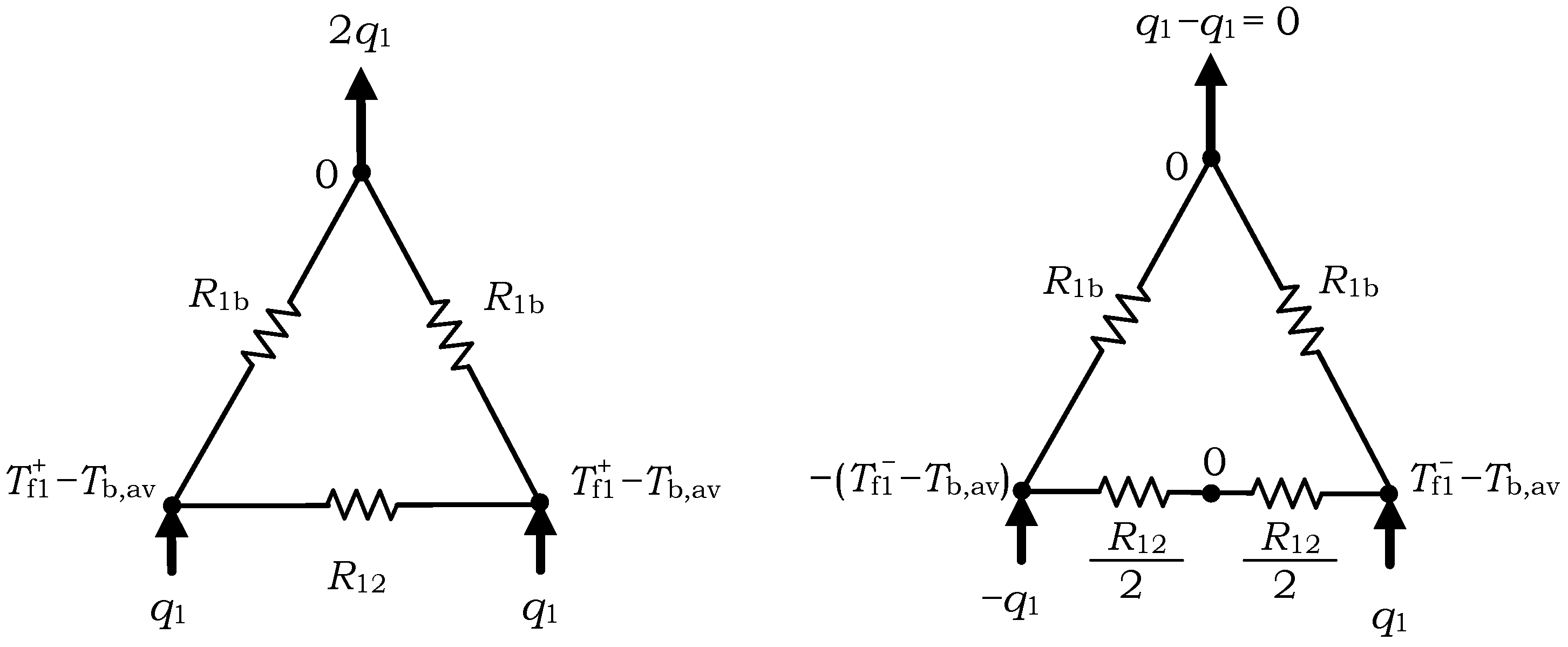
Final formulas for thermal resistances R1b, R12, Rb and Ra can now be obtained by again considering the Δ network of Figure 1. For the case of equal pipes in symmetric positions, the thermal resistances R1b is equal to R2b, and thus the heat fluxes of Equations (3) and (4) become:
Using Equations (24), (25) and (46), the thermal networks for even (q2 = q1) and odd (q2 = −q1) cases can be drawn as shown in Figure 4.
As seen from the even case of Figure 4, the borehole thermal resistance Rb between the fluid in pipes and the borehole wall consists of two parallel equal resistances, each of value R1b. On the other hand, from the odd case of Figure 4, it can be noticed that the total internal resistance Ra between the two pipes consists of a pair of equal series resistances, each of value 0.5 R12. Hence, Equations (5) and (6) can now be simplified to:
Final formulas for network resistances R1b and R12 are obtained in the form of even and odd thermal resistance and using Figure 4 and Equations (24) and (25).
Similarly, final formulas for thermal resistances Rb and Ra are obtained in the form of even and odd thermal resistance and using Equations (47) and (48).
For Equations (48) and (49), the values of thermal resistance and are obtained from Equations (28) and (38) for the first-order multipoles, from Equations (28) and (42) for the second-order multipoles, and from Equations (28) and (45) for the third-order multipoles.
5. Comparison with Existing Multipole Solutions
In this section, the new higher-order multipole formulas for borehole thermal resistance and total internal thermal resistance are compared with previously published results. The comparison is made using a reference dataset provided by [13], who compared and benchmarked the borehole thermal resistance estimations from ten different analytical methods against the tenth-order multipole method for 216 different cases. The authors showed that compared to other methods, the zeroth-order and first-order multipole formulas provide better accuracies over the entire range of studied parameters. In this paper, we will also benchmark the newly developed second-order and third-order multipole formulas against the tenth-order multipole method. The second-order and third-order multipole formulas will also be compared to each other and to the zeroth-order and first-order multipole formulas to demonstrate improvements in the accuracy of the calculated results.
Table 1 provides the detailed summary of the 216 comparison cases provided by the reference dataset used in this paper for the comparison of the second-order and third-order multipole formulas. The cases cover three different borehole diameters of 96 mm, 192 mm, and 288 mm. The U-tube outer pipe diameter value is held fixed at 32 mm for all cases. The total pipe resistance Rp also remains constant at 0.05 m-K/W. For each borehole diameter, three shank spacing configurations, i.e., close, moderate and wide, corresponding, respectively, to Paul’s [8] Configuration A, Configuration B and Configuration C, are considered. Four levels of ground thermal conductivity ranging from 1–4 W/m-K, and six levels of grout thermal conductivity ranging from 0.6–3.6 W/m-K are used. Given the existing and reasonably foreseeable values of design parameters, the 216 cases used for the comparison bracket almost all real-world single U-tube borehole heat exchangers.
Results of the second-order and third-order multipole formulas for calculating the grout thermal resistance and the total internal thermal resistance are summarized in Table 2 and Table 3, respectively. Each entry in these two tables represents the mean or maximum error in percentage for a sample containing two three values of grout thermal conductivity, three values of borehole diameter, and four values of ground thermal conductivity. The errors have been determined by comparing the results of multipole formulas to the tenth-order multipole method.
Table 2 shows that the grout thermal resistance (Rg) values obtained from the second-order and third-order multipole formulas are, respectively, within 0.5% and 0.2% of the tenth-order multipole method for all 216 cases. Also, the mean absolute percentage error of the results obtained from the second-order and third-order multipole formula are, respectively, smaller than 0.2% and 0.1%. In comparison, the mean and maximum absolute percentage errors for the zeroth-order multipole formula are as high as 9% and 30%, respectively. The first-order multipole formula has smaller errors than the zeroth-order formula. The mean and maximum absolute percentage errors for the first-order multipole formula are 0.7% and 2.2%, respectively.
Table 3 shows that the total internal thermal resistance (Ra) values calculated from the second order and third-order multipole formulas are, respectively, within 1% and 0.1% of the tenth-order multipole method for all 216 cases. The mean absolute percentage error of the results obtained from the second-order and third-order multipole formulas never exceed 0.4% and 0.1%, respectively. In comparison, the zeroth-order and the first-order multipole formulas give maximum absolute percentage errors of approximately 38% and 6%, respectively. The mean absolute percentage errors of the zeroth-order and the first-order multipole expressions are as high as 23% and 3%, respectively.
As shown and discussed above, compared to the zeroth-order and first-order multipole formulas, the accuracy of the newly developed second-order and third-order multipole formulas to calculate borehole thermal resistance and total internal thermal resistance is higher by several orders of magnitude. Even though the second-order and third-order multipole formulas presented in this paper are more complicated than other analytical expressions including the zeroth-order and first-order formulas, they are still simple enough to apply for computation purposes. The implementation of the second-order multipole formulas involves approximately ten lines of coding of rather compact and simple algebraic expressions. Whereas, the implementation of third-order multipole formulas requires programing of a more complex set of equations involving vector and matrix algebra.
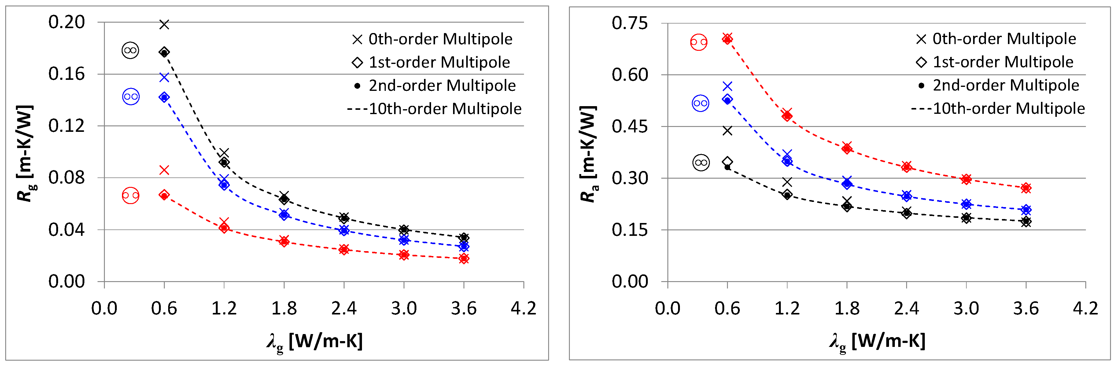
Although, both second-order and third-order multipole formulas offer a significant improvement over the original implementation of the multipole method, which required about 600 lines of FORTRAN coding, but the second-order multipole formulas are intrinsically more straightforward to implement, while providing almost similar levels of accuracy as third-order multipole formulas. Figure 5, Figure 6 and Figure 7 present a selection of representative comparison results of second-order multiple formulas against zeroth-order, first-order and tenth-order multipoles. The results shown in these figures are for a single ground thermal conductivity of 4.0 W/m-K. The left-side figures show the grout thermal resistance Rg values, and the right-side ones show the total internal thermal resistance Ra values, plotted against the grout thermal conductivity. Each figure presents three curves corresponding to close, moderate and wide shank spacings, shown in black, blue and red colors, respectively. The exact value of the shank spacing for each case is provided in Table 1. It must be pointed out that multipole formulas presented in the previous section, calculate the borehole thermal resistance and not the grout thermal resistance. However, in order to be consistent with the dataset provided by [13], the values of grout thermal resistance have been calculated and presented in Figure 5, Figure 6 and Figure 7. The grout thermal resistance values have been determined from Equation (2), by subtracting half of the fixed pipe resistance of 0.05 m-K/W from the corresponding borehole thermal resistance values obtained from the multipole formulas. Computing the grout thermal resistance directly by disregarding the pipe resistance gives erroneous results for all but zeroth-order multipole calculations.
Figure 5, Figure 6 and Figure 7 further demonstrate the ability of second-order multiple formulas to calculate the grout thermal resistance Rg and the total internal thermal resistance Ra. The thermal resistance values calculated from the second-order multiple formulas are always within 1% of the original tenth-order multipole method over the entire range of parameters. Hence, it can be concluded that due to their excellent accuracy and relative ease of implementation, the second-order multipole formulas are recommended for calculation of borehole thermal resistance and total internal thermal resistance for all cases where the two legs of the U-tube are placed symmetrically in the borehole.
6. Conclusions
This paper has presented new second-order and third-order multipole formulas for calculating borehole thermal resistance and total internal thermal resistance. The newly derived formulas can be used for all single U-tube applications where the two legs of the U-tube are symmetrically placed in the borehole. The presented formulas have been compared with the original multipole method, as well as the previously derived zeroth-order and first-order explicit multipole formulas. Both the second-order and third-order multipole formulas provide significant accuracy improvements over the zeroth-order and the first-order multipole formulations. The thermal resistances calculated from the second-order and third-order multipole formulas are always within 1% and 0.2% of the original tenth-order multipole method, respectively. Second-order multipole formulas are, however, more straightforward to use and are, thus, recommended for use in practice.
Acknowledgments
The support of both authors was provided by the Swedish Energy Agency (Energimyndigheten) through its national research program EFFSYS Expand. The funding source had no involvement in the study design; collection, analysis and interpretation of data; or in the decision to submit the article for publication.
Author Contributions
Both authors contributed equally in the design, concept, and preparation of the manuscript.
Conflicts of Interest
The authors declare no conflict of interest.
Nomenclature
| = | Multipole correction for multipole order J for even (+) and odd (−) cases, See Equation (30) | |
| bk | = | Dimensionless parameter, see Equation (29) |
| cf | = | Specific heat of the circulating fluid in the U-tube, J/kg-K |
| H | = | Depth of the borehole, m |
| J | = | Number of multipoles, j = 0, 1, 2, …, J |
| N | = | Number of pipes in the borehole; N = 2 for single U-tube |
| Pn,j | = | Multipole factor of order j for pipe n |
| = | Multipole factor of order j for pipe n for even (+) and odd (−) cases | |
| p0 | = | Dimensionless parameter, see Equation (29) |
| p1 | = | Dimensionless parameter, see Equation (29) |
| p2 | = | Dimensionless parameter, see Equation (29) |
| qb | = | Heat rejection rate per unit length of borehole, W/m |
| qn | = | Heat rejection rate per unit length of pipe n, W/m |
| Ra | = | Total internal borehole thermal resistance, m-K/W |
| Rb | = | Local borehole thermal resistance between fluid in the U-tube to borehole wall, m-K/W |
| = | Effective borehole thermal resistance, m-K/W | |
| Rg | = | Grout thermal resistance, m-K/W |
| = | Thermal resistance for even (+) and odd (−) cases for J multipoles, m-K/W | |
| Rnb | = | Thermal resistance between U-tube leg n and borehole wall, m-K/W |
| Rp | = | Total fluid-to-pipe resistance for a single pipe i.e., one leg of the U-tube, m-K/W |
| R12 | = | Thermal resistance between U-tube legs 1 and 2, m-K/W |
| rb | = | Radius of the borehole, m |
| rp | = | Outer radius of the pipe making up the U-tube, m |
| Tb | = | Borehole wall temperature, °C |
| Tb,av | = | Average temperature at the borehole wall, °C |
| Tf | = | Mean fluid temperature inside the U-tube, °C |
| Tf,loc | = | Local mean fluid temperature, °C |
| Tfn | = | Fluid temperature in U-tube leg n, °C |
| = | Fluid temperature in U-tube leg n for even and odd cases, °C | |
| Vf | = | Volume flow rate of the circulating fluid in the U-tube, m3/s |
| xp | = | Half shank spacing; half of center-to-center distance between U-tube legs, m, See Figure 3 |
| β | = | Dimensionless thermal resistance of one U-tube leg, see Equation (20) |
| λ | = | Thermal conductivity of the ground, W/m-K |
| λb | = | Thermal conductivity of the borehole/grout, W/m-K |
| = | Density of the circulating fluid in the U-tube, kg/m3 | |
| σ | = | Thermal conductivity ratio, dimensionless, see Equation (20) |
References
- Lund, J.W.; Boyd, T.L. Direct utilization of geothermal energy 2015 worldwide review. Geothermics 2016, 60, 66–93. [Google Scholar] [CrossRef]
- Vieira, A.; Alberdi-Pagola, M.; Christodoulides, P.; Javed, S.; Loveridge, F.; Nguyen, F.; Cecinato, F.; Maranha, J.; Florides, G.; Prodan, I.; et al. Characterisation of ground thermal and thermo-mechanical behaviour for shallow geothermal energy applications. Energies 2017, 10, 2044. [Google Scholar] [CrossRef]
- Javed, S.; Spitler, J.D. Calculation of borehole thermal resistance. In Advances in Ground-Source Heat Pump Systems, 1st ed.; Rees, S.J., Ed.; Woodhead Publishing: Cambridge, UK, 2016; pp. 63–95. ISBN 978-0-08-100311-4. [Google Scholar]
- Spitler, J.D.; Gehlin, S.E. Thermal response testing for ground source heat pump systems—An historical review. Renew. Sustain. Energy Rev. 2015, 50, 1125–1137. [Google Scholar] [CrossRef]
- Kavanaugh, S.P. Simulation and Experimental Verification of Vertical Ground-Coupled Heat Pump Systems. Ph.D. Thesis, Oklahoma State University, Stillwater, OK, USA, May 1985. [Google Scholar]
- Gu, Y.; O’Neal, D.L. Development of an equivalent diameter expression for vertical U-tubes used in ground-coupled heat pumps. ASHRAE Trans. 1998, 104, 347–355. [Google Scholar]
- Shonder, J.A.; Beck, J.V. Field test of a new method for determining soil formation thermal conductivity and borehole resistance. ASHRAE Trans. 2000, 106, 843–850. [Google Scholar]
- Paul, N.D. The Effect of Grout Thermal Conductivity on Vertical Geothermal Heat Exchanger Design and Performance. Master’s Thesis, South Dakota University, Brookings, SD, USA, July 1996. [Google Scholar]
- Sharqawy, M.H.; Mokheimer, E.M.; Badr, H.M. Effective pipe-to-borehole thermal resistance for vertical ground heat exchangers. Geothermics 2009, 38, 271–277. [Google Scholar] [CrossRef]
- Bauer, D.; Heidemann, W.; Müller-Steinhagen, H.; Diersch, H.J. Thermal resistance and capacity models for borehole heat exchangers. Int. J. Energy Res. 2011, 35, 312–320. [Google Scholar] [CrossRef]
- Liao, Q.; Zhou, C.; Cui, W.; Jen, T.C. New correlations for thermal resistances of vertical single U-Tube ground heat exchanger. J. Therm. Sci. Eng. Appl. 2012, 4, 031010. [Google Scholar] [CrossRef]
- Lamarche, L.; Kajl, S.; Beauchamp, B. A review of methods to evaluate borehole thermal resistances in geothermal heat-pump systems. Geothermics 2010, 39, 187–200. [Google Scholar] [CrossRef]
- Javed, S.; Spitler, J.D. Accuracy of borehole thermal resistance calculation methods for grouted single U-tube ground heat exchangers. Appl. Energy 2017, 187, 790–806. [Google Scholar] [CrossRef]
- Bennet, J.; Claesson, J.; Hellström, G. Multipole Method to Compute the Conductive Heat Flows to and between Pipes in a Composite Cylinder. Notes on Heat Transfer 3; University of Lund: Lund, Sweden, 1987. [Google Scholar]
- Claesson, J.; Bennet, J. Multipole Method to Compute the Conductive Heat Flows to and between Pipes in a Cylinder. Notes on Heat Transfer 2; University of Lund: Lund, Sweden, 1987. [Google Scholar]
- Claesson, J.; Hellström, G. Multipole method to calculate borehole thermal resistances in a borehole heat exchanger. HVAC R Res. 2011, 17, 895–911. [Google Scholar]
- Young, T.R. Development, Verification, and Design Analysis of the Borehole Fluid Thermal Mass Model for Approximating Short Term Borehole Thermal Response. Ph.D. Thesis, Oklahoma State University, Stillwater, OK, USA, December 2004. [Google Scholar]
- He, M. Numerical Modelling of Geothermal Borehole Heat Exchanger Systems. Ph.D. Thesis, De Montfort University, Leicester, UK, February 2012. [Google Scholar]
- Al-Chalabi, R. Thermal Resistance of U-Tube Borehole Heat Exchanger System: Numerical Study. Master’s Thesis, University of Manchester, Manchester, UK, September 2013. [Google Scholar]
- Earth Energy Designer (EED), v3.2; BLOCON: Lund, Sweden, 2015.
- Spitler, J.D. GLHEPRO—A Design Tool for Commercial Building Ground Loop Heat Exchangers. In Proceedings of the Fourth International Heat Pumps in Cold Climates Conference, Aylmer, QC, Canada, 17–18 August 2000. [Google Scholar]
- Claesson, J. Multipole Method to Calculate Borehole Thermal Resistances; Mathematical Report; Chalmers University of Technology: Gothenburg, Sweden, 2012. [Google Scholar]
- Hellström, G. Ground Heat Storage—Thermal Analyses of Duct Storage Systems—Theory. Ph.D. Thesis, University of Lund, Lund, Sweden, April 1991. [Google Scholar]
- Spitler, J.D.; Javed, S.; Ramstad, R.K. Natural convection in groundwater-filled boreholes used as ground heat exchangers. Appl. Energy 2016, 164, 352–365. [Google Scholar] [CrossRef]
- Zeng, H.; Diao, N.; Fang, Z. Heat transfer analysis of boreholes in vertical ground heat exchangers. Int. J. Heat Mass Transf. 2003, 46, 4467–4481. [Google Scholar] [CrossRef]
- Ma, W.; Li, M.; Li, P.; Lai, A.C. New quasi-3D model for heat transfer in U-shaped GHEs (ground heat exchangers): Effective overall thermal resistance. Energy 2015, 90, 578–587. [Google Scholar] [CrossRef]
Figure 1.
Δ resistance network for a single U-tube in a borehole.

Figure 2.
Steady-state heat conduction in a composite circular region with heat flows between N number of pipes and the adjacent ground region.
Figure 2.
Steady-state heat conduction in a composite circular region with heat flows between N number of pipes and the adjacent ground region.

Figure 3.
Two symmetrically placed pipes in a grouted borehole.

Figure 4.
Thermal resistance networks for equal pipes in symmetric positions for even (left) and odd (right) cases.
Figure 4.
Thermal resistance networks for equal pipes in symmetric positions for even (left) and odd (right) cases.

Figure 5.
Grout thermal resistance (Rg) and total internal resistance (Ra) for close (2xp = 32 mm), moderate (2xp = 43 mm) and wide (2xp = 64 mm) configurations with 2rb = 96 mm and λ = 4 W/m-K.
Figure 5.
Grout thermal resistance (Rg) and total internal resistance (Ra) for close (2xp = 32 mm), moderate (2xp = 43 mm) and wide (2xp = 64 mm) configurations with 2rb = 96 mm and λ = 4 W/m-K.

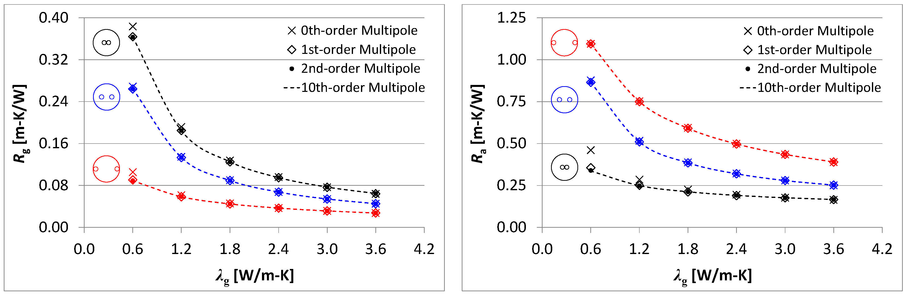
Figure 6.
Grout thermal resistance (Rg) and total internal resistance (Ra) for close (2xp = 32 mm), moderate (2xp = 75 mm) and wide (2xp = 160 mm) configurations with 2rb = 192 mm and λ = 4 W/m-K.
Figure 6.
Grout thermal resistance (Rg) and total internal resistance (Ra) for close (2xp = 32 mm), moderate (2xp = 75 mm) and wide (2xp = 160 mm) configurations with 2rb = 192 mm and λ = 4 W/m-K.

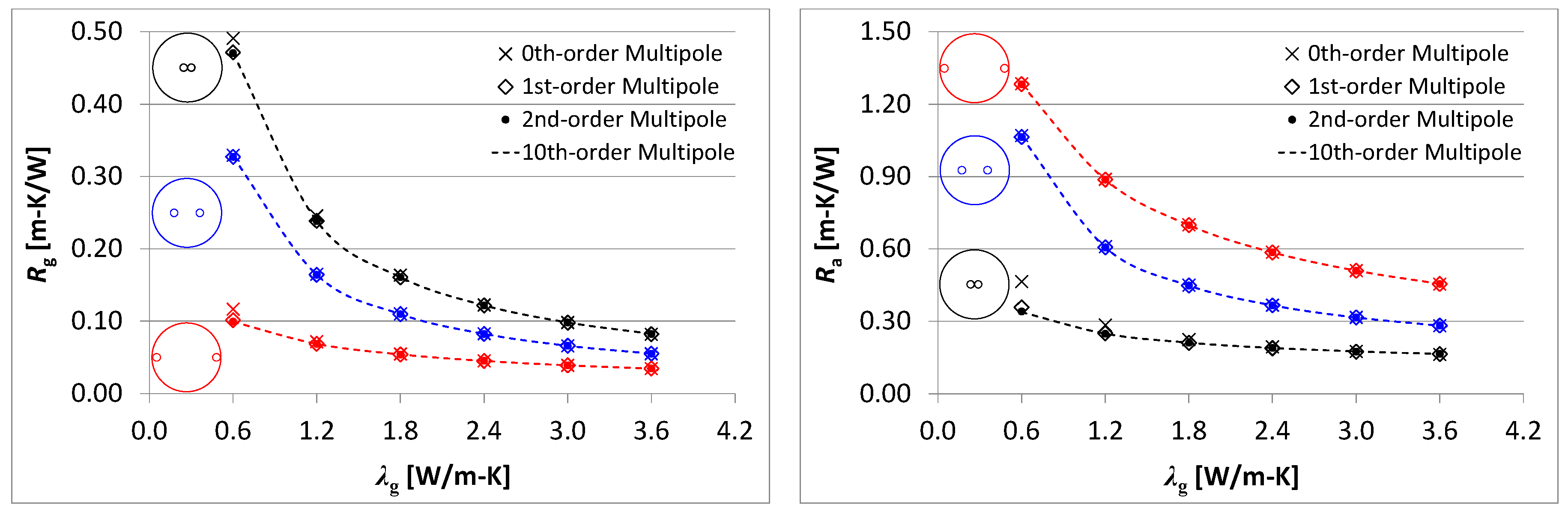
Figure 7.
Grout thermal resistance (Rg) and total internal resistance (Ra) for close (2xp = 32 mm), moderate (2xp = 107 mm) and wide (2xp = 256 mm) configurations with 2rb = 288 mm and λ = 4 W/m-K.
Figure 7.
Grout thermal resistance (Rg) and total internal resistance (Ra) for close (2xp = 32 mm), moderate (2xp = 107 mm) and wide (2xp = 256 mm) configurations with 2rb = 288 mm and λ = 4 W/m-K.


Table 1.
Summary of comparison cases provided by [13].
Table 1.
Summary of comparison cases provided by [13].
| Parameters | Levels | No. of Levels |
|---|---|---|
| Ratio of borehole diameter to outer pipe diameter 1, 2rb/2rp | 3, 6, 9 | 3 |
| Shank spacing configuration, 2xp (mm) | Close, Moderate, Wide 2 For rb/rp = 3, 2xp = 32, 43, 64 For rb/rp = 6, 2xp = 32, 75, 160 For rb/rp = 9, 2xp = 32, 107, 256 | 3 |
| Ground thermal conductivity, λ (W/m-K) | 1, 2, 3, 4 | 4 |
1 Pipe outer diameter (2rp) is fixed at 32 mm, borehole diameters (2rb) are 96 mm, 192 mm, and 288 mm. 2 Corresponding to Paul’s [8] A–C configurations.
Table 2.
Mean and maximum absolute percentage errors in calculation of the grout thermal resistance (Rg) for the 216 cases provided by [13].
Table 2.
Mean and maximum absolute percentage errors in calculation of the grout thermal resistance (Rg) for the 216 cases provided by [13].
| Method | Shank Spacing Configuration | Ground Conductivity | |||||
|---|---|---|---|---|---|---|---|
| Low (0.6–1.2 W/m-K) | Moderate (1.2–2.4 W/m-K) | High (2.4–3.6 W/m-K) | |||||
| Mean | Max | Mean | Max | Mean | Max | ||
| Zeroth-order multipole | Close | 6.1 | 12.4 | 2.9 | 8.0 | 1.0 | 2.5 |
| Moderate | 3.3 | 10.8 | 1.5 | 6.5 | 0.4 | 1.6 | |
| Wide | 8.9 | 30.4 | 1.9 | 11.2 | 0.3 | 1.8 | |
| First-order multipole | Close | 0.2 | 0.4 | 0.2 | 0.6 | 0.7 | 1.5 |
| Moderate | 0.0 | 0.2 | 0.0 | 0.2 | 0.1 | 0.5 | |
| Wide | 0.5 | 2.2 | 0.0 | 0.2 | 0.1 | 0.6 | |
| Second-order multipole | Close | 0.0 | 0.0 | 0.1 | 0.2 | 0.2 | 0.5 |
| Moderate | 0.0 | 0.0 | 0.0 | 0.1 | 0.0 | 0.1 | |
| Wide | 0.1 | 0.3 | 0.0 | 0.0 | 0.0 | 0.1 | |
| Third-order multipole | Close | 0.0 | 0.0 | 0.0 | 0.1 | 0.1 | 0.2 |
| Moderate | 0.0 | 0.0 | 0.0 | 0.0 | 0.0 | 0.0 | |
| Wide | 0.0 | 0.0 | 0.0 | 0.0 | 0.0 | 0.0 | |
Table 3.
Mean and maximum absolute percentage errors in calculation of the total internal thermal resistance (Ra) for the 216 cases provided by [13].
Table 3.
Mean and maximum absolute percentage errors in calculation of the total internal thermal resistance (Ra) for the 216 cases provided by [13].
| Method | Shank Spacing Configuration | Ground Conductivity | |||||
|---|---|---|---|---|---|---|---|
| Low (0.6–1.2 W/m-K) | Moderate (1.2–2.4 W/m-K) | High (2.4–3.6 W/m-K) | |||||
| Mean | Max | Mean | Max | Mean | Max | ||
| Zeroth-order multipole | Close | 23.3 | 37.6 | 6.9 | 15.0 | 1.2 | 2.7 |
| Moderate | 1.8 | 7.8 | 1.1 | 6.0 | 0.3 | 1.8 | |
| Wide | 1.9 | 8.5 | 0.4 | 2.3 | 0.2 | 1.3 | |
| First-order multipole | Close | 3.2 | 5.9 | 0.6 | 0.7 | 0.7 | 0.7 |
| Moderate | 0.2 | 0.8 | 0.0 | 0.2 | 0.1 | 0.2 | |
| Wide | 0.3 | 1.2 | 0.0 | 0.1 | 0.0 | 0.1 | |
| Second-order multipole | Close | 0.4 | 1.0 | 0.2 | 0.2 | 0.1 | 0.2 |
| Moderate | 0.0 | 0.0 | 0.0 | 0.0 | 0.0 | 0.0 | |
| Wide | 0.0 | 0.2 | 0.0 | 0.0 | 0.0 | 0.0 | |
| Third-order multipole | Close | 0.0 | 0.1 | 0.1 | 0.1 | 0.0 | 0.0 |
| Moderate | 0.0 | 0.0 | 0.0 | 0.0 | 0.0 | 0.0 | |
| Wide | 0.0 | 0.0 | 0.0 | 0.0 | 0.0 | 0.0 | |
© 2018 by the authors. Licensee MDPI, Basel, Switzerland. This article is an open access article distributed under the terms and conditions of the Creative Commons Attribution (CC BY) license (http://creativecommons.org/licenses/by/4.0/).
Share and Cite
MDPI and ACS Style
Claesson, J.; Javed, S. Explicit Multipole Formulas for Calculating Thermal Resistance of Single U-Tube Ground Heat Exchangers. Energies 2018, 11, 214. https://doi.org/10.3390/en11010214
AMA Style
Claesson J, Javed S. Explicit Multipole Formulas for Calculating Thermal Resistance of Single U-Tube Ground Heat Exchangers. Energies. 2018; 11(1):214. https://doi.org/10.3390/en11010214
Chicago/Turabian StyleClaesson, Johan, and Saqib Javed. 2018. "Explicit Multipole Formulas for Calculating Thermal Resistance of Single U-Tube Ground Heat Exchangers" Energies 11, no. 1: 214. https://doi.org/10.3390/en11010214
Note that from the first issue of 2016, this journal uses article numbers instead of page numbers. See further details here.