Net Load Carrying Capability of Generating Units in Power Systems


Department of Energy System Engineering, Chung-Ang University, 84 Heukseok-ro, Dongjak-gu, Seoul 06974, Korea
*
Author to whom correspondence should be addressed.
Energies 2017, 10(8), 1221; https://doi.org/10.3390/en10081221
Submission received: 12 July 2017
/
Revised: 4 August 2017
/
Accepted: 11 August 2017
/
Published: 17 August 2017
(This article belongs to the Special Issue Risk-Based Methods Applied to Power and Energy Systems)
Abstract
:This paper proposes an index called net load carrying capability (NLCC) to evaluate the contribution of a generating unit to the flexibility of a power system. NLCC is defined as the amount by which the load can be increased when a generating unit is added to the system, while still maintaining the flexibility of the system. This index is based on the flexibility index termed ramping capability shortage expectation (RSE), which has been used to quantify the risk associated with system flexibility. This paper argues that NLCC is more effective than effective load carrying capability (ELCC) in quantifying the contribution of the generating unit to flexibility. This is explained using an illustrative example. A case study has been performed with a modified IEEE-RTS-96 to confirm the applicability of the NLCC index. The simulation results demonstrate the effect of operating conditions such as operating point and ramp rate on NLCC, and show which kind of unit is more helpful in terms of flexibility.
1. Introduction
The high penetration of renewable energy resources (RES) has made it more difficult to secure flexibility in power systems, which is defined as the ability to respond to changes in net load, i.e., load minus output of non-dispatchable RES [1,2,3,4]. System planners and operators have tried to secure an adequate level of reserve capacity in view of reliability. However, this approach does not guarantee flexibility, because the problem can be caused by a shortage in ramping capability (i.e., the ability to change the output of a generating unit in a given period), despite there being sufficient reserve capacity [5,6]. With respect to this problem, some researchers have noted the role of the generating unit in enabling the system to secure flexibility by providing the required ramping capability, which must be the most effective measure to cope with a net load variation [7,8,9,10]. The greater the ramping capability, the stronger the ability of the system to react to unexpected changes in net load; that is, larger and faster units are helpful for coping with the flexibility issue.
This issue is directly related to both generation scheduling and generation expansion planning (GEP) [11,12,13,14]. In particular, special care is required when establishing GEP to manage the operational risks related to flexibility, as the integration of RES increases [15,16,17,18]. In this situation, system planners and operators should consider which unit is more advantageous in terms of flexibility; that is, the extent to which a new unit contributes to flexibility should be evaluated. To the best of our knowledge, [19] this is the first study on the contribution of a generating unit to the flexibility of a power system. The authors proposed the effective ramping capability (ERC), which is based on an index called the inadequate ramping resource probability (IRRP), which is devised to capture the risk of insufficient ramping capability. However, the causal relationship between risk and uncertainty is not reflected in the IRRP, and this is essential because uncertainty is a source of risk, and cannot be separated from the countermeasures against risk [20]. IRRP underlies ERC; thus, ERC has a limitation for evaluating the contribution of a generating unit to flexibility.
This paper presents an index termed net load carrying capability (NLCC) to quantify the contribution of a generating unit to the flexibility of the power system. NLCC is applied to a generating unit in a similar way to the effective load carrying capability (ELCC), and is defined as the amount by which the net load can be increased, while maintaining flexibility, when the unit is added to the system. By using a risk index termed the ramping capability shortage expectation (RSE), the NLCC index is capable of capturing the risk of power mismatch events due to a shortage of ramping capability as well as lack of reserve capacity. An illustrative example shows that NLCC is more effective than ELCC to quantify the contribution of a generating unit to the flexibility of the system. A case study for a modified IEEE-RTS-96 has been performed to investigate the applicability of NLCC and to show the effect of operating conditions on the NLCC.
The remainder of this study is organized as follows. Section 2 explains the concept and calculation method of the NLCC index. In Section 3, an illustrative example is described to compare NLCC with ELCC. In Section 4, a case study for a modified IEEE-RTS-96 is conducted to show the applicability of NLCC and to confirm the effect of the operating conditions on NLCC. The conclusion and future works are presented in Section 5.
2. Net Load Carrying Capability
ELCC has been used to evaluate the contribution of a generating unit to the reliability of a power system [21,22,23,24,25,26]. It is defined as the amount of increase in load that maintains reliability when the considered unit is added to the system, and is measured using a reliability index, such as loss of load probability (LOLP) or loss of load expectation (LOLE) [27,28]. These reliability indices have limitations in capturing short-term operating conditions, which are necessary for capturing the system flexibility. The ELCC index has similar limitations in catching the system flexibility. A previous study [29] attempted to evaluate ELCC based on the security constrained unit commitment (SCUC) model, where short-term operating conditions are considered along with stochastic scenarios for uncertainty. However, the reliability index is combined with the objective function, and therefore produces impure results. This kind of problem is unavoidable in an approach that utilizes the reliability index [30]. In this paper, the flexibility index RSE, which is able to reflect the operating conditions, is used instead of the reliability index [20].
2.1. Ramping Capability Shortage Probability (RSP) and Ramping Capability Shortage Expectation (RSE)
The RSPt is defined as the sum of the probabilities that net load variation during an interval between t − Δt and t could not be covered by the ramping capability of the system, as follows:
and the RSE is calculated by adding all RSPt as follows:
here, the terms on the left-hand side of the inequality sign imply the net load at time t, and the terms to the right mean the maximum output that all generating units can reach within Δt from t − Δt. NLFEt and Oi,t−Δt represent the uncertainty parameters in the net load and generation, respectively. Probc calculates the probability of whether all of the generating units are capable of compensating for the change in net load. Oi,t−Δt reflects the uncertainty scenario for the unit failure. The failure probability of the generating unit according to each scenario is calculated using the Markov chain-based capacity state model [31]. For detailed information on the RSE, please refer to [20].
2.2. Net Load Carrying Capability (NLCC)
The NLCC of a generating unit is defined as the amount of net load increase required to maintain flexibility (measured as RSE) when a unit is added to the system. The calculation procedure of NLCC is as follows:
Step 1: Calculate the RSE for the system before the unit is added.
Step 2: Calculate the RSE with changes in net load within a certain range (of course, the range is adjustable according to system).
Step 3: Add a new unit into the system. Vary the net load within a certain range, keeping all other data fixed, and calculate the RSE for the new system.
Step 4: The NLCC is the difference between the net load level with the RSE criterion in Step 2 and that in Step 3.
For reference, any flexible resource, such as a demand side resource, can be evaluated according to the steps above by modeling it as generating unit.
3. Comparison of NLCC with ELCC
The definition of NLCC is different from that of ELCC in the following terms: net load (instead of load), flexibility (instead of reliability), and RSE (instead of LOLE). Among these terms, RSE is an important factor, which makes a great difference between NLCC and ELCC. The differences between RSE and LOLE and between NLCC and ELCC are explained in detail using the following example.
3.1. Description of Illustrative Example
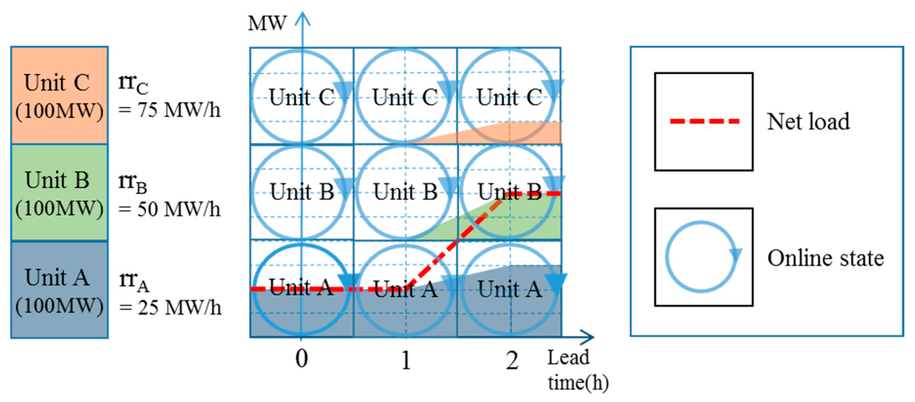
In the peak day of the targeted year, the forecast net loads at 0 h, 1 h, and 2 h are 50 MW, 50 MW, and 150 MW, respectively. The net load forecast error is neglected for simplicity. The number of the preexisting units is three; the capacity of each unit is 100 MW; their ramp-up rates are 25 MW/h (Unit A), 50 MW/h (Unit B), and 75 MW/h (Unit C), respectively. The generation schedule is determined following the merit-order principle, and the result is presented in Figure 1. All units are in online states; thus, a two-state capacity state model is used to calculate their failure probabilities. The failure rates of all of the units are 1/2940 (occurrences/h), and the repair rates are 1/60 (occurrences/h). A new unit, Unit D, which has the capacity of 100 MW and ramp rate of 40 MW/h, is considered to be added; it also has the lowest priority in the merit order. In this example, the value of Δt is assumed to be 1 h, and NLFEt is not considered for simplicity. The values of RSE and LOLE for the system without Unit D are selected as the RSE and LOLE criterion, respectively.
3.2. Comparison of RSE and LOLE
The calculation of LOLE determines whether the net load level is larger than the sum of the installed capacity every time. It is not concerned with whether the generating unit can be committed into operation or can raise output to follow changes in the net load; that is, the operating conditions of the generating units are neglected. In this example, the outage events occur only when the numbers of failed units are more than 3, 3, and 2 at 0, 1, and 2 h, respectively. This means that the outage events are irrelevant with the operating conditions of the units according to the generation schedule. For the details of the LOLE calculation, refer to Appendix A.
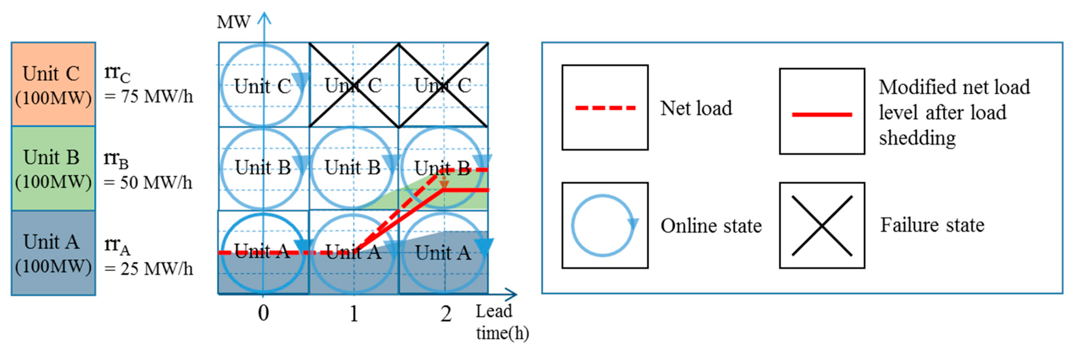
Meanwhile, it should be noted that the outage events could occur due to the shortage of ramping capability, even if the total capacity of the online units is larger than the net load level. Figure 2 shows how the failure of Unit B at 1 h can result in load shedding. The load shedding lasts for an hour, though Units A and B raise output to satisfy the net load increase after Unit C failed. Unlike LOLE, cases as this one are considered in the calculation of RSE. This is a major difference between RSE and LOLE.
3.3. Calculation Procedure of NLCC
Step 1: The RSE is applied to the worst-case scenario, where failure events occur just before the targeted time. For example, when estimating RSP2 (for reference, the RSE is the sum of every RSPt.), the failure scenario at 1 h is considered. Likewise, the failure scenario at 0 h is selected for RSP1. When considering the worst-case scenario, RSP1 and RSP2 are calculated, but RSP0 is not because there is no information before 0 h. Based on the Markov chain-based capacity state model, the failure probabilities for all units are calculated as at 0 h, and at 1 h. Table 1 shows whether a load-shedding event occurs, depending on failure cases and the consequential RSPt. For example, load shedding does not occur at 1 h as a consequence of the failure of Unit A at 0 h, and the corresponding failure probability at 0 h is calculated as . The RSPt is the sum of probabilities of the failure cases causing load-shedding events. For example, the RSP2 can be computed using Equation (1) as follows:
The failure cases that the FNL2 is larger than the value on right-hand side include ‘A’, ‘B’, ‘A&B’, ‘A&C’, ‘B&C’, and ‘A&B&C’ (corresponding to the failure cases at 1 h causing the load shedding event at 2 h). Adding all RSPt, RSE is determined as h/period, and this value is selected as the RSE criterion.
Step 2: The load level is varied within a range from 0% to 50%, with a step size of 5%. For reference, when the load variance is 5%, the forecast net loads at 0 h, 1 h, and 2 h are 52.5 MW, 52.5 MW, and 157.5 MW, respectively. By repeating Step 1 for each load variance, Table 2 can be obtained.
Step 3: Unit D is added to the system. As shown in Table 3, the failure cases and consequential load sheddings according to the addition of Unit D are newly calculated for each load variance. For the same load variance, the RSE in Table 3 is smaller than that in Table 2. It is because the addition of the unit improves the ramping capability of the system.
Step 4: The RSE value is larger than the RSE criterion (i.e., h/period) when the load variance is 20%. In order to find a point matching with the RSE criterion, the load variances are increased by 1% in each step from 15% to 20%, and the corresponding RSE are derived. The RSE begins to exceed the RSE criterion when the load variance is 16%; thus, in this example, the NLCC is equal to the peak load (i.e., 150 MW) multiplied by 15%, that is, 22.5 MW. This value is 27 MW smaller than the ELCC of 49.5 MW (refers to Appendix A.2). This difference is due to a shortage of ramp capability, which is caused by the operating conditions of each generating unit, such as operating point, maximum generation level, and ramp rate. Unlike ELCC, those conditions can be taken into account by the NLCC.
4. Case Study
4.1. Basic Information
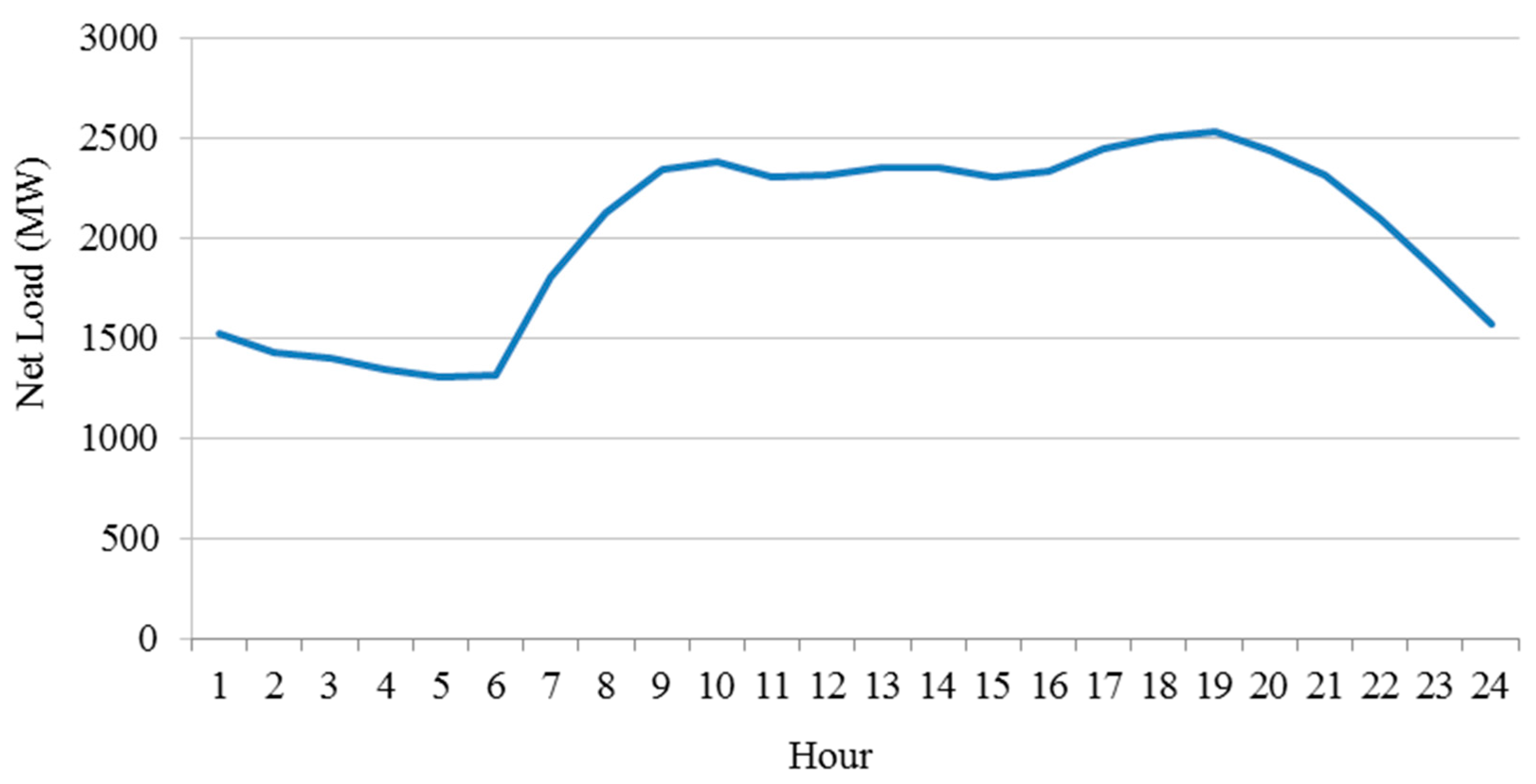
The main objective of our study is to examine the applicability of the NLCC index. The simulation is conducted with a modified IEEE-RTS-96 without the hydroelectric generating unit [31]. The number and installed capacity of the pre-existing generating units are 26 and 3105 MW, respectively. The applied failure and repair rates of all the units are included in Table A5 in Appendix B. A wind power plant with an installed capacity of 1250 MW is included in the system; its capacity value (as measured by ELCC) is calculated as 79.88 MW [32]. The forecasted net load profile is shown in Figure 3, where the peak load of 2531 MW occurs at hour 19. The ratio of installed capacity to peak load is 22.7%. The generation schedule considered is the hourly unit commitment, which is solved with dynamic programming [33]. It is assumed that all of the units are ready to be committed into operation at any time. The NLFE is assumed to follow a normal distribution, where the standard deviation is 5% of the forecasted net load. The RSE of h/day is used as the RSE criterion.
4.2. Scenario 1: Addition of a 400-MW Unit
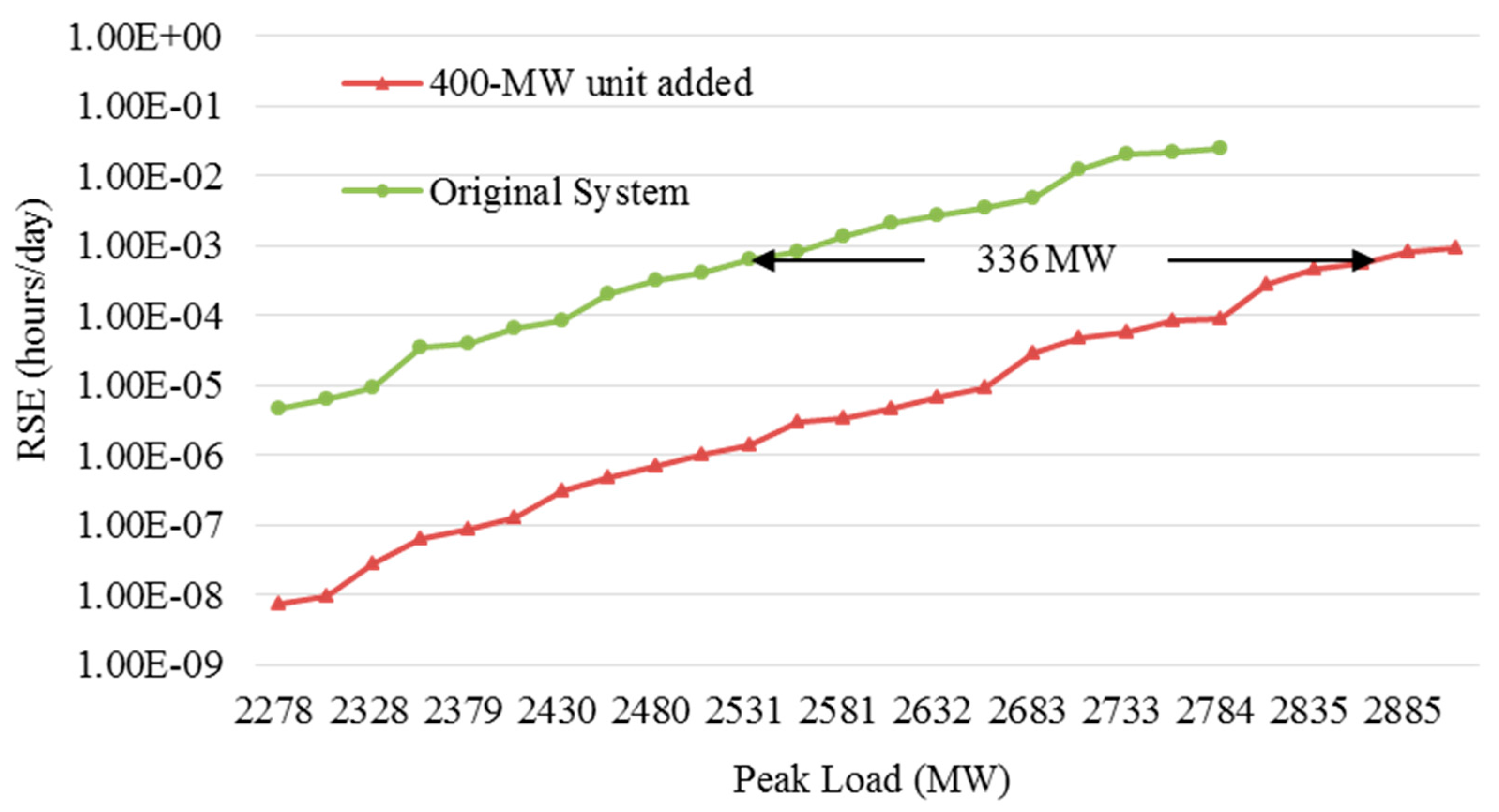
A 400-MW unit with a ramp rate of 1200 MW/h is added to the system. Its failure and repair rates are 1/1100 and 1/150 occurrences/h, respectively. The RSE values before and after adding the new unit are calculated according to the load variances, as shown in Figure 4. The NLCC at the designed level of flexibility (i.e., h/day) is 336 MW, which is about 84% of its installed capacity. This unit can technically provide its entire ramping capability every time; however, its ramping capability is somewhat restricted in some periods. The reason is that this unit maintains high levels of generation output over most of the whole period because of its high priority in merit order. Meanwhile, the effect of ramp rate on the NLCC is also tested. The ramp rate is adjusted to 200 MW/h (one sixth of the original value) and the simulation is carried out, with no change compared to the original result.
4.3. Scenario 2: Addition of a 100-MW Unit
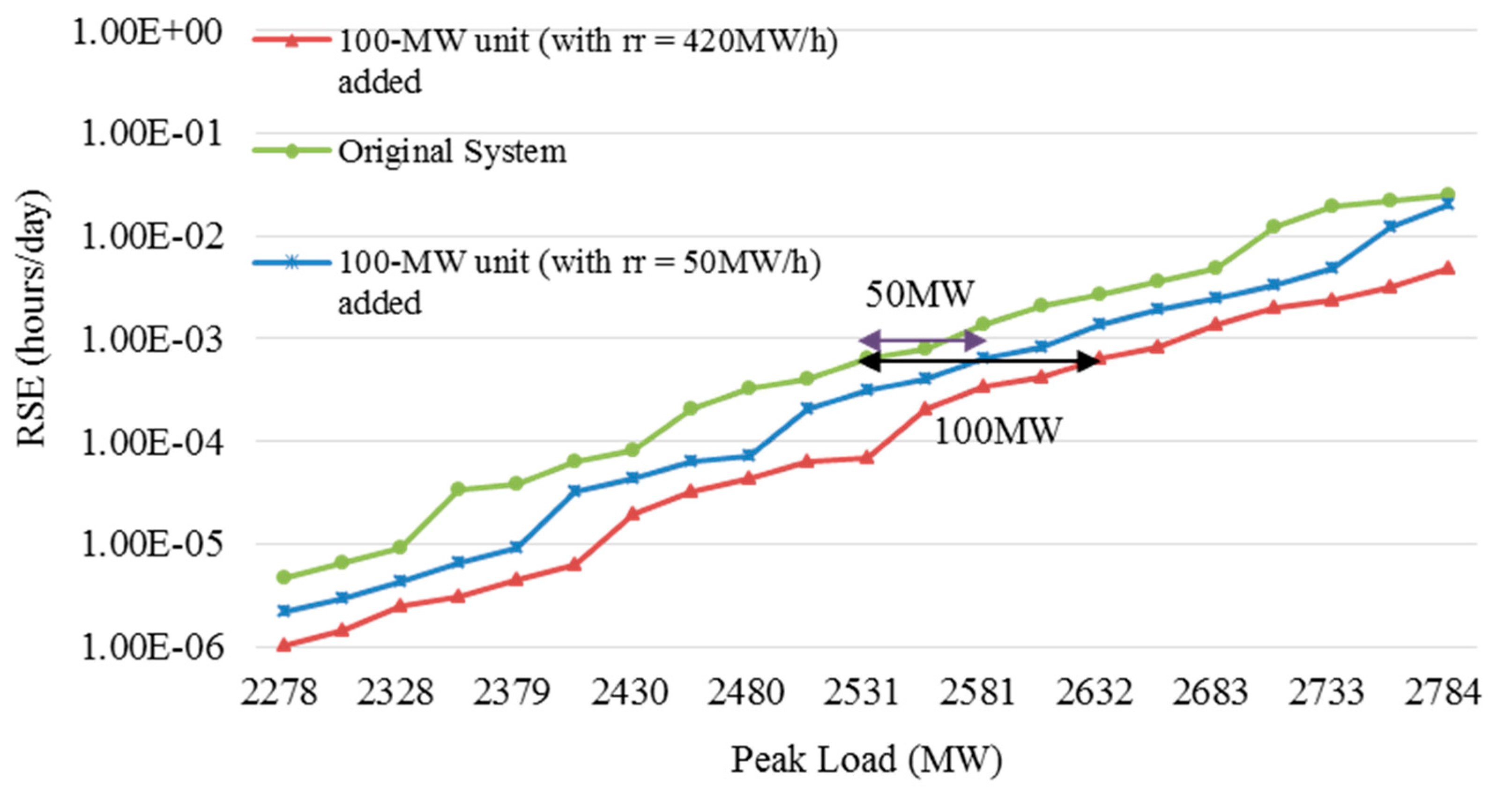
A 100-MW unit with a ramp rate of 420 MW/h is added to the system. Its failure and repair rates are 1/1200 and 1/50 occurrences/h, respectively. The RSE values before and after adding this unit are shown in Figure 5. The NLCC at the designed level of flexibility is 100 MW, which means that this unit can provide its entire ramping capability during the whole period. Unlike Scenario 1, this unit maintains low levels of generation output over most of the period, because it has a lower priority in the merit order; thus, the unit provides greater reserve capacity. In this situation, the impact of the change in ramp rate (i.e., the consequential change in ramping capability) on the NLCC is also investigated. The ramp rate is adjusted to 50 MW/h; accordingly, the NLCC of 50 MW is derived.
It should be noted that two factors—priority in merit order and ramp rate—affect the NLCC by changing the operating conditions. The higher the priority in the merit order, the smaller the extra reserve capacity of the unit, and therefore the NLCC is decreased. On the other hand, when the priority in the merit order is low, the ramp rate is larger, and the NLCC is higher. However, if the ramp rate of a generating unit is equal to or larger than the rating divided by an hour, then the NLCC does not vary with the ramp rate. This occurs because the unit can raise the output to its maximum value within an hour, whatever the ramp rate.
4.4. Scenario 3: Generation Expansion Planning (GEP)
Table 4 presents the load growth scenario with an annual increment of 7%. Four types of generating unit, as shown in Table 5, are considered candidates for this GEP.
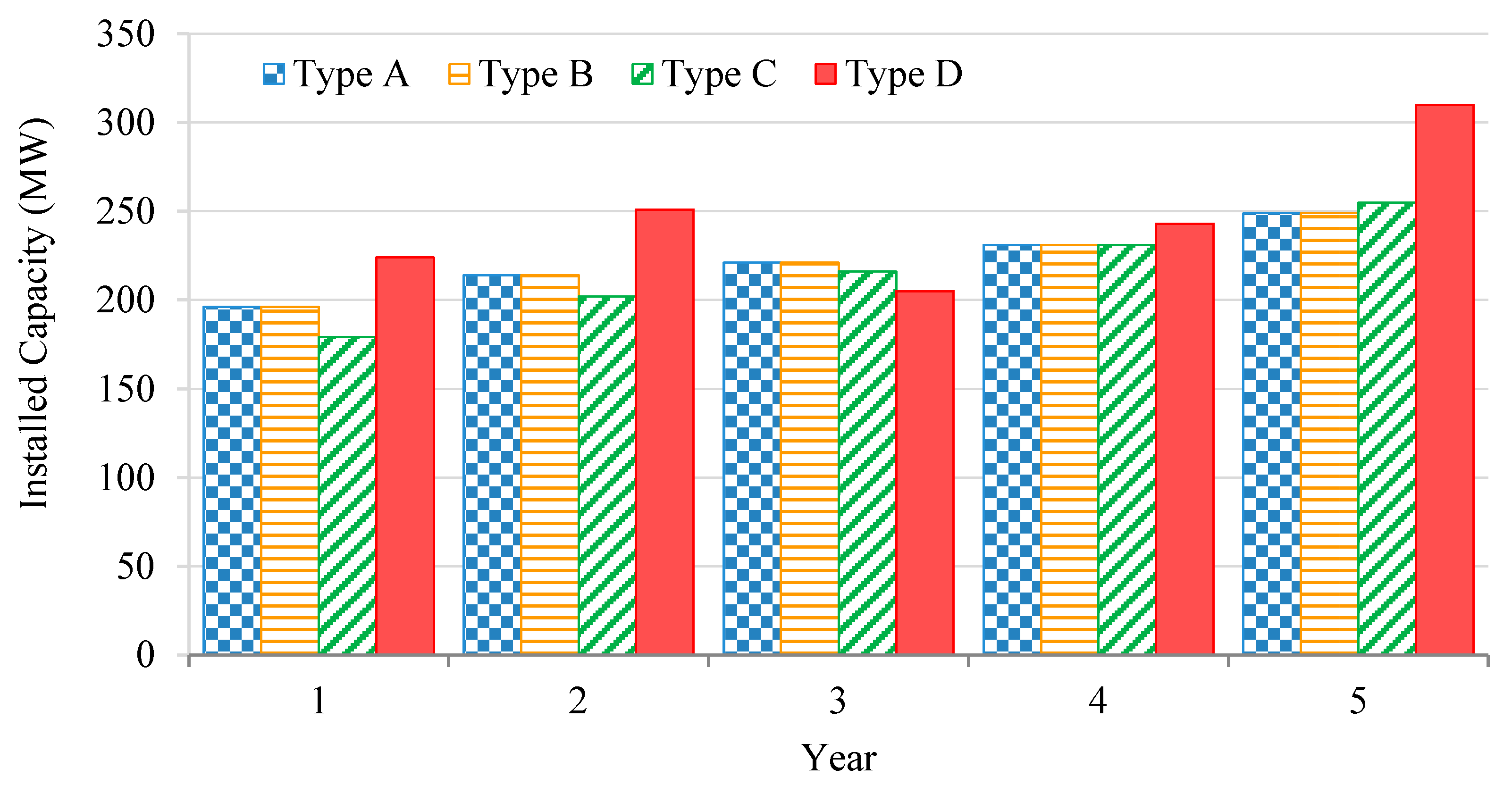
The GEP strategy of the least capacity is sought under the assumption that the smaller the installed capacity, the lower the cost. The installed capacity at which the NLCC is equal to the load growth is selected as the optimal value every year. The total installed capacities of all unit types during the whole period are listed in Table 6. The value of the total installed capacity of a certain type represents the extent to which the units of that type contribute to flexibility during the period. The larger the total installed capacity of a given type, the smaller the NLCC of that type. As expected from the results in Scenarios 1 and 2, the optimal value is achieved using type C, which has the lowest priority in the merit order and the largest ramp rate. It is also observed that when the ramp rate is high (low), the total installed capacity is small (large), as the priority is lower. This means that utilizing a fast unit (slow unit) as a reserve unit (power-loading unit) rather than a power-loading unit (reserve unit) is more effective in terms of flexibility.
The installed capacities of every unit type for every year are also shown in Figure 6. For those of high priority (i.e., type A and type B), there is no difference according to ramp rate; all the type-A and type-B units are committed into operation and also maintain the operating points over a certain level, at which the ramp rate does not affect the NLCC. Meanwhile, type C and type D belong to the low-priority types. As both types have the same priority in the merit order, they obtain the same scheduling results. However, there is quite a difference between type C and type D in regards to the annual increment. Unlike type C, type D shows irregular variations in the annual increment, which is due to the relationship between the ramp rate of each type and the ramping capability requirement each year.
5. Conclusions
This paper proposed a concept of NLCC to evaluate the contribution of a generating unit to the flexibility of a power system, which is defined as the ability to respond to changes in net load. The NLCC is defined as the amount by which the load can be increased while maintaining the same flexibility (as measured by RSE) when the unit is added to the system. This index is based on the RSE flexibility index, which has been used to capture the risk for flexibility. Compared to ELCC, the NLCC index is more adequate to evaluate the contribution of a generating unit to the system flexibility, because it takes into consideration the operating conditions, such as operating point and ramp rate. With a modified IEEE-RTS-96, a case study has been conducted to verify the applicability of the method. The simulation results show the impact of the operating conditions on the NLCC and reveal which kind of unit is more effective in terms of flexibility. As part of future work, it would be interesting to apply the NLCC index to the GEP of the Korean power system. We also plan to evaluate the impact of network constraint and demand side resource on the NLCC.
Acknowledgments
This research was supported by Korea Electric Power Corporation through Korea Electrical Engineering & Science Research Institute (grant number: R15XA03-55) and Basic Science Research Program through the National Research Foundation of Korea (NRF) funded by the Ministry of Education (2017R1D1A1B03029308).
Author Contributions
Chang-Gi Min carried out the main body of research and Mun-Kyeom Kim reviewed the work continuously.
Conflicts of Interest
The authors declare no conflict of interest.
Nomenclature
| Ai,t | Random variable representing availability of unit i at time t (1 if available, 0 otherwise) |
| c | Element of Ct−Δt |
| Ct−Δt | Set of combination of Ai,t−Δt when Oi,t−Δt is non-zero for all i |
| e | Element of Et−Δt |
| Et−Δt | Set of NLFEt |
| FNLt | Forecast net load at time t |
| i | Index of generating unit |
| I | Set of generating unit |
| LOLPt | Loss of load probability at time t |
| NLFEt | Random variable representing net load forecast error at time t |
| Oi,t | Value representing whether unit i is on-line at time t |
| OCs,t | Outage capacity of failure scenario s at time t |
| Pi,t | Generation output of unit i at time t |
| Pmax,i | Maximum generation level of unit i |
| Prob(·) | Probability in the brackets. |
| Probc[·] | Probability of c if condition [∙] is satisfied, 0 otherwise. |
| RCRt | Ramping capability requirement at time t |
| rri | Ramp rate of unit i |
| RSPt | Ramping capability shortage probability at time t |
| s | Index of failure scenario |
| SRCt | System ramping capability at time t |
| t | Index of time |
| Δt | Minimum time interval between operating points |
Appendix A. ELCC Calculation for the Example in Section 3
Appendix A.1. Calculation Procedure of ELCC
Step 1: Calculate the LOLE for the system before the unit is added.
Step 2: Change the net load and calculate the LOLE with changes in the net load.
Step 3: Add a new unit into the system. Change the net load, while keeping all other data fixed, and calculate the LOLE.
Step 4: The difference between the net load level at the LOLE criterion in Step 2 and that in Step 3 is ELCC.
Appendix A.2. ELCC for the Example
Step 1: Based on the Markov chain-based capacity state model, the failure probabilities of all units are calculated as at 0 h, at 1 h, and at 2 h. The outage probabilities for different failure cases are presented in Table A1. For example, the probability that all units are available at 0 h is calculated as . The LOLPt is the sum of the probabilities that outage capacity is non-zero at time t, and it is represented by:
The LOLP0 is equal to because an outage event occurs only when the number of failed units is three; that is,
A LOLE of h/period is derived by adding all LOLPt. This value is also chosen as the LOLE criterion (For reference, the unit of LOLE, in principle, varies with the targeted period, which here corresponds to 3 h).

Table A1.
Outage probability of a system without Unit D.
| # of Failed Unit | Avail. Capacity (MW) | Outage Capacity at 0 h (MW) | Outage Capacity at 1 h (MW) | Outage Capacity at 2 h (MW) | Prob. at 0 h & 2 h | Prob. at 1 h |
|---|---|---|---|---|---|---|
| 0 | 300 | 0 | 0 | 0 | ||
| 1 | 200 | 0 | 0 | 0 | ||
| 2 | 100 | 0 | 0 | 50 | ||
| 3 | 0 | 50 | 50 | 150 |
Step 2: The load level is varied within a range from 0% to 50% with a step size of 5%, and the LOLE for the load variances are then calculated, as shown in Table A2.
Table A2.
Loss of load expectation (LOLE) for load variances of system without Unit D.
| Load Variance (%) | Load Level at 0 h/1 h/2 h (MW) | LOLP0 | LOLP1 | LOLP2 | LOLE (=LOLP0 + LOLP1 + LOLP2) (h/period) |
|---|---|---|---|---|---|
| 0 | 50/50/150 | ||||
| 5 | 52.5/52.5/157.5 | ||||
| 10 | 55/55/165 | ||||
| 15 | 57.5/57.5/172.5 | ||||
| 20 | 60/60/180 | ||||
| 25 | 62.5/62.5/187.5 | ||||
| 30 | 65/65/195 | ||||
| 35 | 67.5/67.5/202.5 | ||||
| 40 | 70/70/210 | ||||
| 45 | 72.5/72.5/217.5 | ||||
| 50 | 75/75/225 |
Step 3: Unit D is added to the system, and the outage probabilities for four generating units are obtained, as listed in Table A3. The LOLE for the load variances are also computed, as shown in Table A4.
Table A3.
Outage probability of a system with Unit D.
| # of Failed Unit | Available Capacity (MW) | Outage Capacity at 0 h (MW) | Outage Capacity at 1 h (MW) | Outage Capacity at 2 h (MW) | Prob. at 0 h & 2 h | Prob. at 1 h |
|---|---|---|---|---|---|---|
| 0 | 400 | 0 | 0 | 0 | ||
| 1 | 300 | 0 | 0 | 0 | ||
| 2 | 200 | 0 | 0 | 0 | ||
| 3 | 100 | 0 | 25 | 100 | ||
| 4 | 0 | 100 | 125 | 200 |
Table A4.
LOLE for load variances of a system with Unit D.
| Load Variance (%) | Load Level at 0 h/1 h/2 h (MW) | LOLP0 | LOLP1 | LOLP2 | LOLE (=LOLP0 + LOLP1 + LOLP2) (h/period) |
|---|---|---|---|---|---|
| 0 | 50/50/150 | ||||
| 5 | 52.5/52.5/157.5 | ||||
| 10 | 55/55/165 | ||||
| 15 | 57.5/57.5/172.5 | ||||
| 20 | 60/60/180 | ||||
| 25 | 62.5/62.5/187.5 | ||||
| 30 | 65/65/195 | ||||
| 35 | 67.5/67.5/202.5 | ||||
| 40 | 70/70/210 | ||||
| 45 | 72.5/72.5/217.5 | ||||
| 50 | 75/75/225 |
Step 4: The LOLE begins to exceed the LOLE criterion when the load variance is 35%. In order to find a point coinciding with the LOLE criterion, the load variances are increased by 1% in each step from 30% to 35%, and the corresponding LOLE are derived. The changing point occurs when the load variance is 34%; thus, in this example, the ELCC is equal to the peak load multiplied by 33%; that is, 49.5 MW.
Appendix B. Failure and Repair Rates in Case Study
Table A5.
Failure and repair rates of 26 generating units.
| Unit # | Failure Rate (occurrences/h) | Repair Rate (occurrences/h) |
|---|---|---|
| 1–5 | 1/2940 | 1/60 |
| 6–9 | 1/450 | 1/50 |
| 10 | 1/1960 | 1/40 |
| 11, 12 | 1/450 | 1/40 |
| 13 | 1/1960 | 1/40 |
| 14–16 | 1/1200 | 1/50 |
| 17–20 | 1/960 | 1/40 |
| 21–23 | 1/950 | 1/50 |
| 24 | 1/1150 | 1/100 |
| 25, 26 | 1/1100 | 1/150 |
References
- Huber, M.; Dimkova, D.; Hamacher, T. Integration of wind and solar power in Europe: Assessment of flexibility requirements. Energy 2014, 69, 236–246. [Google Scholar] [CrossRef]
- Lund, P.D.; Lindgren, J.; Mikkola, J.; Salpakari, J. Review of energy system flexibility measures to enable high levels of variable renewable electricity. Renew. Sustain. Energy Rev. 2015, 45, 785–807. [Google Scholar] [CrossRef]
- Mathiesen, B.V.; Lund, H.; Connolly, D.; Wenzel, H.; Østergaard, P.A.; Möller, B.; Nielsen, S.; Ridjan, I.; Karnøe, P.; Sperling, K. Smart Energy Systems for coherent 100% renewable energy and transport solutions. Appl. Energy 2015, 145, 139–154. [Google Scholar] [CrossRef]
- Spiecker, S.; Weber, C. The future of the European electricity system and the impact of fluctuating renewable energy—A scenario analysis. Energy Policy 2014, 65, 185–197. [Google Scholar] [CrossRef]
- Navid, N.; Rosenwald, G. Ramp Capability Product Design for MISO Markets; MISO: Carmel, IN, USA, 2013. [Google Scholar]
- Zhao, J.; Zheng, T.; Litvinov, E. A unified framework for defining and measuring flexibility in power system. IEEE Trans. Power Syst. 2015, 99, 1–9. [Google Scholar] [CrossRef]
- Deane, J.; Drayton, G.; Gallachóir, B.Ó. The impact of sub-hourly modelling in power systems with significant levels of renewable generation. Appl. Energy 2014, 113, 152–158. [Google Scholar] [CrossRef]
- Kubik, M.; Coker, P.J.; Barlow, J.F. Increasing thermal plant flexibility in a high renewables power system. Appl. Energy 2015, 154, 102–111. [Google Scholar] [CrossRef]
- Moiseeva, E.; Wogrin, S.; Hesamzadeh, M.R. Generation flexibility in ramp rates: Strategic behavior and lessons for electricity market design. Eur. J. Oper. Res. 2017, in press. [Google Scholar] [CrossRef]
- Oree, V.; Hassen, S.Z.S. A composite metric for assessing flexibility available in conventional generators of power systems. Appl. Energy 2016, 177, 683–691. [Google Scholar] [CrossRef]
- Belderbos, A.; Delarue, E. Accounting for flexibility in power system planning with renewables. Int. J. Electr. Power Energy Syst. 2015, 71, 33–41. [Google Scholar] [CrossRef] [Green Version]
- Brouwer, A.S.; van den Broek, M.; Seebregts, A.; Faaij, A. Operational flexibility and economics of power plants in future low-carbon power systems. Appl. Energy 2015, 156, 107–128. [Google Scholar] [CrossRef]
- Koltsaklis, N.E.; Georgiadis, M.C. A multi-period, multi-regional generation expansion planning model incorporating unit commitment constraints. Appl. Energy 2015, 158, 310–331. [Google Scholar] [CrossRef]
- Pereira, S.; Ferreira, P.; Vaz, A. Generation expansion planning with high share of renewables of variable output. Appl. Energy 2017, 190, 1275–1288. [Google Scholar] [CrossRef]
- Koltsaklis, N.E.; Liu, P.; Georgiadis, M.C. An integrated stochastic multi-regional long-term energy planning model incorporating autonomous power systems and demand response. Energy 2015, 82, 865–888. [Google Scholar] [CrossRef]
- Mejía-Giraldo, D.; McCalley, J.D. Maximizing future flexibility in electric generation portfolios. IEEE Trans. Power Syst. 2014, 29, 279–288. [Google Scholar] [CrossRef]
- Santos, M.J.; Ferreira, P.; Araújo, M. A methodology to incorporate risk and uncertainty in electricity power planning. Energy 2016, 115, 1400–1411. [Google Scholar] [CrossRef]
- Krishnan, V.; Das, T.; Ibanez, E.; Lopez, C.A.; McCalley, J.D. Modeling operational effects of wind generation within national long-term infrastructure planning software. IEEE Trans. Power Syst. 2013, 28, 1308–1317. [Google Scholar] [CrossRef]
- Lannoye, E.; Milligan, M.; Adams, J.; Tuohy, A.; Chandler, H.; Flynn, D.; O’Malley, M. Integration of variable generation: Capacity value and evaluation of flexibility. In Proceedings of the 2010 IEEE Power and Energy Society General Meeting, Detroit, MI, USA, 25–29 July 2010; pp. 1–6. [Google Scholar]
- Min, C.G.; Park, J.K.; Hur, D.; Kim, M.K. A risk evaluation method for ramping capability shortage in power systems. Energy 2016, 113, 1316–1324. [Google Scholar] [CrossRef]
- Garver, L.L. Effective load carrying capability of generating units. IEEE Trans. Power App. Syst. 1966, PAS-85, 910–919. [Google Scholar] [CrossRef]
- Abdullah, M.A.; Muttaqi, K.M.; Agalgaonkar, A.P.; Sutanto, D. A noniterative method to estimate load carrying capability of generating units in a renewable energy rich power grid. IEEE Trans. Sustain. Energy 2014, 5, 854–865. [Google Scholar] [CrossRef]
- Tan, Y.; Meegahapola, L.; Muttaqi, K.M. A review of technical challenges in planning and operation of remote area power supply systems. Renew. Sustain. Energy Rev. 2014, 38, 876–889. [Google Scholar] [CrossRef]
- Milligan, M.; Frew, B.; Zhou, E.; Arent, D.J. Advancing System Flexibility for High Penetration Renewable Integration; NREL: Golden, CO, USA, 2015.
- Milligan, M.; Porter, K. The capacity value of wind in the United States: Methods and implementation. Electr. J. 2006, 19, 91–99. [Google Scholar] [CrossRef]
- Wangdee, W.; Billinton, R. Considering load-carrying capability and wind speed correlation of WECS in generation adequacy assessment. IEEE Trans. Energy Convers. 2006, 21, 734–741. [Google Scholar] [CrossRef]
- Finon, D.; Pignon, V. Electricity and long-term capacity adequacy: The quest for regulatory mechanism compatible with electricity market. Util. Policy 2008, 16, 143–158. [Google Scholar] [CrossRef]
- Billinton, R.; Karki, R.; Gao, Y.; Huang, D.; Hu, P.; Wangdee, W. Adequacy assessment considerations in wind integrated power systems. IEEE Trans. Power Syst. 2012, 27, 2297–2305. [Google Scholar] [CrossRef]
- Chen, Z.; Wu, L.; Shahidehpour, M. Effective load carrying capability evaluation of renewable energy via stochastic long-term hourly based SCUC. IEEE Trans. Sustain. Energy 2015, 6, 188–197. [Google Scholar] [CrossRef]
- Min, C.G.; Kim, M.K. Flexibility-Based Evaluation of Variable Generation Acceptability in Korean Power System. Energies 2017, 10, 825. [Google Scholar]
- Billinton, R.; Allan, R. Reliability Evaluation of Power Systems, 2nd ed.; Springer Science & Business Media: New York, NY, USA, 2013. [Google Scholar]
- Keane, A.; Milligan, M.; Dent, C.J.; Hasche, B.; D’Annunzio, C.; Dragoon, K.; Holttinen, H.; Samaan, N.; Soder, L.; O’Malley, M. Capacity value of wind power. IEEE Trans. Power Syst. 2011, 26, 564–572. [Google Scholar] [CrossRef] [Green Version]
- Wood, A.J.; Wollenberg, B.F. Power Generation, Operation, and Control, 3rd ed.; John Wiley & Sons: Hoboken, NJ, USA, 2012. [Google Scholar]
Figure 1.
Result of generation schedule.

Figure 2.
A case of load-shedding.

Figure 3.
Forecasted net load profile.

Figure 4.
RSE before and after adding a 400-MW unit.

Figure 5.
RSE before and after adding a 100-MW unit.

Figure 6.
Installed capacities of each type unit for every year.

Table 1.
Load-shedding result and consequential RSPt (Y: Yes, N: No).
| Failure Cases | Load Shedding or not at 1 h/2 h | Prob. at 0 h | Prob. at 1 h |
|---|---|---|---|
| - | N/N | ||
| A | N/Y | ||
| B | N/Y | ||
| C | N/N | ||
| A&B | N/Y | ||
| A&C | N/Y | ||
| B&C | N/Y | ||
| A&B&C | Y/Y | ||
| - | RSP1: | RSP2: | |
Table 2.
Ramping capability shortage expectation (RSE) for load variances of system without Unit D.
| Load Variance (%) | RSP1 | RSP2 | RSE (=RSP1 + RSP2) (h/period) |
|---|---|---|---|
| 0 | |||
| 5 | |||
| 10 | |||
| 15 | |||
| 20 | |||
| 25 | |||
| 30 | |||
| 35 | |||
| 40 | |||
| 45 | |||
| 50 |
Table 3.
RSE for load variances of system with Unit D.
| Load Variance (%) | RSP1 | RSP2 | RSE (=RSP1 + RSP2) (h/period) |
|---|---|---|---|
| 0 | |||
| 5 | |||
| 10 | |||
| 15 | |||
| 20 | |||
| 25 | |||
| 30 | |||
| 35 | |||
| 40 | |||
| 45 | |||
| 50 |
Table 4.
Load growth scenario.
| Year | Peak Load (MW) | Load Growth (MW) |
|---|---|---|
| 0 | 2531 | - |
| 1 | 2708.025 | 177 |
| 2 | 2897.587 | 190 |
| 3 | 3100.418 | 203 |
| 4 | 3317.447 | 217 |
| 5 | 3549.668 | 232 |
Table 5.
Four types of generating unit for generation expansion planning (GEP).
| Unit Type | Rating (MW) | Priority in Merit Order | Ramp Rate (% of rating/h) |
|---|---|---|---|
| A | 0–400 | High | 100 |
| B | 0–400 | High | 80 |
| C | 0–400 | Low | 100 |
| D | 0–400 | Low | 80 |
Table 6.
Total installed capacity of four types of unit.
| Unit Type | A | B | C | D |
|---|---|---|---|---|
| Total installed capacity (MW) | 1111 | 1111 | 1083 | 1233 |
© 2017 by the authors. Licensee MDPI, Basel, Switzerland. This article is an open access article distributed under the terms and conditions of the Creative Commons Attribution (CC BY) license (http://creativecommons.org/licenses/by/4.0/).
Share and Cite
MDPI and ACS Style
Min, C.-G.; Kim, M.-K. Net Load Carrying Capability of Generating Units in Power Systems. Energies 2017, 10, 1221. https://doi.org/10.3390/en10081221
AMA Style
Min C-G, Kim M-K. Net Load Carrying Capability of Generating Units in Power Systems. Energies. 2017; 10(8):1221. https://doi.org/10.3390/en10081221
Chicago/Turabian StyleMin, Chang-Gi, and Mun-Kyeom Kim. 2017. "Net Load Carrying Capability of Generating Units in Power Systems" Energies 10, no. 8: 1221. https://doi.org/10.3390/en10081221
Note that from the first issue of 2016, this journal uses article numbers instead of page numbers. See further details here.