Optimal Power Flow Using Particle Swarm Optimization of Renewable Hybrid Distributed Generation


1
Electrical Engineering Department, College of Engineering, King Saud University, P.O. Box. 800, Riyadh 11421, Saudi Arabia
2
Electrical Engineering Department, Faculty of Energy Engineering, Aswan University, Aswan Governorate 81528, Egypt
3
Electrical Engineering Department, Mansoura University, Mansoura 35516, Egypt
4
Sustainable Energy Technology Center, King Saud University, Riyadh 11421, Saudi Arabia
5
Ecole Centrale de Lyon, University of Lyon, Ampere CNRS UMR 5005, 36 avenue Guy Collongue, Ecully 69134, France
*
Author to whom correspondence should be addressed.
Energies 2017, 10(7), 1013; https://doi.org/10.3390/en10071013
Submission received: 16 May 2017
/
Revised: 7 July 2017
/
Accepted: 10 July 2017
/
Published: 17 July 2017
(This article belongs to the Section F: Electrical Engineering)
Abstract
:The problem of voltage collapse in power systems due to increased loads can be solved by adding renewable energy sources like wind and photovoltaic (PV) to some bus-bars. This option can reduce the cost of the generated energy and increase the system efficiency and reliability. In this paper, a modified smart technique using particle swarm optimization (PSO) has been introduced to select the hourly optimal load flow with renewable distributed generation (DG) integration under different operating conditions in the 30-bus IEEE system. Solar PV and wind power plants have been introduced to selected buses to evaluate theirs benefits as DG. Different solar radiation and wind speeds for the Dammam site in Saudi Arabia have been used as an example to study the feasibility of renewable energy integration and its effect on power system operation. Sensitivity analysis to the load and the other input data has been carried out to predict the sensitivity of the results to any deviation in the input data of the system. The obtained results from the proposed system prove that using of renewable energy sources as a DG reduces the generation and operation cost of the overall power system.
1. Introduction
Optimal power flow (OPF) studies aim to optimize specific objectives by adjusting some power system variables, provided that all equality and inequality constraints of the system are satisfied. Based on its energy management capability, OPF became one of the most important areas of study in the electric power field. OPF is a highly constrained and nonlinear problem with continuous and discrete variables. In 1962, Huneault et al. [1] published the first paper on OPF. Since then, researchers started studying the OPF problem extensively. The methods or techniques that have been implemented to optimize the OPF are divided into two categories: deterministic methods and evolutionary methods. Deterministic methods include linear [2] and nonlinear programming (LP) [3], quadratic programming (QP) [4], and interior point method (IM) [5]. These methods have a problem in handling many local minima due to the non-convexity of OPF problems. Gradient-based methods overcome the convergence problem, but sometime fail to meet inequality constraints [6]. Due to the limitations of deterministic methods, evolutionary methods were introduced to remedy these limitations and optimize OPF problems effectively. Evolutionary methods include genetic algorithm (GA) [7,8], evolutionary programming (EP) [9], particle swarm optimization (PSO) [10,11], simulated annealing (SA) [12], differential algorithm (DE) [13], and shuffle frog leaping algorithm (SFLA) [14]. These methods have been discussed in details in [15]. Some researchers have even tried to hybridize the two methods in OPF to improve the performance of the optimization technique to reach the global solution easier and faster. Roy et al. [16] used a modified SFLA with GA in solving economic load dispatch problems. Other researchers used chaos optimization with linear IM method [17]. GA with fuzzy logic was also implemented and has been used for OPF solution in [18]. A hybrid method of PSO, GA and fuzzy logic techniques was also used in OPF [19].
The allocation of distributed generation (DG) is another interesting area of research. GA was used to optimize the allocation of dispersed generation resources in distribution networks [20]. A technique for selecting the buses in a sub-transmission system to optimally locate DG has been proposed to reduce transmission losses [21] which can be translated into reductions in total energy cost. Most OPF studies use systems with constant loads or study a certain load and generation case. Variable loads have been considered in [22,23,24] to study the effect of varying loads or load expansion on the operation of the power system.
Integration of renewable energy sources in power systems has many benefits, such as reducing greenhouse emissions, especially CO2 emissions, and hence assisting in resolving the global warming problem, and reducing the power losses in transmission lines due to power transferring from remote areas. However, the capital cost of renewable power plants is very high compared to conventional power plants, although conversely the operation and maintenance costs are cheaper than those for conventional generation and will continue to decline with recent technical developments.
Since most renewable resources are intermittent in nature, it is advantageous to utilize more than one resource when available. Hybridizing renewable resources improves the power system reliability, efficiency and economy. Hybrid renewable energy systems (HRES) can be standalone power systems or integrated with conventional generation [25,26,27,28,29]. Economic modeling of HRES was also conducted in [26], which proved the feasibility of installing HRES.
This paper presents an OPF study of a power system integrated with distributed wind and solar PV as a renewable DG. A modified PSO (MPSO) algorithm is applied to the 30 bus IEEE system with variable load to assess the benefits from using REDG in power systems. The simulation program using MPSO shows the ability to reach the global minimum solution faster and more accurately than with other techniques [30,31]. The results also show considerable reductions in cost and transmission line losses in case of using renewable energy sources as a DG.
1.1. Particles Swarm Optimization Technique
PSO is smart optimization technique that has been used in many applications. This was first introduced to scientific community by Eberhart and Kennedy [32]. As shown in this paper, this optimization technique is an adaptive algorithm based on a social-psychological metaphor; a population of individuals (referred to as particles) adapts by returning stochastically toward previously successful regions. In this technique a velocity and position should be updated continually. During each iteration, each particle is accelerated toward the particle’s previous best position and the global best position. Under each iteration, the particle position will be updated using the new velocity which is counted as the distance from its previous best position, and the distance from the global best position will be calculated. The new velocity of each particle will be used to calculate the next position of the particle in the search space. This process will be repeated again for number of iterations until a minimum error is achieved [33].
The velocity and position of each particle during the PSO optimization steps are shown in Equations (1) and (2) [32]:
where, c1 and c2 are constants in the range from 0 to 4 and has been used as 2 in this paper, ω is the inertia, r1, r2 are random variables which are uniformly distributed between 0 to 1, pg is the global best position, xij is current position, pij the best position for the current particle and vij is the velocity of particles. j is the counter for iteration number, and i is the counter for particle number.
The pseudo code of the procedure is as follows [34]:
Begin;
Generate random population of N solutions (particles);
For each individual i ϵ N: calculate fitness (i); where N is the total number of particles.
Initialize the value of the weight factor, ω;
For each particle;
Set pBest as the best position of particle i;
If fitness (i) is better than pBest;
pBest = fitness (i);
End;
Set gBest as the best fitness of all particles;
For each particle;
Calculate particle velocity according to Equation (1);
Update particle position according to Equation (2);
End; Update the value of the weight factor, ω;
Check if termination = true;
1.2. Optimal Power Flow Formulation
OPF is generally formulated mathematically using compact notation as follows [35]:
with nonlinear equality constraints:
and inequality constraints:
where, F(u, x) is the objective function which should be minimized (or maximized); G (x, u) represents the power flow nonlinear equations; H(u, x) represents various limits of the system control variables like generators power limits, bus voltages limits and lines limits; u is a vector of the system controlled variables like generators voltage, generators active power, transformers tap settings and shunt VAR compensations, load M and Mega Volt-Ampere Reactive MVAR (load shedding), dc power transmission; x is a vector of dependent variables that includes slack bus power, load bus voltages magnitude and phase angles, generator reactive power outputs for bus voltage control, reference bus voltage magnitude and angle (fixed) and transmission lines parameters.
minimize F(x, u)
G (x, u) = 0
H (x, u) < 0
umin < u < umax
xmin < x < xmax
1.3. Fuel Cost Objective Function
Total generation fuel cost function which is the objective function in this study is expressed as shown in the following equation [36]:
where, γ, β and α are the cost function coefficients; and NG is number of generators. For a particular load the total generation cost should be minimum. The equality nonlinear constraints are given by the following equations:
where, the active and reactive power generation at bus-bar i (Pi and Qi) can be obtained from the following equations:
where, Vi and Vj are the buses voltages of busbars i and j, respectively. , are the angles of ith, and jth bus-bars, respectively, Yij is the admittance between buses i and j, is the admittance angle of , and NB is number of buses.
At any time, the total generation must meet the total load plus the transmission losses as shown in the following equation:
where, ND is the number of load buses, NG is the number of generator buses, PGi and PDi are the generation power and load power at bus-bar i, and PL is the total transmission losses.
The above equations must be solved with the following generators constraints:
where, Pmin and Pmax are the minimum and maximum active power constraints for each generator, respectively. Qmin and Qmax are the minimum and maximum reactive power constraints for each generator, respectively. Vmin and Vmax are the minimum and maximum voltage magnitude constraints for each bus. δmin and δmax are the minimum and maximum voltage angle constraints for each bus, respectively.
1.4. Wind and Solar Energy Modeling
The wind power generated by wind turbines is calculated using the following equation [37]:
where, is the air density in kg/m3, A is the rotor swept area in m2, Cp is the turbine coefficient of performance (The theoretical value of Cp is 59.3%), w is the wind speed at hub position m/s, Nt is number of turbines and η is the net efficiency of wind turbine. However, the modern turbines reached a value of 50% [38]. In this paper the coefficient of performance has been used as 45% except in sensitivity analysis showing its effect on the total cost.
The solar energy is calculated using the following equation:
where, I is the solar radiation in W/m2, Ap is the panel area, Np is the number of panels, and ηp is the panels’ efficiency.
2. System Description
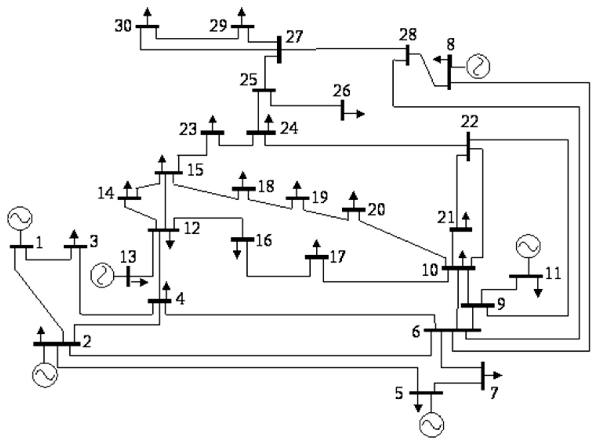
This paper studies the OPF problem in the case of integration of renewable energy generations with the power system as DG. The study was applied on the IEEE 30-bus system as shown in Figure 1. A full description of this system’s components can be found in [39]. Variable loads at the system buses were assumed. Four renewable energy power plants are inserted into the power system, mainly, two wind energy power plants and two solar energy power plants. Two wind energy power plants are inserted at buses 7 and 12 with 250 wind turbines at each wind farm. Two solar PV power plants are inserted at buses 8 and 18. The number of the PV panels is 40,000 and 380,000, respectively. The total capacity of the renewable power was chosen so that it represents 10% of the conventional generation to avoid technical problems [40,41]. The wind speed and solar radiation are assumed variable and different at each location of renewable generation power plant to be flexible when using this strategy in any real power system.
The system consists of six generators at buses 1, 2, 5, 8, 11 and 13. The Newton-Raphson method has been used in calculating the load flow equations of the power system at each time point. The PSO algorithm was implemented to find the optimal generation scheduling under variable load and renewable generation for certain period of time (24 h to represent a day has been used in this study).
The selection of these buses for integration of renewable energy generation is based on selecting a bus that is connected to other loaded buses. The idea behind this is to locate the renewable energy power plants near load centers to minimize the transmission losses. Both wind speed and solar radiation are assumed different at each bus to provide more flexibility to the proposed program. The wind speed, solar radiation, and the loads of the system buses are varied over a 24 h period to simulate the actual real time scenarios for one day. The data of wind speed and solar radiation were obtained from the Dammam site at Saudi Arabia as an example. This enables us to predict the dynamic performance of the power system in terms of economics and technical point of views. The operation and maintenance cost (O&M) of wind energy has been taken as 1.655 $/MWh for PV systems [42]. For wind the O&M cost is taken as 2.250 $/MWh [43]. The commercially available SM100 PV array (Siemens, Munich, Germany) has been considered in the design of 10 kW PV system with 15% efficiency. The electric characteristics of this PV module are rated power of 100 W, rated voltage of 34 V, rated current of 2.95 A, nominal temperature of 20 °C, and rated saturation current of 0.00405 A. The PV array consists of several modules in series (Ns) and parallel rows (Np).
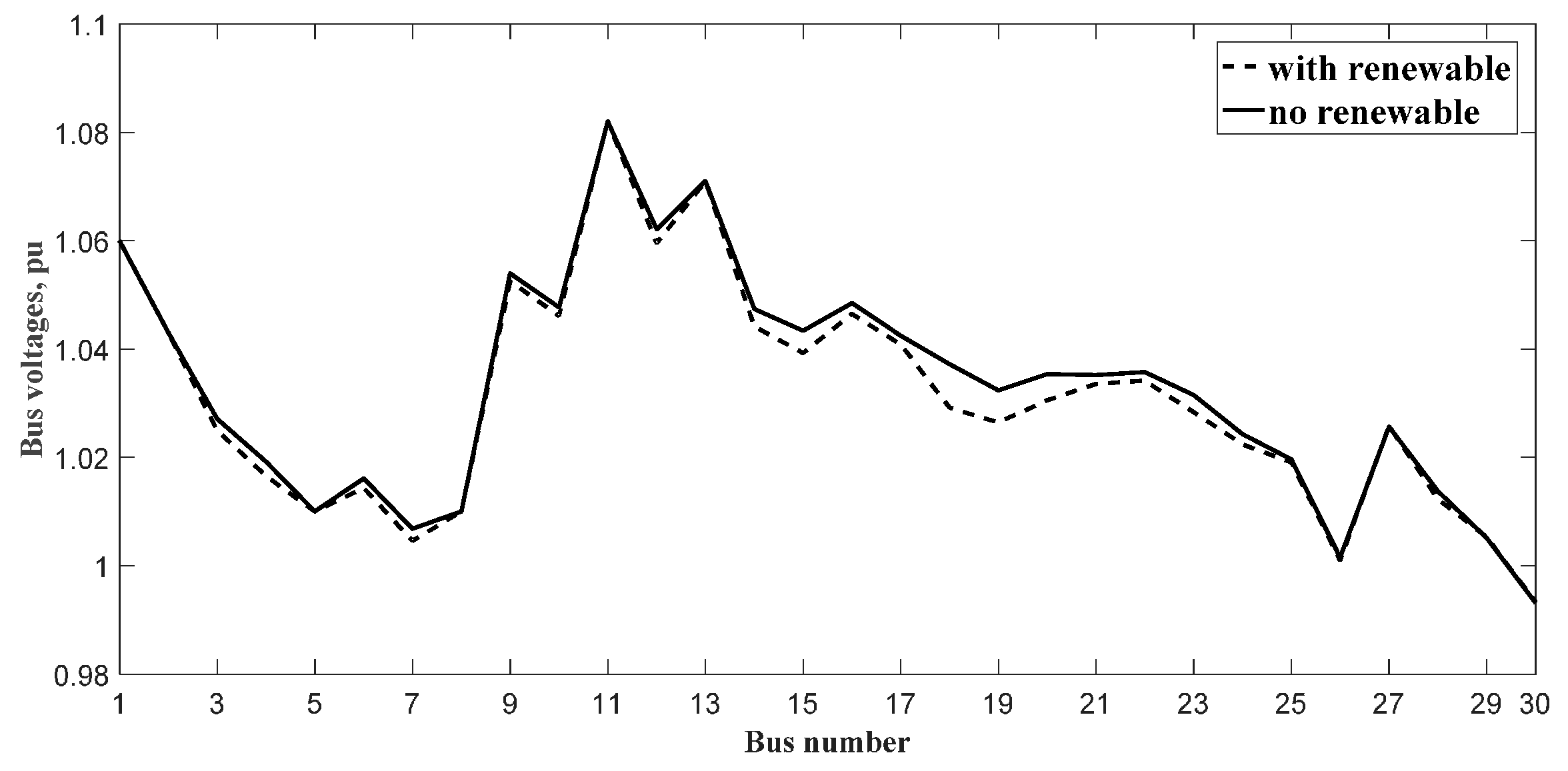
To check the suitability of the selected buses for integration of renewable energy sources, the buses’ voltage magnitude can be investigated. Figure 2 shows the buses’ voltage magnitude for the base case without renewable sources and for the system with integration of renewable energy sources. It’s clear from this figure that the deviation of buses’ voltage magnitude from 1 p.u. decreased after the integration of the renewable energy sources at buses 7, 8, 12 and 18. Therefore, the selection of the buses 7, 8, 12 and 18 for integration of renewable energy sources shows an improvement in voltage stability.
Validation
To validate this work, the results of the base case which is the base load without integrating renewable energy power plants will be compared with results reported in the literature. The total load of the original 30 bus IEEE system is 283.4 MW. The total generation cost at that load is 801.8 $/h according to our model. Table 1 [19] shows different values found in the literature. One notes that our result is quite consistent with those results which give a validation of the work done in this paper.
3. Results and Discussion
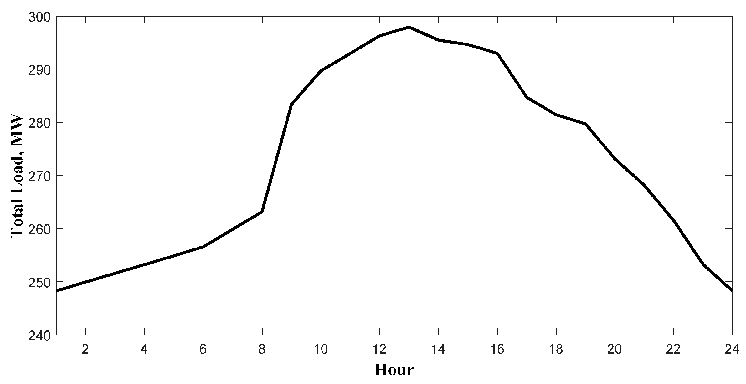
The total load of the system is shown in Figure 3 for 24 h. The peak load occurs at midday and the maximum load is 283.1 MW at hour 13.
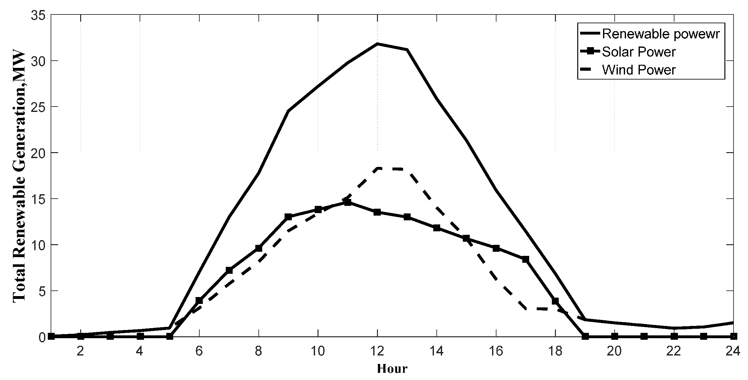
The renewable energy generation over the 24 h period is shown in Figure 4. The total generated power from solar panels, the total wind power generation, and the total renewable generation which is the sum of solar PV power and wind power generation are illustrated in Figure 4. Maximum PV power occurs at hour 11. Usually, solar radiation is maximum at the hour 12, but sometimes cloud and dust reduce the radiation reaching the PV panels level at a particular time. This explains the shape of solar PV power generation curve shown in Figure 4. The wind power generation curve could have any shape according to the wind speed. It may be like constant with little or large fluctuations or it may be intermittent with very low values at some hours and high values at others. Here in this paper, the wind power generation has its peak amplitude between the hours 12 and 13. A good feature in the total renewable energy production is the correlation between the generated power from renewable energy sources with the electric loads as shown in Figure 3 and Figure 4. This helps in extending the total power generation capacity of the system and meeting the extra demand without installing new conventional fuel power plants. The maximum total renewable power generation is 31.8 MW at time 12, which represents 10.3% of the conventional fuel power generation.
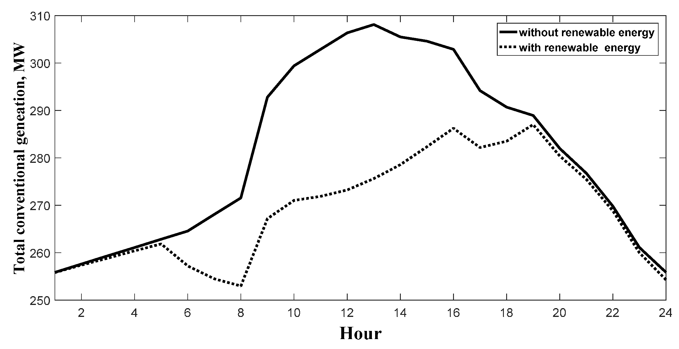
3.1. Total Conventional Generation
The total conventional generation of the system with and without renewable energy generation integration is shown in Figure 5. This figure illustrates that the renewable energy system provides the power to the load at peak time which explains the correlation between the generation and the load from renewable energy system which presents its superiority to be used in the power system as a DG. This figure shows a significant reduction in conventional generation and hence, fossil fuel saved when renewable energy generation is integrated. The availability of renewable energy in the peak load period decreases the generators loading in these times. The peak of generators loading is shifted from midday hours, between hours 16–19, in this case. The availability of solar power during peak load period will definitely decrease of generators’ loading, but wind speed may contribute at any time during the day. Therefore, different generators’ loading curves or shapes will be produced. During the early and late hours, the two curves are close to each other. This is because of low contribution from renewable energy during these periods.
Furthermore, there are different incremental rates in conventional generation over the 24 h. During the hours between 1 and 10, the incremental rate is linear while it is closer to nonlinear between 10 and 19. This change in the increment rate is due to the simultaneous change in load demand and renewable energy generation. In the hours between 16 and 19, there is a slight decrease in conventional generation followed by obvious increase. These trends in few hours may occur in power systems integrated with renewable generation. However, this represents undesirable behavior in power systems and introduces big challenge in the operation and control of such power systems.
Further studies should focus on studying this phenomenon to overcome such a technical problem and others associated with integrating renewable energy generation.
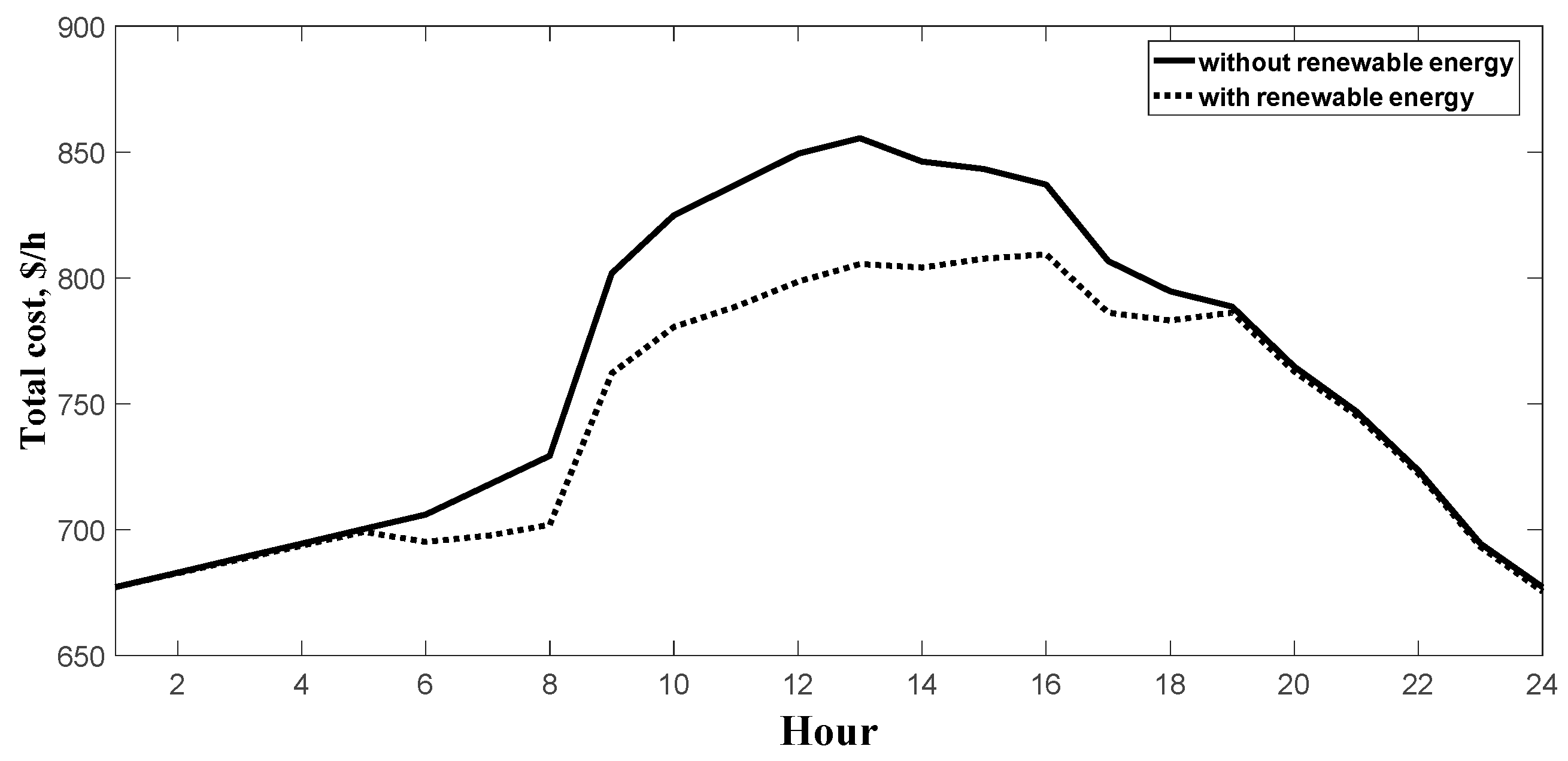
3.2. Total Generation Cost
The cost of the total generation for the cases of conventional generation with and without adoption of renewable energy is shown in Figure 6. During the first and last day hours, the difference in the cost of the two cases is low due to the absence of PV output which makes a limited contribution from renewable energy during these periods.
It can be observed that the cost of generated power is decreased significantly when renewable energy is integrated into the system. Before integration of renewable energy distribution generators, the optimal cost at highest load was 855.4 $/h. However, when renewable energy was integrated, the maximum cost decreased to 809.4 $/h (a 5.4% reduction in cost) under the same conditions. In addition, the occurrence of the maximum cost shifted from hour 13 to hour 16. This has the advantage of shifting the maximum generation cost to low energy cost periods in the case a load management strategy is applied. Moreover, the cost increase trend with load changed from a quadratic form (which is the case of conventional generation cost) to a piecewise linear curve. This means that, the rate of incremental fuel cost is reduced. It was concluded from Figure 6 that the cost of power generation is decreased significantly when renewable energy is integrated into the power system.
3.3. Transmission Losses
Figure 7 shows the transmission power losses for both cases with and without renewable energy. The transmission losses are decreased when distributed renewable generation is integrated into the system. The loads that connected to the buses, where the renewable energy power plants are inserted, are supplied by the renewable energy power plants. Therefore, the power coming from the conventional fuel power plants; far away from these buses; is decreased. Consequently, the power flow in the corresponding transmission lines was low and the transmission lines losses were reduced. If the generated power from renewable energy sources is more than the connected loads to the relevant buses, the extra power is transferred to the buses in the neighborhood depending on OPF methodology.
It can be observed that transmission losses decreased from 10.14 MW; when the contribution of renewable energy sources is zero; to 9.15 MW with the adoption of renewable sources.
4. Sensitivity Analysis
This section is studying effect of some parameters on the power system performance. Since the renewable energy resources are variable and intermittent in nature, the power system performance will definitely be affected. Sensitivity analysis is additionally conducted for considering the error in measurement. Moreover, the load is changing in nature which makes the sensitivity analysis is vital to predict the results with any deviations in the input data.
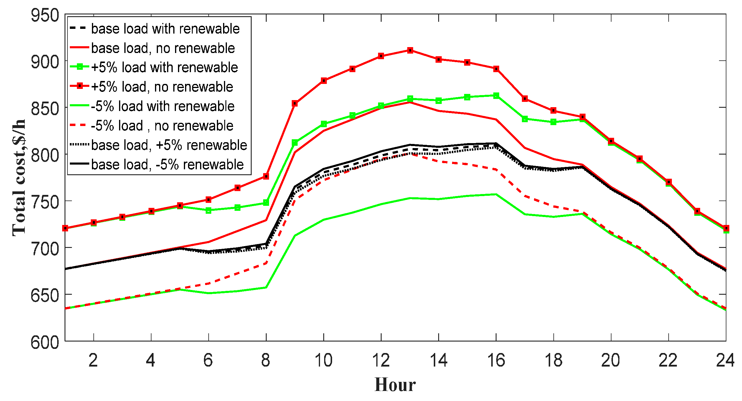
4.1. Effect of Renewable Energy and Load Changes on Generation Cost
The effect of change in renewable energy and change in load demand on total generation cost is shown in Figure 8. A small change of ±5% in both renewable energy generation and load was assumed. This figure shows that the worst case occurs when the load is increased by 5% and the renewable energy contribution is zero. The total cost reached more than 900 $/h. On the other hand, the lowest cost was achieved when there is a renewable energy contribution while the load is decreased by 5%, the total cost becomes 730 $/h.
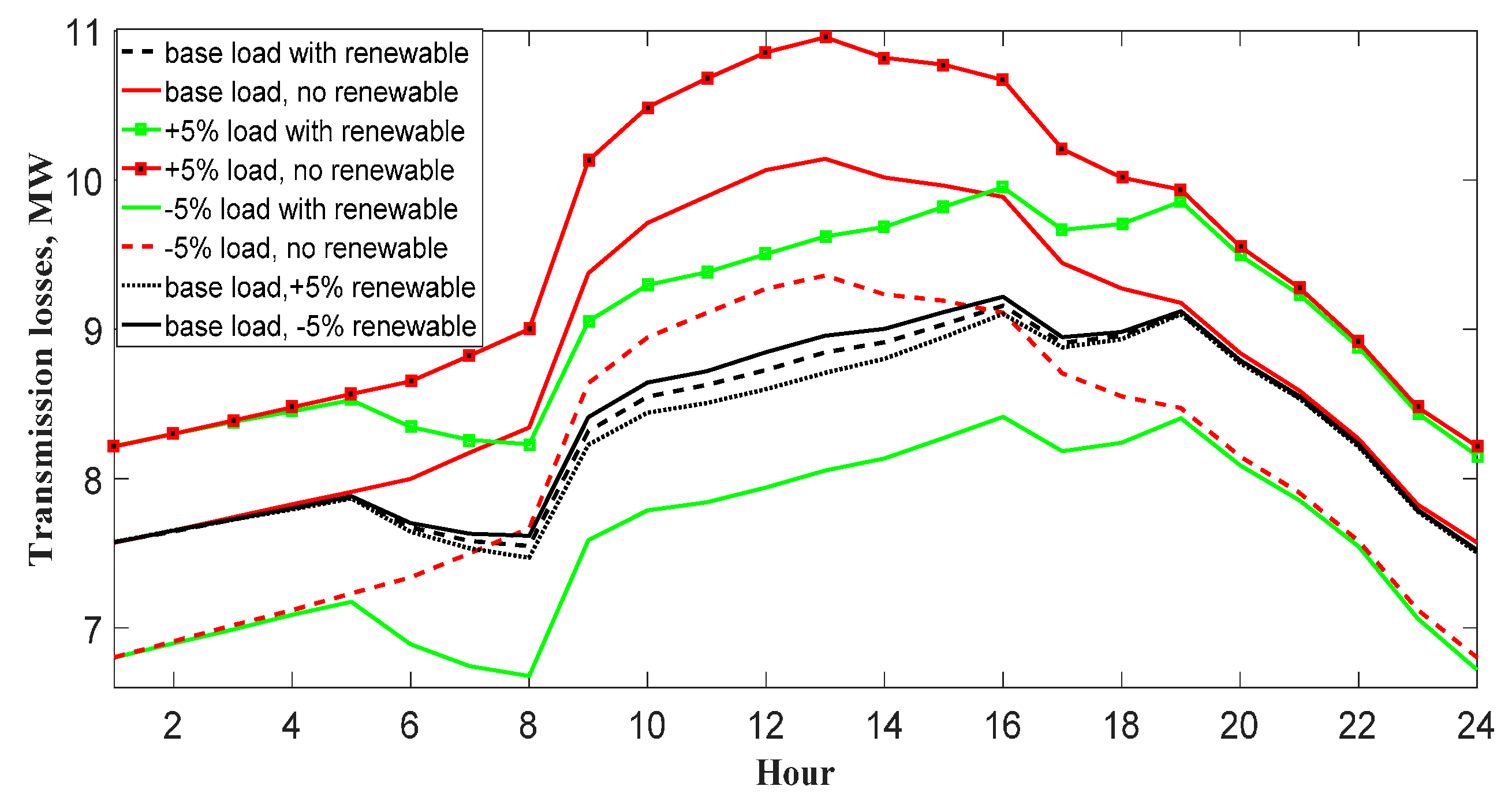
4.2. Effect of Renewable Energy and Load Changes on Transmission Losses
Figure 9 shows the effect of renewable energy capacity variation and the effect of load change on transmission losses of the power system. The load and renewable energy generation are assumed to be changed in the range of ±5%. The solid curve with square marker represents the base case of base load without renewable energy generation contribution and the maximum losses exceeded 10 MW at hour 13. It’s obvious that, the load change has a greater effect than the renewable energy generation change. When load is increased by 5% without using renewable energy sources, the transmission losses reached up to 11 MW, so with a 5% increase in load, one has a 10% increase in transmission line losses in the case the renewable energy sources are not adoped. However, when the load decreased by 5% with zero renewable energy contribution; the transmission losses were less than 9.36 MW. The integration of renewable energy sources reduced these losses to 9.95 MW when the load is increased by 5% (instead of 11 MW), so with a 5% increase in load, there will be more than a 10% reduction in transmission line losses in the case of adoption of the renewable energy sources. Also, the transmission line losses became 8.4 MW when the load is decreased by 5% instead of 9.36 MW, so there is about a 16% reduction in transmission line losses when the load is reduced by 5% when adopting the renewable energy sources. Furthermore, the integration of renewable energy generation transferred the peak value of these losses from hour 13 to hour 16. Therefore, the probability of transmission lines to be congested is shifted from the time when the conventional peak load occurs.
4.3. Effect of Changing Solar PV Efficiency on Total Cost
The efficiency of PV system has a great influence on the total cost of the PV system. The efficiency of PV system used in all above calculations was 15%. The sanctity analysis of PV system efficiency has been carried out by varying its value to 10%, 15% and 20% as shown in Figure 10. It is clear from this figure that the lowering the PV efficiency will increase the cost during the hours having PV contributions and vice versa. During the hours that don't have PV generation contribution the total cost will not change.
4.4. Effect of Changing Coefficient of Performance on Total Cost
As has been shown above for the sensitivity analysis on changing the PV system efficiency, the same study for changing the coefficient of performance of wind energy system has been performed. Three different values, 40%, 45% and 50%, have been used in this study. Due to the limited contribution the effect of changing the coefficient of performance on the cost does not show a considerable influence on the total cost of the power system as seen in Figure 11. It is clear from this figure that the cost is reduced by 1–2% when the coefficient of performance increases from 45% to 50%. The cost also increased by almost the same percentage upon reducing the coefficient of performance from 45% to 50%.
5. Conclusions
The integration of renewable energy in existing power systems in the form of DG was addressed in this study. A 30-bus IEEE power system was used as a case study to assess the advantages and disadvantages of integration of different renewable energy sources in the form of DG. Wind energy and solar energy were integrated into the proposed power system. The results showed an enhancement in the economical operation of fossil fuel generators. The total cost of operation was decreased from 855.4 $/h to 809.4 $/h during peak load periods. The total transmission losses were decreased by 10% in case of renewable energy source use at the selected buses. A sensitivity analysis was performed to investigate the performance of the system under varying uncertain data conditions. In this analysis, the effect of changing the loads by ±5% with and without renewable energy sources on the cost and transmission losses have been examined. The results from the sensitivity analysis show a 5.4% reduction in cost, 16% reduction in transmission line losses in the case of renewable energy source adoption, and a 5% reduction in load compared with the case of no renewable energy source adoption, which prove the superiority of the proposed analysis.
Acknowledgments
The authors extend their appreciation to the International Scientific Partnership Program (ISPP) at King Saud University for funding this research work through ISPP#0047.
Author Contributions
All the authors contributed to the realization, analysis the data of as well as the writing of the paper.
Conflicts of Interest
The authors declare no conflict of interest.
References
- Huneault, M.; Galiana, F.; Bruno, Q. A survey of the optimal power flow literature. IEEE Trans. Power Syst. 1991, 6, 18. [Google Scholar] [CrossRef]
- Zehar, K.; Samir, S. Optimal power flow with environmental constraint using a fast successive linear programming algorithm: Application to the Algerian power system. Energy Convers. Manag. 2008, 49, 3362–3366. [Google Scholar] [CrossRef]
- Shahidehpour, M.; Ramesh, V. Nonlinear Programming Algorithms and Decomposition Strategies for OPF. In IEEE/PES Tutorial on Optimal Power Flow; IEEE: New York, NY, USA, 1996. [Google Scholar]
- Lipowski, J.; Charalambous, C. Solution of optimal load flow problem by modified recursive quadratic-programming method. IEE Proc. Gener. Trans. Distrib. 1981, 5, 288–294. [Google Scholar] [CrossRef]
- Capitanescu, F.; Glavic, M.; Ernst, D.; Wehenkel, L. Interior-point based algorithms for the solution of optimal power flow problems. Electr. Power Syst. Res. 2007, 77, 508–517. [Google Scholar] [CrossRef]
- Sun, D.I.; Ashley, B.; Brewer, B.; Hughes, A.; Tinney, W.F. Optimal power flow by Newton approach. IEEE Trans. Power Appar. Syst. 1984, PAS-103, 2864–2880. [Google Scholar] [CrossRef]
- Bakirtzis, A.G.; Biskas, P.N.; Zoumas, C.E.; Petridis, V. Optimal power flow by enhanced genetic algorithm. IEEE Trans. Power Syst. 2002, 17, 229–236. [Google Scholar] [CrossRef]
- Devaraj, D.; Yegnanarayana, B. Genetic-algorithm-based optimal power flow for security enhancement. IEEE Proc. Gener. Trans. Distrib. 2005, 152, 899–905. [Google Scholar] [CrossRef]
- Sood, Y.R. Evolutionary programming based optimal power flow and its validation for deregulated power system analysis. Int. J. Electr. Power Energy Syst. 2007, 29, 65–75. [Google Scholar] [CrossRef]
- Abido, M. Optimal power flow using particle swarm optimization. Int. J. Electr. Power Energy Syst. 2002, 24, 563–571. [Google Scholar] [CrossRef]
- Mo, N.; Zou, Z.; Chan, K.; Pong, T. Transient stability constrained optimal power flow using particle swarm optimization. IET Gener. Trans. Distrib. 2007, 1, 476–483. [Google Scholar] [CrossRef]
- Jeon, Y.J.; Kim, J.C. Application of simulated annealing and tabu search for loss minimization in distribution systems. Int. J. Electr. Power Energy Syst. 2004, 26, 9–18. [Google Scholar] [CrossRef]
- El Ela, A.A.; Abido, M.; Spea, S. Optimal power flow using differential evolution algorithm. Electr. Power Syst. Res. 2010, 80, 878–885. [Google Scholar] [CrossRef]
- Niknam, T.; Narimani, M.; Jabbari, M.; Malekpour, A.R. A modified shuffle frog leaping algorithm for multi-objective optimal power flow. Energy 2011, 36, 6420–6432. [Google Scholar] [CrossRef]
- Frank, S.; Steponavice, I.; Rebennack, S. Optimal power flow: A bibliographic survey I. Energy Syst. 2012, 3, 221–258. [Google Scholar] [CrossRef]
- Roy, P.; Chakrabarti, A. Modified shuffled frog leaping algorithm with genetic algorithm crossover for solving economic load dispatch problem with valve-point effect. Appl. Soft Comput. 2013, 13, 4244–4252. [Google Scholar] [CrossRef]
- Liu, S.; Hou, Z.; Wang, M. A Hybrid Algorithm for Optimal Power Flow Using the Chaos Optimization and the Linear Interior Point Algorithm. In Proceedings of the PowerCon 2002 International Conference on Power System Technology, Kunming, China, 13–17 October 2002; pp. 793–797. [Google Scholar]
- Saini, A.; Chaturvedi, D.K.; Saxena, A. Optimal power flow solution: A GA-fuzzy system approach. Int. J. Electr. Power Energy Syst. 2006, 5. [Google Scholar] [CrossRef]
- Kumar, S.; Chaturvedi, D. Optimal power flow solution using fuzzy evolutionary and swarm optimization. Int. J. Electr. Power Energy Syst. 2013, 47, 416–423. [Google Scholar] [CrossRef]
- Rajaram, R.; Kumar, K.S.; Rajasekar, N. Power system reconfiguration in a radial distribution network for reducing losses and to improve voltage profile using modified plant growth simulation algorithm with Distributed Generation (DG). Energy Rep. 2015, 1, 116–122. [Google Scholar] [CrossRef]
- Arya, L.; Koshti, A.; Choube, S. Distributed generation planning using differential evolution accounting voltage stability consideration. Int. J. Electr. Power Energy Syst. 2012, 42, 196–207. [Google Scholar] [CrossRef]
- Guerriche, K.R.; Bouktir, T. Optimal allocation and sizing of distributed generation with particle swarm optimization algorithm for loss reduction. Rev. Sci. Technol. 2015, 6, 59–69. [Google Scholar]
- Rao, R.S.; Ravindra, K.; Satish, K.; Narasimham, S. Power loss minimization in distribution system using network reconfiguration in the presence of distributed generation. IEEE Trans. Power Syst. 2013, 28, 317–325. [Google Scholar] [CrossRef]
- Kowsalya, M. Optimal size and siting of multiple distributed generators in distribution system using bacterial foraging optimization. Swarm Evol. Comput. 2014, 15, 58–65. [Google Scholar]
- Eltamaly, A.; Mohamed, M.; Abdulrahman, A. A novel smart grid theory for optimal sizing of hybrid renewable energy systems. Sol. Energy 2016, 124, 26–38. [Google Scholar] [CrossRef]
- Eltamaly, A.; Addoweesh, K.; Bawa, U.; Mohamed, A. Economic modeling of hybrid renewable energy system: A case study in Saudi Arabia. Arab. J. Sci. Eng. 2014, 39, 3827–3839. [Google Scholar] [CrossRef]
- Mohamed, A.; Eltamaly, A.; Alolah, I. Swarm intelligence-based optimization of grid-dependent hybrid renewable energy systems. Renew. Sustain. Energy Rev. 2017, 77, 515–524. [Google Scholar] [CrossRef]
- Eltamaly, A.; Mohamed, A. A novel design and optimization software for autonomous PV/wind/battery hybrid power systems. Math. Probl. Eng. 2014, 2014, 637174. [Google Scholar] [CrossRef]
- Mohamed, A.; Eltamaly, A.; Alolah, I. Sizing and techno-economic analysis of stand-alone hybrid photovoltaic/wind/diesel/battery power generation systems. J. Renew. Sustain. Energy 2015, 7, 063128. [Google Scholar] [CrossRef]
- Žilinskas, A.; Zhigljavsky, A. Stochastic global optimization: A review on the occasion of 25 Years of informatica. Informatica 2016, 27, 229–256. [Google Scholar] [CrossRef]
- Žilinskas, A.; Žilinskas, J. A hybrid global optimization algorithm for non-linear least squares regression. J. Glob. Optim. 2013, 56, 265–277. [Google Scholar] [CrossRef]
- Kennedy, J.; Kennedy, F.; Eberhart, C.; Shi, Y. Swarm Intelligence; Morgan Kaufmann Publishers Inc.: San Francisco, CA, USA, 2001. [Google Scholar]
- Settles, M. An Introduction to Particle Swarm Optimization; Department of Computer Science, University of Idaho: Moscow, ID, USA, 2005; pp. 1–8. [Google Scholar]
- Elbeltagi, E.; Hegazy, T.; Grierson, D. Comparison among five evolutionary-based optimization algorithms. Adv. Eng. Inf. 2005, 19, 43–53. [Google Scholar] [CrossRef]
- Qiu, Z.; Deconinck, G.; Belmans, R. A Literature Survey of Optimal Power Flow Problems in the Electricity Market Context. In Proceedings of the 2009 PSCE ’09 IEEE/PES Power Systems Conference and Exposition, Seattle, WA, USA, 15–18 March 2009; pp. 1845–1850. [Google Scholar]
- Soliman, S.; Mantawy, A. Modern Optimization Techniques with Applications in Electric Power Systems; Springer Science & Business Media: Berlin, Germany, 2011. [Google Scholar]
- Wagner, F. Renewables in Future Power Systems; Springer: Berlin, Germany, 2014. [Google Scholar]
- Jarass, L.; Obermair, G.M.; Voigt, W. Windenergie: Zuverlässige Integration in die Energieversorgung; Springer-Verlag: Berlin, Germany, 2009. [Google Scholar]
- 30-Bus Power Flow Test Case. Available online: https://www2.ee.washington.edu/research/pstca/pf30/pg_tca30bus.htm (accessed on 17 July 2017).
- Asano, H.; Yajima, K.; Kaya, Y. Influence of photovoltaic power generation on required capacity for load frequency control. IEEE Trans. Energy Convers. 1996, 11, 188–193. [Google Scholar] [CrossRef]
- Bebic, J. Power System Planning: Emerging Practices Suitable for Evaluating the Impact of High-Penetration Photovoltaics; National Renewable Energy Laboratory: Golden, CO, USA, 2008. [Google Scholar]
- Doyle, C.; Loomans, L.; Truitt, A.; Lockhart, R.; Golden, M.; Dabbagh, K.; Lawrence, R. Solar Access to Public Capital (SAPC) Working Group: Best Practices in Commercial and Industrial (C&I) Solar Photovoltaic System Installation; Period of Performance. November 28, 2014–September 1, 2015; NREL (National Renewable Energy Laboratory (NREL): Golden, CO, USA, 2015. [Google Scholar]
- Masebinu, S.; Akinlabi, E.; Muzenda, E.; Aboyade, A. Renewable Energy: Deployment and the Roles of Energy Storage. In Proceedings of the World Congress on Engineering, London, UK, 29 June–1 July 2016. [Google Scholar]
Figure 1.
Single line diagram of 30-bus IEEE case test.

Figure 2.
Buses’ voltage magnitude with and without renewable energy generation.

Figure 3.
Total system load over 24 h.

Figure 4.
Solar, wind and total renewable power generation.

Figure 5.
Total conventional energy generation with and without renewable energy generation.

Figure 6.
Total cost of generation with and without renewable energy.

Figure 7.
Total transmission losses with and without renewable energy, MW.

Figure 8.
Cost of total generation of the system including renewable energy generation.

Figure 9.
Effect of change in renewable energy and load in transmission losses.

Figure 10.
Effect of changing solar PV efficiency on total cost.

Figure 11.
Effect of changing coefficient of performance on total cost.


Table 1.
Comparison of different methods to 30-bus power system model. GA: genetic algorithm; RGA: real genetic algorithm; OPF: optimal power flow.
Table 1.
Comparison of different methods to 30-bus power system model. GA: genetic algorithm; RGA: real genetic algorithm; OPF: optimal power flow.
| Method | Project Gradient | Tabu Search | GA | RGA | GA OPF | GAF OPF | Proposed Model |
|---|---|---|---|---|---|---|---|
| Total cost ($/h) | 813.74 | 802.29 | 805.94 | 804.02 | 802.38 | 802.0003 | 801.8 |
© 2017 by the authors. Licensee MDPI, Basel, Switzerland. This article is an open access article distributed under the terms and conditions of the Creative Commons Attribution (CC BY) license (http://creativecommons.org/licenses/by/4.0/).
Share and Cite
MDPI and ACS Style
Khaled, U.; Eltamaly, A.M.; Beroual, A. Optimal Power Flow Using Particle Swarm Optimization of Renewable Hybrid Distributed Generation. Energies 2017, 10, 1013. https://doi.org/10.3390/en10071013
AMA Style
Khaled U, Eltamaly AM, Beroual A. Optimal Power Flow Using Particle Swarm Optimization of Renewable Hybrid Distributed Generation. Energies. 2017; 10(7):1013. https://doi.org/10.3390/en10071013
Chicago/Turabian StyleKhaled, Usama, Ali M. Eltamaly, and Abderrahmane Beroual. 2017. "Optimal Power Flow Using Particle Swarm Optimization of Renewable Hybrid Distributed Generation" Energies 10, no. 7: 1013. https://doi.org/10.3390/en10071013
Note that from the first issue of 2016, this journal uses article numbers instead of page numbers. See further details here.