
Strategic Maintenance Scheduling of an Offshore Wind Farm in a Deregulated Power System


Abstract
:1. Introduction
2. Problem Formulation
2.1. Cost-Minimization Maintenance Scheduling
2.2. Profit-Maximization Maintenance Scheduling
2.3. Karush–Kuhn–Tucker Conditions
3. Case Study
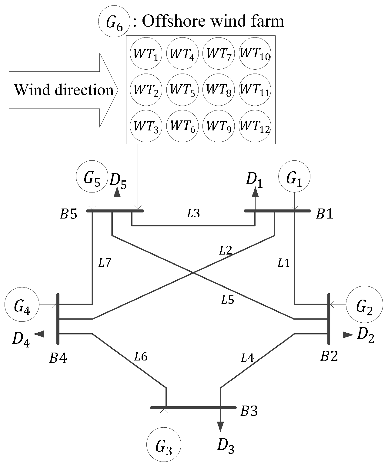
3.1. Test System
3.2. Cases
3.2.1. Case I
3.2.2. Case II
3.2.3. Case III
3.2.4. Case IV
3.2.5. Case V
3.2.6. Case VI
3.2.7. Case VII
3.2.8. Case VIII
3.2.9. Case IX
4. Results
5. Conclusions
Acknowledgments
Author Contributions
Conflicts of Interest
Nomenclature
| Indices: | |
| Index for bus | |
| h | Index for hour |
| k | Index for wind turbine |
| g | Index for generation unit |
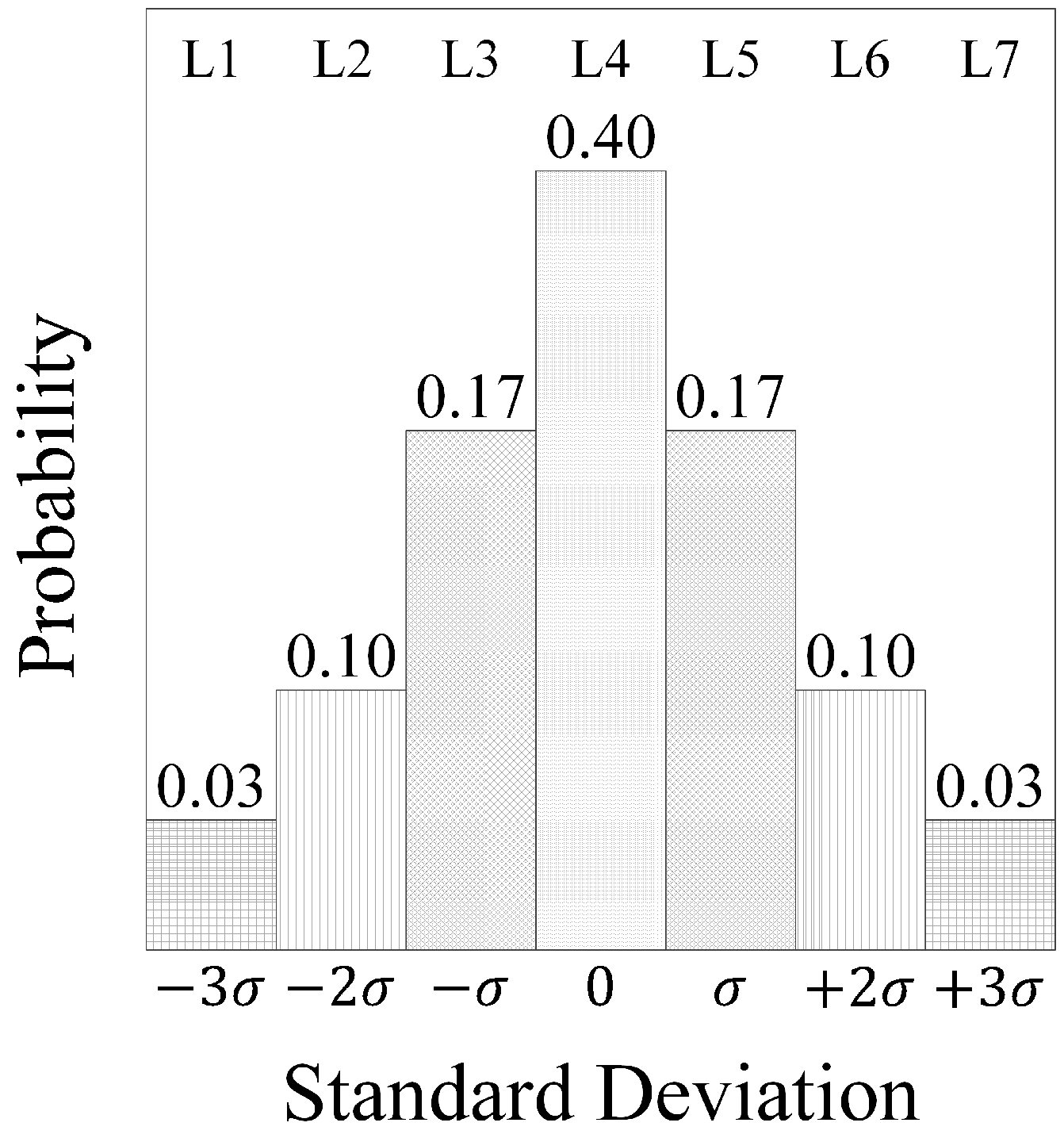
| s | Index for stochastic scenario |
| r | Index for maintenance round (number) |
| Sets: | |
| Buses connected to bus i | |
| Generators connected to bus i | |
| Parameters: | |
| Incremental term of fuel consumption (MBTU/MW) of generator g | |
| Cost of fuel ($/MBTU) of generator g | |
| Variable operation cost ($/MW) of generator g | |
| Maximum capacity (MW) of generator at time h | |
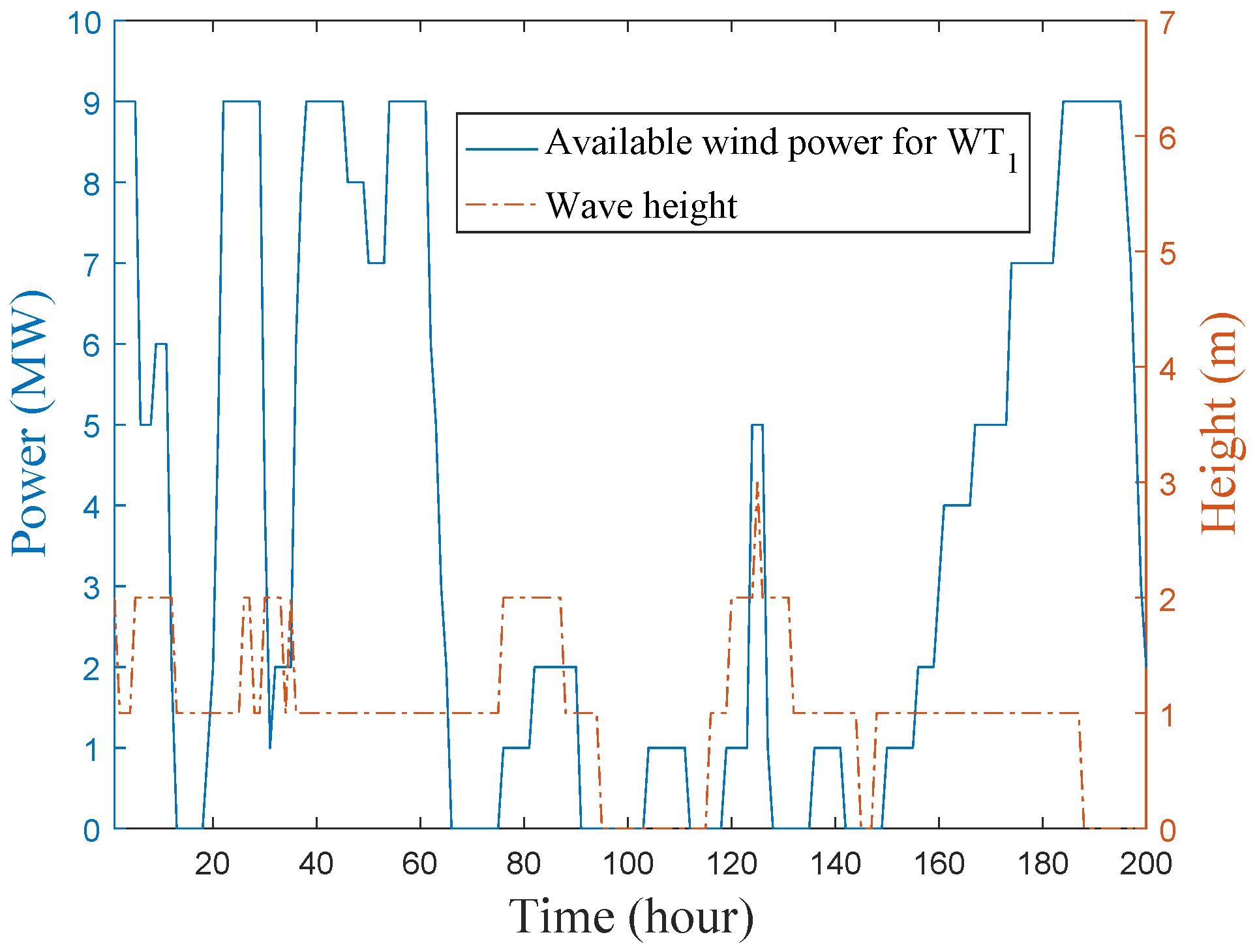
| Maximum available wind power (MW) of wind turbine k at time h and scenario s in | |
| Inductance (Ω) of line between buses i and j | |
| Capacity (MW) of line between buses i and j | |
| Demand (MW) at hour h and bus i | |
| Maintenance action duration for each wind turbine k at OWF | |
| Maintenance action duration for | |
| C | Maintenance action cost ($) |
| Z | Maximum simultaneous maintenance actions |
| τ | Night time parameter |
| Cost factor for vessel b | |
| Wave height prediction (m) at hour h and scenario s | |
| Wave height limit (m) for vessel b | |
| Transportation time (hour) for vessel b between wind turbine k and shore | |
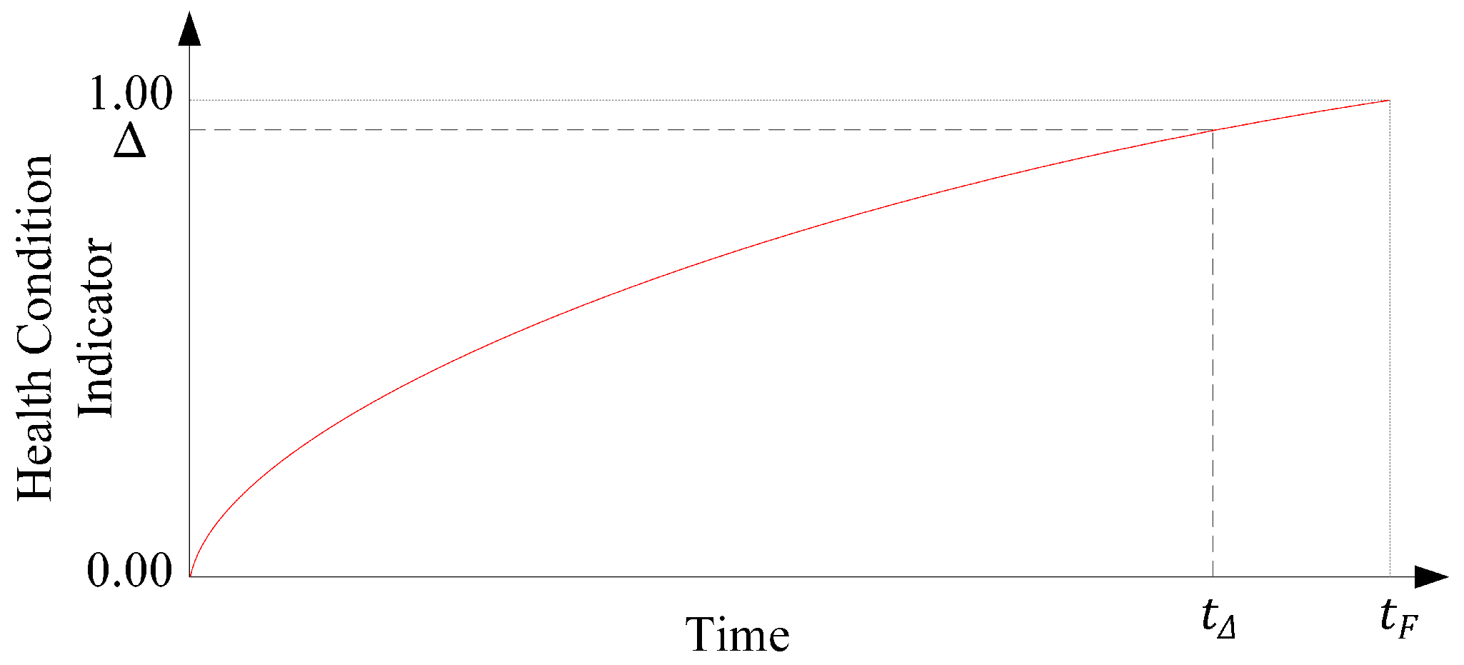
| Maximum time limit for maintenance from alarm signal of condition monitoring system | |
| Wind turbine that has received an alarm signal | |
| Number of time periods | |
| Number of generators | |
| Number of buses | |
| Number of stochastic scenarios | |
| Number of maintenance rounds | |
| Sufficiently large numbers | |
| Variables: | |
| Power generation (MW) of unit g at hour h and scenario s | |
| Voltage angle (rad) in node i at hour h and scenario s | |
| Binary variable of maintenance status of WT k at hour h with vessel b on maintenance action r | |
| Binary variable of utilization status of vessel b for WT k at hour h on maintenance action r | |
| Binary variable of maintenance status of generator g (except OWF) at hour h on maintenance action r | |
| Electricity price at hour h, bus i and scenario s | |
| Lagrange multiplier of demand balance | |
| Lagrange multiplier of power-flow | |
| Lagrange multiplier of maximum capacity limit for | |
| Lagrange multiplier of maximum capacity limit for | |
| Lagrange multiplier of capacity positivity | |
| Variable used for linearization in strong duality | |
| Variable used for linearization in strong duality | |
References
- Castro-Santos, L.; Diaz-Casas, V. Resource Assessment Methods in the Offshore Wind Energy Sector. In Floating Offshore Wind Farms; Springer: Basel, Switzerland, 2016; pp. 121–141. [Google Scholar]
- Musial, W.; Ram, B. Large-Scale Offshore Wind Power in the United States, Assessment of Opportunities and Barriers; Offshore Wind Hub: Cambridge, MA, USA, 2010; p. 221. [Google Scholar]
- Maples, B.; Saur, G.; Hand, M.; van de Pietermen, R.; Obdam, T. Installation, Operation, and Maintenance Strategies to Reduce the Cost of Offshore Wind Energy; Offshore Wind Hub: Cambridge, MA, USA, 2013; p. 89. [Google Scholar]
- Tavner, P. Overview of Offshore Wind Development. In Offshore Wind Turbines: Reliability, Availability & Maintenance; The Institution of Engineering and Technology IET: Stevenage, UK, 2012; p. 296. [Google Scholar]
- Van Bussel, G.; Henderson, A.; Morgan, C.; Smith, B.; Barthelmie, R.; Argyriadis, K.; Arena, A.; Niklasson, G.; Peltola, E. State of the Art and Technology Trends for Offshore Wind Energy: Operation and Maintenance Issues. In Proceedings of the Offshore Wind Energy EWEA Special Topic Conference, Brussels, Belgium, 10–12 December 2001.
- Tavner, P. Maintenance for Offshore Wind Turbines. In Offshore Wind Turbines: Reliability, Availability & Maintenance; IET: Stevenage, UK, 2012; p. 296. [Google Scholar]
- El-Thalji, I.; Liyanage, J.P. On the Operation and Maintenance Practices of Wind Power Asset: A status review and observations. J. Qual. Maint. Eng. 2012, 18, 232–266. [Google Scholar] [CrossRef]
- Dawid, R.; mcMillan, D.; Revie, M. Review of Markov Models for Maintenance Optimization in the Context of Offshore Wind. In Proceedings of the Annual Conference of the Prognostics and Health Management Society, Coronado, CA, USA, 18–24 October 2015; PHM Society: Coronado, CA, USA, 2015; Volume 6. [Google Scholar]
- Abdollahzadeh, H.; Atashgar, K.; Abbasi, M. Multi-Objective Opportunistic Maintenance Optimization of a Wind Farm considering Limited Number of Maintenance Groups. Renew. Energy 2016, 88, 247–261. [Google Scholar] [CrossRef]
- Sarker, B.R.; Faiz, T.I. Minimizing Maintenance Cost for Offshore Wind Turbines following Multi-level Opportunistic Preventive Strategy. Renew. Energy 2015, 85, 104–113. [Google Scholar] [CrossRef]
- Shafiee, M.; Finkelsteinb, M.; Berenguer, C. An Opportunistic Condition-based Maintenance Policy for Offshore Wind Turbine Blades Subjected to Degradation and Environmental Shocks. Reliab. Eng. Syst. Saf. 2015, 142, 463–471. [Google Scholar] [CrossRef]
- Mazidi, P.; Du, M.; Bertling, L.T.; Sanz-Bobi, M.A. A Performance and Maintenance Evaluation Framework for Wind Turbines. In Proceedings of the International Conference on Probabilistic Methods Applied to Power Systems (PMAPS), Beijing, China, 16–20 October 2016.
- Mazidi, P.; Du, M.; Sanz-Bobi, M.A. A Comparative Study of Techniques Utilized in Analysis of Wind Turbine Data. In Proceedings of the China International Conference on Electricity Distribution (CICED), Xi’an, China, 10–12 August 2016.
- Mazidi, P.; Bertling, L.T.; Sanz-Bobi, M.A. Wind Turbine Prognostics and Maintenance Management based on a Hybrid Approach of Neural Networks and Proportional Hazards Model. J. Risk Reliab. 2016. [Google Scholar] [CrossRef]
- Marugan, A.P.; Marquez, F.P.G.; Perez, J.M.P. Optimal Maintenance Management of Offshore Wind Farms. Energies 2016, 9, 46. [Google Scholar] [CrossRef]
- Shafiee, M. Maintenance Logistics Organization for Offshore Wind Energy: Current Progress and Future Perspectives. Renew. Energy 2016, 77, 182–193. [Google Scholar] [CrossRef]
- Dinwoodie, I.; Endrerud, O.E.V.; Hofmann, M.; Martin, R.; Sperstad, I.B. Reference Cases for Verification of Operation and Maintenance Simulation Models for Offshore Wind Farms. Wind Eng. 2015, 39, 1–14. [Google Scholar] [CrossRef]
- Hofmann, M. A Review of Decision Support Models for Offshore Wind Farms with an Emphasis on Operation and Maintenance Strategies. Wind Eng. 2011, 35, 1–16. [Google Scholar] [CrossRef]
- Douard, F.; Domecq, C.; Lair, W. A Probabilistic Approach to Introduce Risk Measurement Indicators to an Offshore Wind Project Evaluation—Improvement to an existing tool. In Proceedings of the 11th International Probabilistic Safety Assessment and Management Conference and the Annual European Safety and Reliability Conference, Helsinki, Finland, 25–29 June 2012; pp. 358–364.
- Scheu, M.; Matha, D.; Hofmann, M.; Muskulus, M. Maintenance Strategies for Large Offshore Wind Farms. In Proceedings of the Energy Procedia: Deep Sea Offshore Wind R&D Conference, Trondheim, Norway, 19–20 January 2012; Volume 24, pp. 281–288.
- Browell, J.; Zitrou, A.; Walls, L.; Bedford, T.; Infield, D. Analysis of Wind and Wave Data to Assess Maintenance Access to Offshore Wind Farms. In Safety, Reliability and Risk Analysis: Beyond the Horizon; CRC Press: Amsterdam, The Netherlands, 2013; pp. 743–750. [Google Scholar]
- Besnard, F.; Patrikssont, M.; Strombergt, A.B.; Wojciechowski, A.; Tjernberg, L.B. An Optimization Framework for Opportunistic Maintenance of Offshore Wind Power System. In Proceedings of the 2009 IEEE Bucharest PowerTech, Bucharest, Romania, 28 June–2 July 2009.
- Besnard, F.; Fischer, K.; Tjernberg, L.B. A Model for the Optimization of the Maintenance Support Organization for Offshore Wind Farms. IEEE Trans. Sustain. Energy 2013, 4, 443–450. [Google Scholar] [CrossRef]
- Dalgic, Y.; Lazakis, I.; Dinwoodie, I.; McMillan, D.; Revie, M. Advanced Logistics Planning for Offshore Wind Farm Operation and Maintenance Activities. Ocean Eng. 2015, 101, 211–226. [Google Scholar] [CrossRef]
- Simani, S. Overview of Modelling and Advanced Control Strategies for Wind Turbine Systems. Energies 2015, 8, 13395–13418. [Google Scholar] [CrossRef]
- Van Bussel, G.; Zaaijer, M. Reliability, Availability and Maintenance Aspects of Large-scale Offshore Wind Farms, a Concepts Study. In Proceedings of the MAREC Marine Renewable Energies Conference, Newcastle, UK, 27–28 March 2001; pp. 119–126.
- Martin, R.; Lazakis, I.; Barbouchi, S.; Johanning, L. Sensitivity Analysis of Offshore Wind Farm Operation and Maintenance Cost and Availability. Renew. Energy 2016, 85, 1226–1236. [Google Scholar] [CrossRef] [Green Version]
- Wang, Y.; Handschin, E. A New Genetic Algorithm for Preventive Unit Maintenance Scheduling of Power Systems. Int. J. Electr. Power Energy Syst. 2000, 22, 343–348. [Google Scholar] [CrossRef]
- Perez-Canto, S.; Rubio-Romero, J.C. A Model for the Preventive Maintenance Scheduling of Power Plants including Wind Farms. Reliab. Eng. Syst. Saf. 2013, 119, 67–75. [Google Scholar] [CrossRef]
- Mazidi, P.; Bobi, M.A.S. Implementation of Risk in Generation Planning. In Proceedings of the 10th Workshop on Industrial Systems and Energy Technologies, Peradeniya, Sri Lanka, 18–20 December 2015.
- Froger, A.; Gendreau, M.; Mendoza, J.E.; Pinson, E.; Rousseau, L.M. Maintenance Scheduling in the Electricity Industry: A Literature Review. Eur. J. Oper. Res. 2016, 251, 695–706. [Google Scholar] [CrossRef]
- Chinneck, J.W. Chapter 20—The Karush-Kuhn-Tucker (KKT) Conditions. In Practical Optimization: A Gentle Introduciton; Carleton University: Ottawa, ON, Canada, 2015. [Google Scholar]
- Fortuny-Amat, J.; McCarl, B. A Representation and Economic Interpretation of a Two-Level Programming Problem. J. Oper. Res. Soc. 1981, 32, 783–792. [Google Scholar] [CrossRef]
- Rosenthal, R.E. GAMS—A User’s Guide; GAMS Development Corporation: Washington, DC, USA, 2016. [Google Scholar]
- User’s Manual for CPLEX; Technical Report; IBM Corp.: Armonk, NY, USA, 2016.
- National Data Buoy Center, National Weather Service Organization. 2017. Available online: http://www.ndbc.noaa.gov/ (accessed on 1 Febuary 2017).
- De Andrade Vieira, R.; Sanz-Bobi, M.A. Failure Risk Indicators for a Maintenance Model Based on Observable Life of Industrial Components With an Application to Wind Turbines. IEEE Trans. Reliab. 2013, 62, 569–582. [Google Scholar] [CrossRef]
- Ribrant, J.; Bertling-Tjernberg, L. Survey of failures in wind power systems with focus on Swedish wind power plants during 1997–2005. In Proceedings of the IEEE Power Engineering Society General Meeting, Tampa, FL, USA, 24–28 June 2007.
- Report on Wind Turbine Subsystem Reliability—A Survey of Various Databases; Technical Report NREL/PR- 5000-59111; National Renewable Energy Laboratory NREL: Golden, CO, USA, 2013.


| Generator | ||||
|---|---|---|---|---|
| G1 | 100 | 0.3 | 5 | 7 |
| G2 | 90 | 0.5 | 10 | 9 |
| G3 | 160 | 0.7 | 15 | 11 |
| G4 | 80 | 0.9 | 20 | 13 |
| G5 | 70 | 1.1 | 25 | 15 |
| G6 | 108 | 0 | 0 | 10 |
| Wind Turbine | Vessel Transfer Time (h) | Wake Effect (MW) | FOR | ||
|---|---|---|---|---|---|
| (Hourly Measure) | (p.u.) | ||||
| 2 | 1 | 0 | Figure 3 | 0.02 | |
| 2 | 1 | 0 | Figure 3; 1 | 0.02 | |
| 2 | 1 | 0 | Figure 3; 2 | 0.01 | |
| 2 | 1 | 0 | Figure 3; 3 | 0.01 | |
| Vessel | Vessel Cost Factor | Wave Height Limit (m) |
|---|---|---|
| 0.1 | 0.5 | |
| 0.2 | 1.5 | |
| 0.8 | - |
| Number of Vessel Utilization | Profit ($) | |||
|---|---|---|---|---|
| Case I | 3 (2) | 9 (10) | 0 (0) | 4716 (9875) |
| Case II | 3 (3) | 9 (9) | 0 (0) | 10,769 (11,410) |
| Case III | 3 (2) | 9 (7) | 0 (3) | 5220 (10,423) |
| Case IV | 3 (2) | 9 (10) | 0 (0) | 10,483 (10,632) |
| Case V | 2 (2) | 10 (10) | 0 (0) | 9810 (10,607) |
| Case VI | 3 (2) | 9 (10) | 0 (0) | 28,204 (25,489) |
| Case VII | 4 (4) | 8 (8) | 0 (0) | 10,867 (17,104) |
| Case VIII | 3 (-) | 9 (-) | 0 (-) | 3498 (-) |
| Case IX | 6 (-) | 18 (-) | 0 (-) | 14,954 (-) |
| Avg.Price ($/MWh) | Operation Cost ($) | |
|---|---|---|
| Case I | 23.310 (23.112) | 929,069 (923,347) |
| Case II | 23.722 (23.211) | 930,450 (924,639) |
| Case III | 23.373 (23.855) | 929,221 (924,250) |
| Case IV | 23.681 (23.755) | 930,299 (924,687) |
| Case V | 23.688 (24.090) | 930,471 (923,995) |
| Case VI | 22.948 (22.357) | 908,732 (900,718) |
| Case VII | 23.675 (23.892) | 930,222 (925,036) |
| Case VIII | 23.363 (-) | 930,855 (-) |
| Case IX | 25.855 (-) | 919,536 (-) |
| 3 (1) | 4 (6) | 0 (0) | |
| 0 (1) | 7 (6) | 0 (0) | |
| 3 (2) | 4 (4) | 0 (1) | |
| 5 (2) | 2 (5) | 0 (0) | |
| 2 (1) | 5 (5) | 0 (1) | |
| 1 (1) | 6 (5) | 0 (1) | |
| 3 (4) | 4 (3) | 0 (0) | |
| 0 (1) | 7 (6) | 0 (0) | |
| 1 (1) | 6 (6) | 0 (0) | |
| 1 (1) | 6 (6) | 0 (0) | |
| 1 (1) | 6 (6) | 0 (0) | |
| 1 (1) | 6 (6) | 0 (0) |
© 2017 by the authors. Licensee MDPI, Basel, Switzerland. This article is an open access article distributed under the terms and conditions of the Creative Commons Attribution (CC BY) license ( http://creativecommons.org/licenses/by/4.0/).
Share and Cite
Mazidi, P.; Tohidi, Y.; Sanz-Bobi, M.A. Strategic Maintenance Scheduling of an Offshore Wind Farm in a Deregulated Power System. Energies 2017, 10, 313. https://doi.org/10.3390/en10030313
Mazidi P, Tohidi Y, Sanz-Bobi MA. Strategic Maintenance Scheduling of an Offshore Wind Farm in a Deregulated Power System. Energies. 2017; 10(3):313. https://doi.org/10.3390/en10030313
Chicago/Turabian StyleMazidi, Peyman, Yaser Tohidi, and Miguel A. Sanz-Bobi. 2017. "Strategic Maintenance Scheduling of an Offshore Wind Farm in a Deregulated Power System" Energies 10, no. 3: 313. https://doi.org/10.3390/en10030313