1. Introduction
Electricity generation presents many issues and is studied with different techniques in order to reduce its production cost and environmental impact. Conventional production with fossil fuels presents problems associated with the high cost, rapid depletion and detrimental environmental effects of these fuels. Renewable energy is probably the best solution for environmental issues, and many solutions have been developed since the last century, such as hydropower, hydrogen, fuel cells, biofuels, and solar power generation.
Among the renewable sources, small hydropower represents a very attractive source of energy generation. In many countries, small and micro hydropower systems are an important means of electricity generation. An efficient solution, from the point of view of energy efficiency, is the adoption of a turbine, but the purchase and maintenance costs of turbines make their implementation economically unattractive, especially for small hydropower [
1,
2,
3,
4,
5,
6].
Reverse-running centrifugal pumps (also called pumps as turbines or PAT) are a solution for generating and recovering power in small and micro hydropower situations. Pumps are relatively simple machines, inexpensive (compared to a hydraulic turbines), and readily available worldwide. It has been estimated that the capital payback period of a reverse-running pump in the range of 5–50 kW is less than two years [
7,
8]. Moreover, the use of PAT could be suitable because manufacturers of turbines worldwide are less numerous than pump producers, the market for turbines is smaller compared to pumps, and pumps are mechanically simple and require less maintenance. Moreover, an integral pump and electric motor can be purchased for use as a turbine and generator set; pumps are available in a wide range of heads and flows and in a large number of standard sizes. Generally, pumps have short delivery times, spare parts (such as seals and bearings) are easily available and the installation can be done using standard pipes and fittings.
The use of a pump running in reverse mode to generate electricity is not new; the first applications started almost 80 or 90 years ago and many theoretical and experimental studies have been done [
2,
3,
4,
5,
6,
9,
10]. Much research is still being conducted, especially to predict the operating conditions and the efficiency of centrifugal pumps running in reverse [
11].
The selection of a proper PAT for an existing site represents a critical issue because pump manufacturers do not supply the characteristic of the pump running in reverse. Many methods have been used to predict the inverse characteristic of a pump, based on numerical models, experiments, or theoretical procedures [
4,
5,
6,
7,
8,
9,
10].
This research has demonstrated that these methods can be used only for a limited set of pumps. None of them, in fact, allows prediction for the reverse running conditions for all geometries and over a wide range of pump specific speeds. Several studies, based on a modeling approach with CFD code, are available and generally show good correspondence with the available experimental data [
4,
10].
A study [
4] carried out with a computational model of a PAT is based on the concept called “flow zone”. The flow regime within a PAT is divided into four major flow regions (volute casing, impeller, casing outlet and draft tube). A comparison has been made between the experimental and numerical results of a single stage end suction centrifugal pump that was operated in turbine mode at a speed of 800 rpm. CFD predictions of the hydraulic parameters were in good correspondence with the experimental results, but deviations (within 5% to 10%) have been found at certain load regions.
Nautiyal et al. [
5,
6] carried out a study on the application of CFD and its limitations for PAT using cases reported by previous researchers [
4,
9,
10]. The study reported that CFD analysis was an effective design tool for predicting the performance of centrifugal pumps in turbine mode and for identifying the losses in turbo-machinery components such as the draft tube, impeller and casing, but there was some deviation between the experimental results and the CFD modeling results. Barrio et al. [
11] carried out a numerical investigation on the unsteady flow in commercial centrifugal pumps operating in direct and reverse mode with the help of CFD code. The results of their simulation were in good correspondence with the experimental results. The study revealed that in the reverse mode, the flow only matched the geometry of the impeller at nominal conditions; re-circulating fluid regions developed at low flow rates (near the discharge side of the blades) and high flow rates (near the suction side).
Many correlations based on theoretical approaches are available to predict the performance of a PAT. Several researchers (Stepanoff, Childs, Sharma, Wong, Williams, Alatorre-Frenk, and others) have presented correlations for predicting the performance of a pump-as-turbine [
5]. These correlations were based upon either pump efficiency or specific speed. However, deviations of more than 20% have been found between the experimental and predicted reverse operation of standard pumps [
12]. The objective of these correlations is to calculate the best efficiency point (BEP) of pumps for operation in turbine mode by using the pump operation data provided by the manufacturer.
In 1962, Childs [
13] presented a PAT prediction method based on the efficiency of the pump. A similar approach was then presented by McClaskey and Lundquist [
14] and Lueneburg and Nelson [
15] in 1976 and 1985, respectively.
Hancock [
16] stated that for most pumps the turbine BEP lies within 2% of the pump mode BEP. Grover and Hergt [
17,
18] proposed a PAT prediction method based on specific speed for the turbine mode (obtained similar to the specific speed for a pump). Grover’s method is applicable for the turbine mode specific speed range between 10 and 50 [
17]. A comparison between experimental results and the methods proposed by the above researchers show relatively large deviations; therefore, the use of these formulae must be confined to an approximate selection of PATs.
Finally, a large number of experimental studies can be used to evaluate the inverse characteristics. These are often limited to the specific pumps tested, so that they cannot serve as a valid tool for pump selection, but are very useful for tuning and validating theoretical and modeling analyses.
In this paper, authors present a methodology for obtaining the reverse characteristics of a pump, starting from the results of three-dimensional CFD models. After a description of all prediction methods available in the literature, in the third section the adopted modeling approach is described. Three pumps have been studied and modeled using the three-dimensional CFD commercial code PumpLinx®, developed by Simerics Inc.® (1750 112th Ave NE, Ste C250, Bellevue, WA, USA). In the fourth section, the test bench layout is shown with all the transducers’ characteristics.
Numerical models have been validated with experimental data obtained on a dedicated test bench installed in the Department of Civil Construction and Environmental Engineering of the University of Naples Federico II. Simulations have been run in both direct (as pump) and reverse (as turbine) modes with good accuracy.
In the fifth section, the models’ results have been used to predict the efficiency curves of the three analyzed pumps in both modes. At the end of the paper, results of the proposed methodology have been compared to the prediction methods described in the second section. Analysis has demonstrated that the existing prediction methods underestimate or overestimate the real operation.
In this paper, the authors have shown only the first step of a research done on PAT. Other pumps are under study using the same modeling approach in order to realize a macro database for the prediction of pump performance as turbines. The final aim is the identification of a new prediction method more accurate than the others already available in literature. Using the new prediction method, a reduction of the experimentation will then be realized allowing an easy and fast choice of the PAT for each application.
2. Literature Overview on Prediction Methods
A methodology to calculate the inverse characteristic of a commercial pump is presented in this paper. The proposed approach is based on results of CFD modeling using a commercial code developed to simulate centrifugal machines. Therefore, it is important to describe prediction methods already available in literature. In fact, these methods, will be used in the last section of the paper to analyze the proposed methodology and to discuss our results. The following equations summarize different methods to predict the pump inverse characteristics. They are based on theoretical or experimental analyses [
13,
14,
15,
16,
17,
18,
19,
20,
21,
22,
23,
24]. Stepanoff [
19] calculates the head, flow rate at the BEP in reverse mode using the efficiency, head and flow rate value at the BEP in direct mode. All relations between head and flow rate are reported in equations (1).
Alatorre-Frenk [
20] calculates the head, flow rate and efficiency at the BEP in reverse mode using the efficiency, head and flow rate value at the BEP in direct mode. Correlations are presented by following:
The prediction method developed by Sharma [
21] calculates the head and flow rate at the BEP in reverse mode using the efficiency, head and flow rate value at the BEP in direct mode:
Schmiedl [
22] as Sharma [
21] calculates the head and flow rate at the BEP in reverse mode using the efficiency, head and flow rate value at the BEP in direct mode. Correlations are reported by following:
Head and flow rate at the BEP in reverse mode can be evaluated with correlations of Grover [
17] using the specific speed value of the PAT at the BEP (
. All relations between head and flow rate are listed by following.
As Grover [
17], knowing that
, Hergt [
18] calculates the head and flow rate at the BEP in reverse mode using the specific speed value of the PAT at the BEP:
Relations of Childs [
13] evaluate the head and the flow rate at the BEP in reverse mode using the efficiency, head and flow rate value at the BEP in direct mode. Equations are reported by following:
Moreover, Derakhshan and Nourbakhsh [
24] introduced a method based on theoretical analysis to evaluate the BEP of an industrial centrifugal pump. This method is based on the geometrical and hydraulic characteristics of the pump in direct mode. The final formula to evaluate the turbine’s maximum efficiency is:
All of presented methods are based on different hypotheses. In
Section 6 of this paper, all methods will be compared with the results of the proposed modeling methodology. The comparison has confirmed that each prediction method can be used only for a limited set of pumps. None of them, in fact, allows the prediction in the reverse running conditions for all geometries and over a wide range of pump specific speeds. In some cases, performance is underestimated or overestimated by as much as 30%.
3. Simulation Model
Three different centrifugal pumps have been modeled in order to obtain the necessary data to predict the performance of the pumps by the described procedures. The analyzed pumps are commercial ones and have three different specific speeds. The main characteristics are summarized in
Table 1. It was decided to use pumps with different heads (from 3.9 to 60 m) and flow rates (from 45.4 to 148 m
3/s) to have different geometries and operating conditions to better test the prediction method.
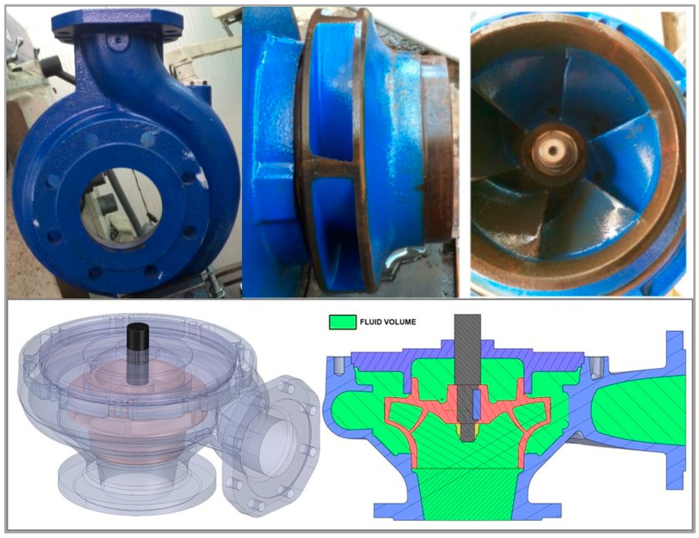
On the top side of
Figure 1, the disassembled pump with a
NS = 37.6 is shown. This pump is a shrouded one with one- channel impeller and six blades and is called Pump 1. Starting from the real geometry in a .step format, the fluid volume has been extracted. In
Figure 1, the fluid-volume is colored in green while the solid impeller is in blue and the solid rotor in red. In the same way, fluid volumes of others two pumps have been extracted and then modelled using a 3D-CFD approach.
The study has been approached using the commercial code PumpLinx
®. PumpLinx
® is a three-dimensional CFD software developed by Simerics Inc. (1750 112th Ave NE, Ste C250, Bellevue, WA 98004, USA) [
25,
26,
27,
28,
29]. It numerically solves the fundamental conservation equations of mass, momentum and energy and includes robust models of turbulence and cavitation.
The fluid volume of each pump has then been meshed with the PumpLinx
® grid generator using a body-fitted binary tree approach. These grids have been demonstrated to be extremely accurate and efficient [
25,
26,
27,
28,
29]. In fact, the parent-child tree architecture allows for an expandable data structure with reduced memory storage, the binary refinement is optimal for transitioning between different length scales and resolutions within the model, the majority of cells are cubes, and, since the grid is created from a volume, it can tolerate inaccurate CAD surfaces with small gaps and overlaps. It is important to underline that, cells are hexagonal not deformed therefore the skewness is zero [
30].
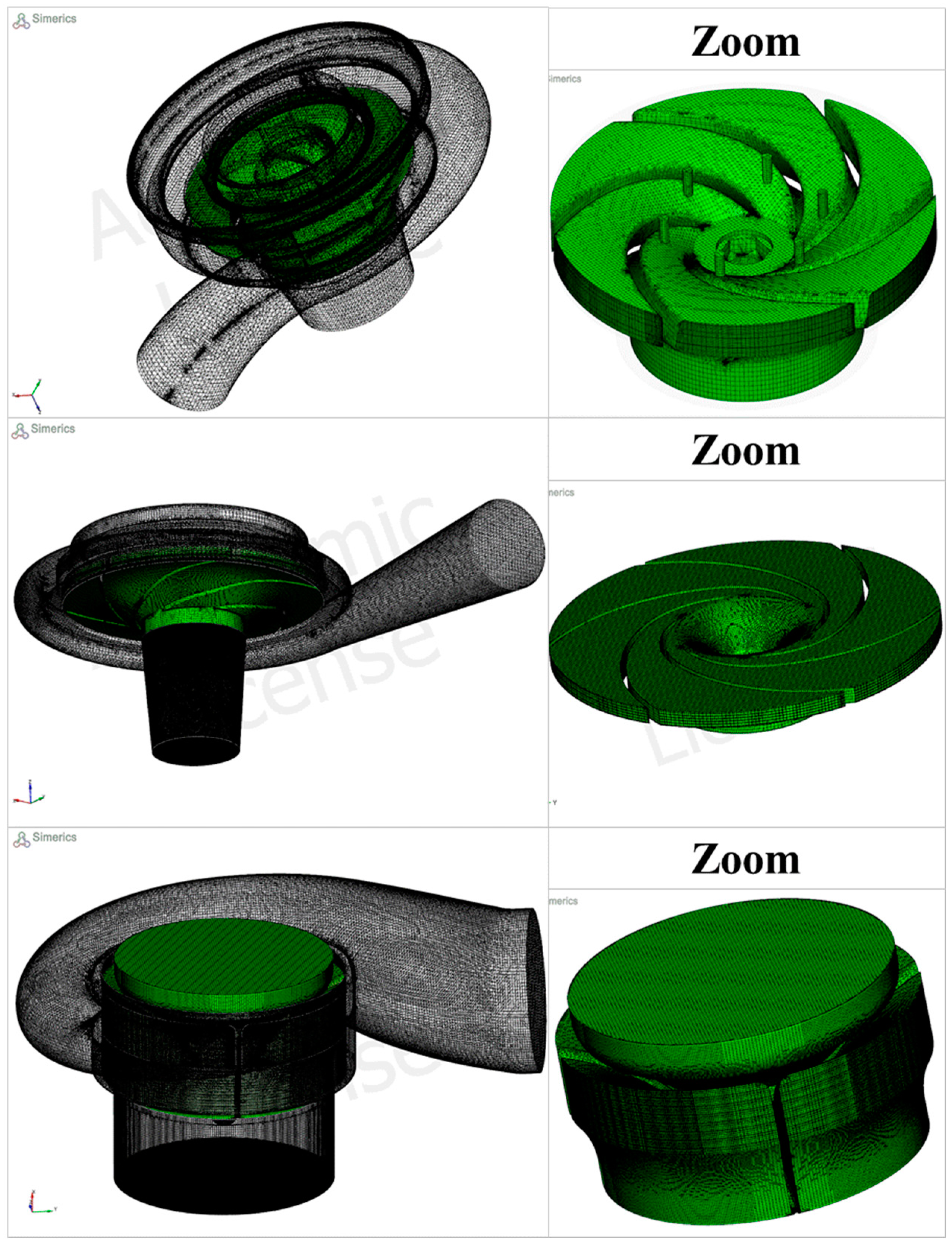
Figure 2 shows the binary tree mesh of three pumps under study: Pump 1 (
Ns = 37.6), Pumps 2 (
Ns = 20.5) and Pump 3 (
Ns = 64).
It is important to underline that using the binary tree approach in the boundary layer can easily increase the grid density on the surface without excessively increasing the total cell count. In this way, the grid has been subdivided and cut to conform it to the surface in regions of high curvature and small details [
27]. Impellers and rotors fluid volumes of each model have been meshed separately. A maximum cell size of 0.025 has been chosen, where no cell in the volume can have a cell side larger than the maximum cell size. The minimum cell size has been fixed at 0.0001. The minimum cell size is a parameter used to limit how small cells can be in attempting to resolve the geometry using the general mesher. No cell in the volume can have a cell side smaller than the minimum cell size. The cell size on surfaces has also been fixed at 0.00625. This parameter is used to control the size of the cells for all surfaces of a mesh volume. Using a pure Eulerian approach the mesh of rotors is deformed by squeezing and expanding the cells. The rotor mesh is colored in green in
Figure 2.
A mesh sensitivity, as well known, is fundamental in studying any new problem with a CFD solver. The target is to allow excellent accuracy (in comparison with experimental tests) and computational efficiency. Pumps fluid volumes have been meshed increasing and decreasing the already described parameters: maximum cell size, minimum cell size and the cell size on surfaces. For each case the best compromise between results accuracy and computational time has been found and by following all mesh characteristic are listed:
- PUMP 1 (NS = 37.6):
Total number of cells: 851.673
Total number of faces: 3.383.745
Total simulation time: 8.9 h as Pump, 9 h as PAT
- PUMP 2 (NS = 20.5):
Total number of cells: 1.039.450
Total number of faces: 3.926.412
Total simulation time: 4.2 h as Pump, 4.8 h as PAT
- PUMP 3 (NS = 64):
Total number of cells: 324.596
Total number of faces: 3.348.318
Total simulation time: 4.5 h as Pump, 4.8 h as PAT
Simulations have been run with an Intel(R) Xeon(R) CPU 2.66 GHz (two processors). It is important to underline that models are transient, and during simulations there is a simultaneous treatment of moving and stationary fluid volumes. In particular, each volume connects to the others via an implicit interface. Mismatched grid interfaces can identify overlap areas and match them without interpolation. These faces, during the simulation process, are treated no differently than an internal face between two neighboring cells in the same grid domain.
Using the models described it has been possible to study the internal fluid dynamics of each pump working in the direct (as pump) and reverse (as turbine) modes. A mature turbulence model has been implemented. It has been demonstrated that for these applications one of the more accurate model to study turbulence is the
k–ε model and RNG
k–ε model. Other turbulence models, such as LES and RNG
k–ε model, might also provide good results but the adoption of higher order turbulence models would have increased the computational time with no relevant improvement of the results. Authors have also applied the presented strategy confirming the solution accuracy [
25,
26,
27,
28,
29,
31,
32,
33] in other analyses.
Therefore, in this research, the
k-epsilon model has been used providing a good accuracy and computationally efficiency. This model is used by the adopted CFD code since it has been available for more than a decade and has been widely demonstrated to provide good engineering results for a wide range of applications [
29,
31,
32,
33]. The standard
k–ε model, used for the simulations presented in this paper is based on the following two equations [
25,
26,
27,
28,
29,
31,
32]:
where
c1 = 1.44,
c2 = 1.92, σ
k = 1, σ
ε = 1.3, where σ
k and σ
ε are the turbulent kinetic energy and the turbulent kinetic energy dissipation rate Prandtl numbers.
The turbulent kinetic energy,
k, is defined as [
25,
26,
27,
28,
29,
31,
32,
33]:
where
v’ is the turbulent fluctuation velocity, and the dissipation rate, ε, of the turbulent kinetic energy is defined as [
25,
26,
27,
28,
29]:
In which the strain tensor is [
29,
31]:
with
ui’ (
i = 1, 2, 3) being components of
v’.
The turbulent viscosity μ
t is calculated by [
16,
23,
24,
32,
33]:
with
Cμ = 0.09.
The turbulent generation term
Gt can be expressed as a function of velocity and the shear stress tensor as [
16,
23,
24]:
where
is the turbulent Reynolds stress, which can be modelled by the Boussinesq hypothesis [
15,
16,
23,
24,
32,
33]:
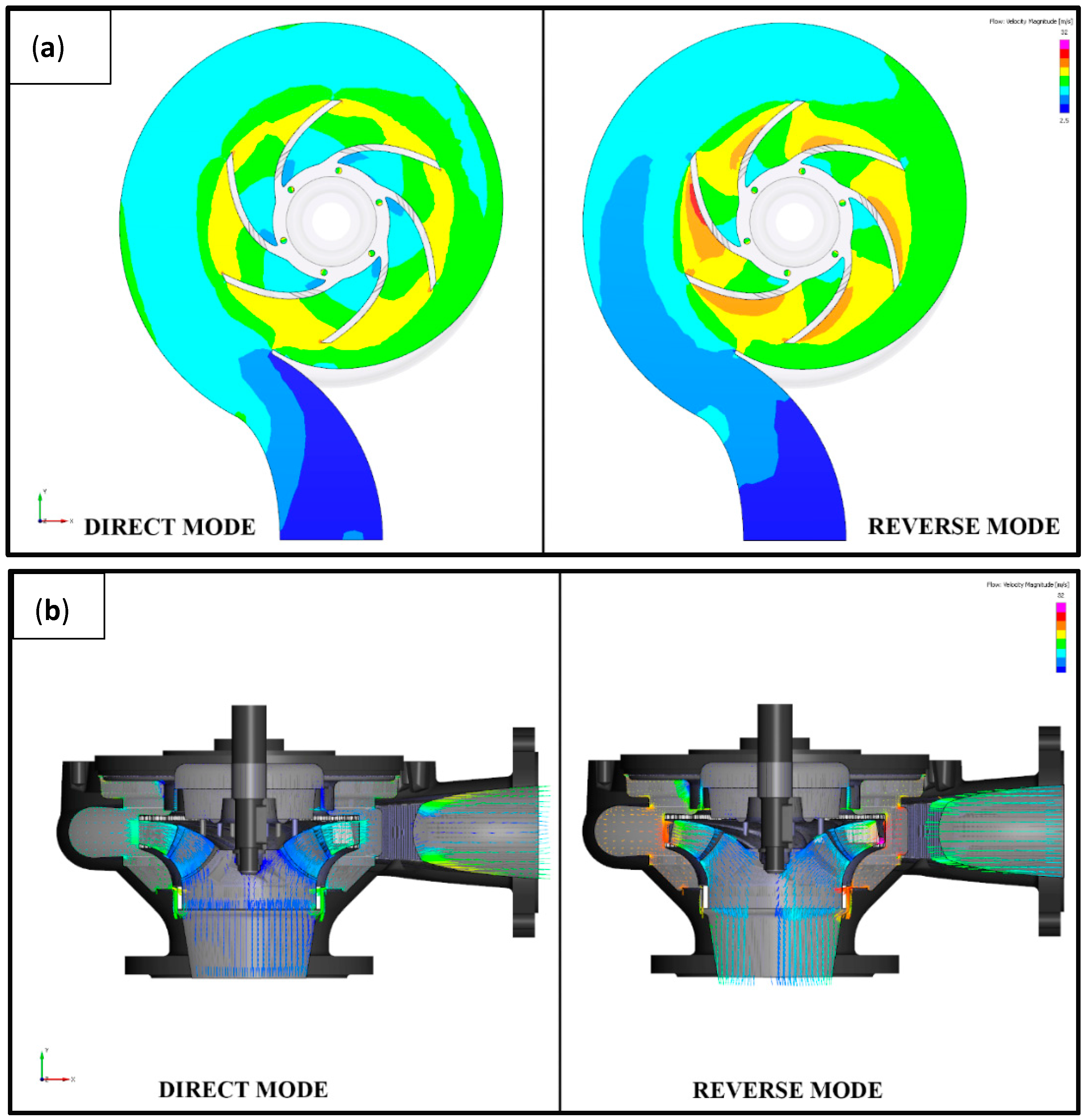
With the built models, simulations have first been run comparing the results in the direct and reverse working modes. Model results for Pump 1 at 2900 rpm are shown in
Figure 3; in
Figure 3a the pressure distribution at the BEP in the 0–9 bar pressure range is presented. The fluid properties of water have been used in all the simulations.
Figure 3b shows the velocity vectors in the fluid volume; the velocity range (0–32 m/s) is the same for the direct and reverse modes. In this picture, it is possible to visualize the flow evolution inside the machine and the acceleration/deceleration of the fluid. Both figures confirm that the velocity is higher in the reverse mode.
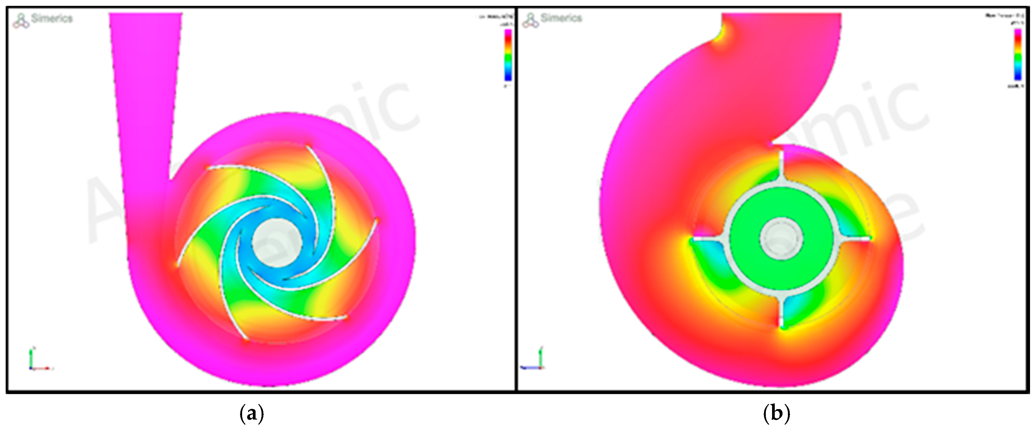
Similarly,
Figure 4 shows the pressure distributions for pump 2 (
NS = 20.5) and pump 3 (
NS = 64) at 2900 rpm.
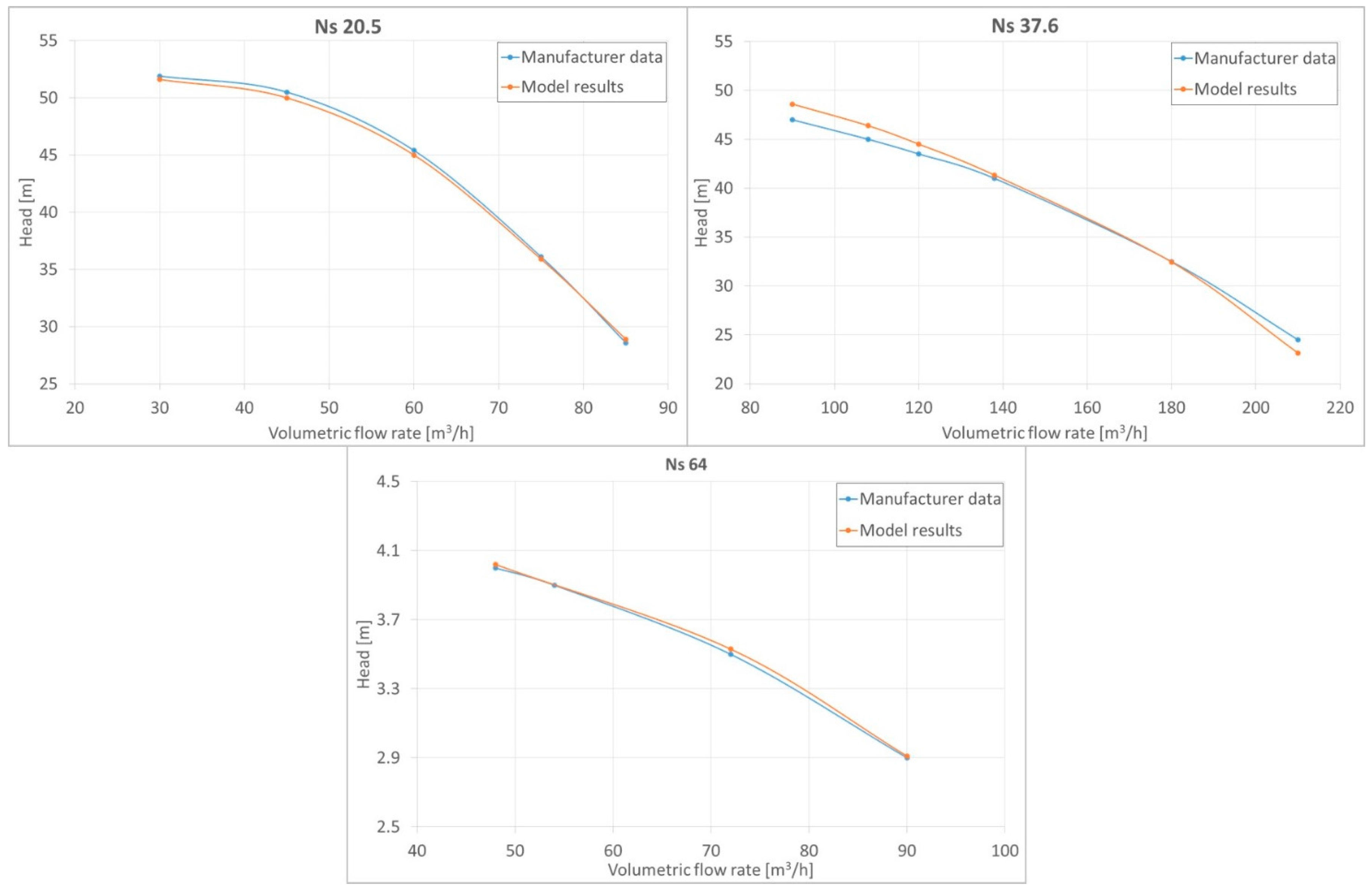
For the direct mode, CFD models have been validated using the data supplied by the pump manufacturers. In
Figure 5, the head vs. flow rate plots (as the blue curves) are shown. Across the range of flow rates (30–207) m
3/h, the head varies from 47 m to 3 m. In the plots in
Figure 5, the model results are shown in red. The comparison in
Figure 5 demonstrates the accuracy of the adopted methodology; in fact, the percentage error is always less than 4% while for many points the error is near zero.
4. Ns 37.6 Pump Model Validation with Experimental Data
Once the model had been validated in the pumping mode, it was decided to also validate it in the reverse mode, to assess whether the model reproduces the turbine mode well. Because the proposed methodology is based only on the results of the CFD model under reverse conditions, the validation under reverse conditions was necessary to confirm the entire methodology.
The model of centrifugal Pump 1 has been validated with data from an experiment performed on a dedicated test bench of the Department of Civil Construction and Environmental Engineering of the University of Naples Federico II. The bench enables testing a centrifugal pump running in reverse mode. The aim of this activity was to further validate the simulation model under reverse conditions. The test bench reproduces a full-scale hydraulic network, made up of four nodes (
Figure 6). An external pump increases the water pressure to simulate the behavior of a real urban network while an air chamber stabilizes the flow rate. The tested pump has been installed in one node where two pressure-reducing valves (PRV) regulate the water flow rate and the pressure at the inlet and outlet of the pump. The pressure is regulated with a valve installed at the network inlet, while the flow rate at the outlet is varied with a butterfly valve. Valves are remotely controlled with electronic actuators controlled by a dedicated homemade software program, with an external PLC [
34,
35,
36,
37,
38,
39,
40].
The electric motor of the pump is linked to an inverter and the produced electrical power is connected to the urban power grid. In the node, two pressure transducers, P1 and P2 (Burkert® model 8314), and a flow meter Q (Siemens® mag 500) have been installed. All test bench data have been acquired by a homemade acquisition system. Furthermore, a 360-tooth encoder has been installed on the electrical motor to acquire the shaft speed.
The hardware system is based on a data acquisition board NI DAQ Card (12-bit ADC converter resolution, 16 input channel, two 24 bit counters), a 68-pin shielded desktop connector block (NI TBX-68). NI LabView performs a homemade software.
The pressure is acquired with Buckert transducers. Sensors are installed upstream and downstream of the PAT, as it is shown in
Figure 6. The characteristics of the pressure transducers are as follows:
Ceramic technology
0–10 bar pressure range
±0.25% accuracy
2 ms response time
The electric motor shaft speed is acquired with a BAUMER BHK 16.05A.360-I2-5 incremental encoder, with 360 teeth, while, as already said, the flow rate is measured with an electromagnetic Siemens mag 500 transducer, (accuracy 0.25%, response time 1 s). The sample frequency was 1 Hz.
The experiments have been performed only in steady-state conditions, varying the water flow rate and the pressure at the inlet of the pump, for different shaft speeds. In particular, the flow rate has been varied between 8 and 21 L/s, and the shaft speed between 300 and 2200 rpm. During the test, pressure at the inlet and outlet of the pump have been acquired at a sample frequency of 1 Hz.
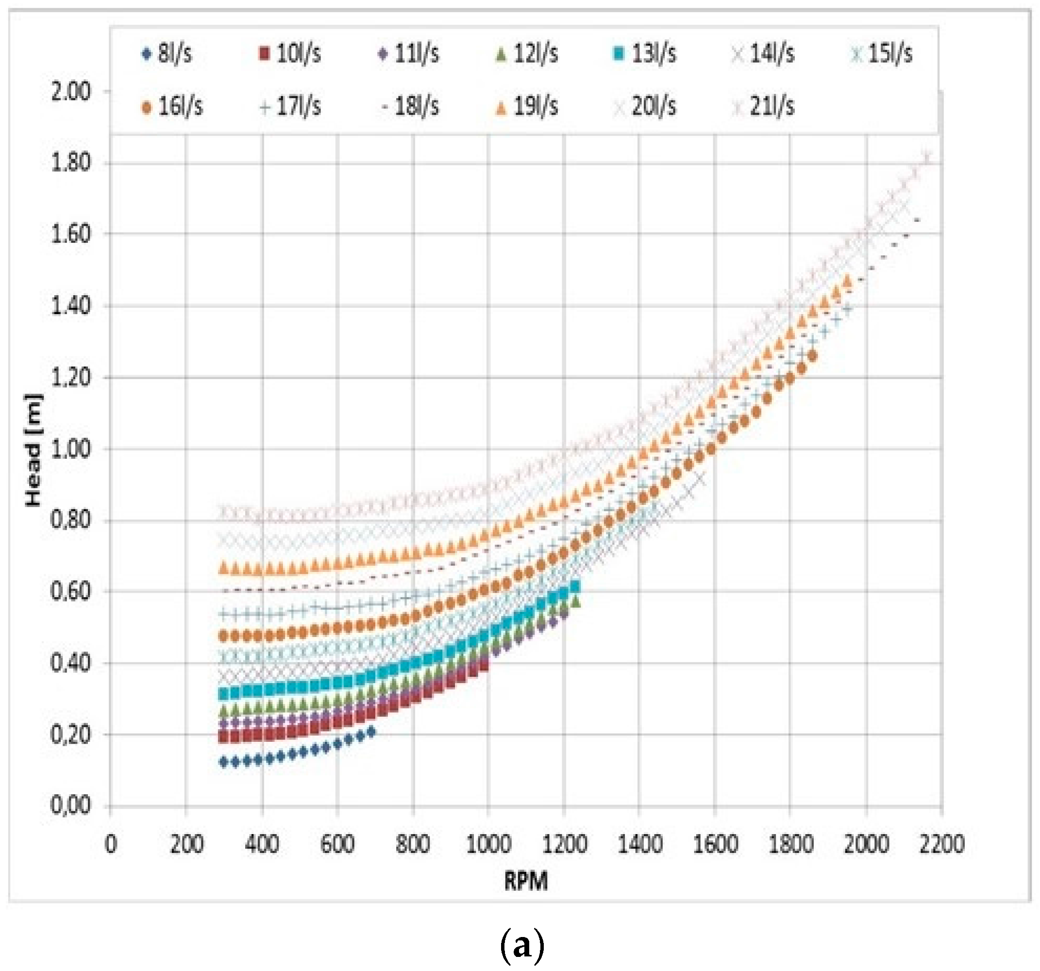
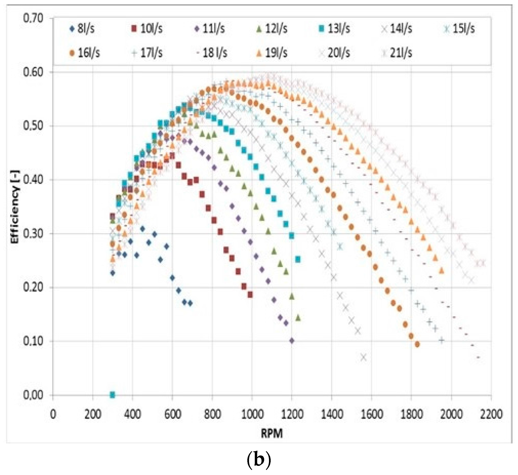
As stated above, the tests have been done in steady-state conditions, running the pump in reverse mode. The flow rate, the pressures at the inlet and outlet of the pump and the shaft rpm were measured. In
Figure 7, all results of the experimental campaign are shown.
To examine the PAT performance, the total head (m) versus shaft rpm is reported, varying the water flow rate for all the examined conditions. Results confirm what is known from the literature: the PAT head increases with the rpm and with the flow—rate, and it can be easily noted that, for the tested conditions, the head varies between 0.1 and 1.8 m.
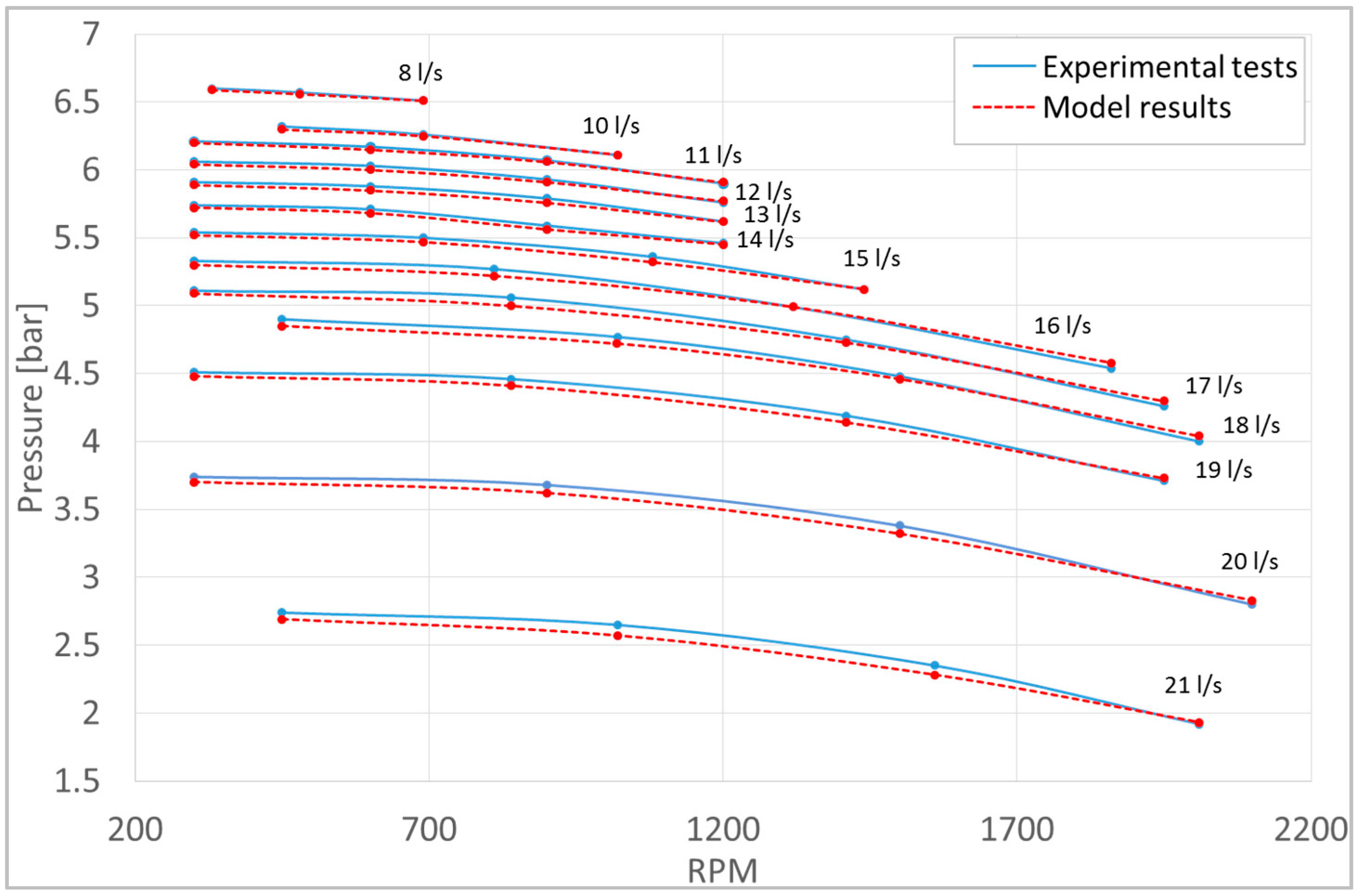
In
Figure 8, the whole validation of the simulation model is presented: it shows that the model reproduces the experimental data well with very small differences between the experimental and the model results for all the running conditions that were analyzed.
5. Model Results
After the validation phase in pump and turbine mode, simulation models have been used to predict the efficiency curves of the three analyzed pumps. Then, all the simulations have been performed to obtain the data necessary to evaluate the inverse characteristics.
The specific head
can be evaluated as:
The specific capacity
depends by the flow
Q and the impeller diameter
D:
The specific power is defined as:
While the efficiency can be evaluated as:
where
H (m),
Q (m
3/s), and
P (W) are the head, flow rate and power, respectively. The rotational speed is
n (RPS) and
D (m) is the impeller diameter. In the reverse mode simulation, the boundary conditions in pump and PAT mode were the same (declared data in pump mode). The boundary conditions in reverse mode are summarized in
Table 2.
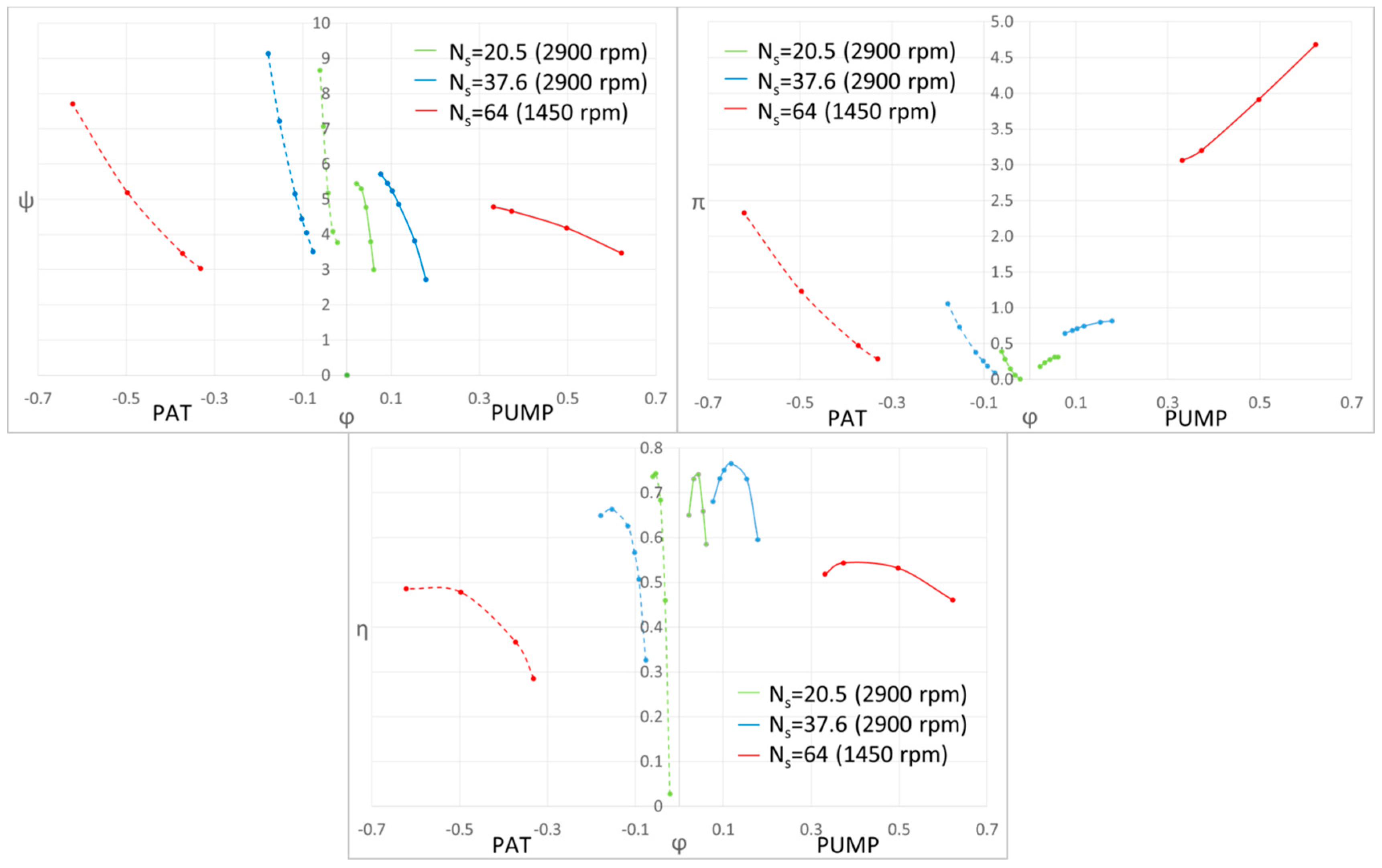
The specific head, the specific power and the efficiency have been evaluated for both pump and turbine mode and for all the studied pumps. These are plotted versus specific capacity in
Figure 9.
It is clear that at high capacity the specific head in reverse mode is always higher than in direct mode. In reverse mode, pumps have a larger power range than in direct mode. The trends are quite different and the curves arising at low flow rate and at higher capacities have a higher power value than in direct mode. In pump mode, the efficiency has a typical “bell shape” while in PAT mode its profile resembles that of a Francis turbine: it increases at low flow rates and reaches a maximum value at high flow rates. Moreover, the pump with the low specific speed works with low flow rates but high heads in direct mode. In reverse mode at high flow rates, the head is higher than the direct-mode value. The pump with the high specific speed works at high flow rates but low heads. In reverse mode, working with the same flow rates, the maximum head is also higher than the direct-mode value. For all pumps, the maximum value is lower than the direct-mode value. For low specific speed pumps, this maximum value is approximately equal to the direct-mode value, while for high specific speed pumps, it is lower.
In conclusion, in
Table 3, the BEP values are summarized:


