Survey on Approximate Computing and Its Intrinsic Fault Tolerance


1
Universidade Federal do Rio Grande do Sul (UFRGS)-Institute of Informatics, Porto Alegre 90040-060, Brazil
2
Ecole Centrale de Lyon-Lyon Institute of Nanotechnology, 69130 Lyon, France
*
Author to whom correspondence should be addressed.
†
These authors contributed equally to this work.
Electronics 2020, 9(4), 557; https://doi.org/10.3390/electronics9040557
Submission received: 20 February 2020
/
Revised: 19 March 2020
/
Accepted: 23 March 2020
/
Published: 26 March 2020
(This article belongs to the Special Issue Approximate Computing: Design, Acceleration, Validation and Testing of Circuits, Architectures and Algorithms in Future Systems)
Abstract
:This work is a survey on approximate computing and its impact on fault tolerance, especially for safety-critical applications. It presents a multitude of approximation methodologies, which are typically applied at software, architecture, and circuit level. Those methodologies are discussed and compared on all their possible levels of implementations (some techniques are applied at more than one level). Approximation is also presented as a means to provide fault tolerance and high reliability: Traditional error masking techniques, such as triple modular redundancy, can be approximated and thus have their implementation and execution time costs reduced compared to the state of the art.
1. Introduction
Approximate computing has been proposed as an approach for developing energy-efficient systems [1], saving computational resources and presenting better execution times, and has been used in many scenarios, from big data to scientific applications [2]. It can be achieved from a multitude of ways, ranging from transistor-level design to software implementations, and presenting different impacts on the integrity of the hardware and the quality of the output. Many systems, however, do not take precision and accuracy as an essential asset. Those are the ones that can profit from this computational paradigm [3].
Even on systems where quality and accuracy are essential, the mere definition of a good quality result can be malleable. On image processing, for instance, the final output is evaluated through human perspective (the quality of the image). This perspective is subjective: Some people are more capable of analyzing the quality of an image than others, and the definition of a “good enough” quality is even more debatable. Typical error-resilient image processing algorithms can indeed accept errors of up to 10% [4], which would be unacceptable for a military system calculating the trajectory of a ballistic projectile. However, this margin of error acceptance can be exploited to improve energy consumption and execution performance.
The weak definition of “error acceptance” can also be used by approximate computing for quality configuration. Given that different systems have different quality requirements, a designer might make use of just the necessary energy, hardware area, or execution time, to meet the needs of his project. An excellent example of how a circuit can be configured in that manner is by using different refresh rates for memories [5], or different precision for data storage and representations [6]. The image processing domain is particularly interesting because it is an example of how approximation can be implemented on different levels. A minor loss in precision can be accepted by applying approximation via hardware, by reducing the refresh rates of eDRAM/DRAM and the SRAM supply voltage, which reduces energy consumption [7]. On a higher level of implementation (i.e., at software level), the approximation can be used by loop-perforation (finishing a loop execution earlier than expected) [8] or by executing specific functions on neural accelerators [9].
The common point among the above-listed approximation techniques is the reduction of the “intrinsic reliability” of the application. Thus, the hidden cost of approximation techniques is the reduction of the inherent fault tolerance of the application itself [10]. This cost has never been quantified and taken into account as a metric by approximation techniques. However, it must be considered specifically when the approximated application runs on a safety-critical system. Safety-critical systems often deal with human lives and high-cost equipment and therefore shall provide high dependability. Those systems are constantly subject to faults, given the dangerous environment they are subjected (e.g., radiation for aerospace systems). When a fault affects the system in a way that is perceived by the user or other parts of the system, we say that an error occurs [11]. A soft error occurs when it does not permanently damage a system. A soft error is also called a single event upset (SEU). In some cases, such as when there is exposure to intense radiation environments, electronic systems are affected by multiple bits upset (MBU), but those cases are rare.
Various methods for approximation and their impacts will be presented in the next section. Furthermore, the implementation of approximation on safety-critical applications is also discussed.
2. Approximation Methods and Their Impacts
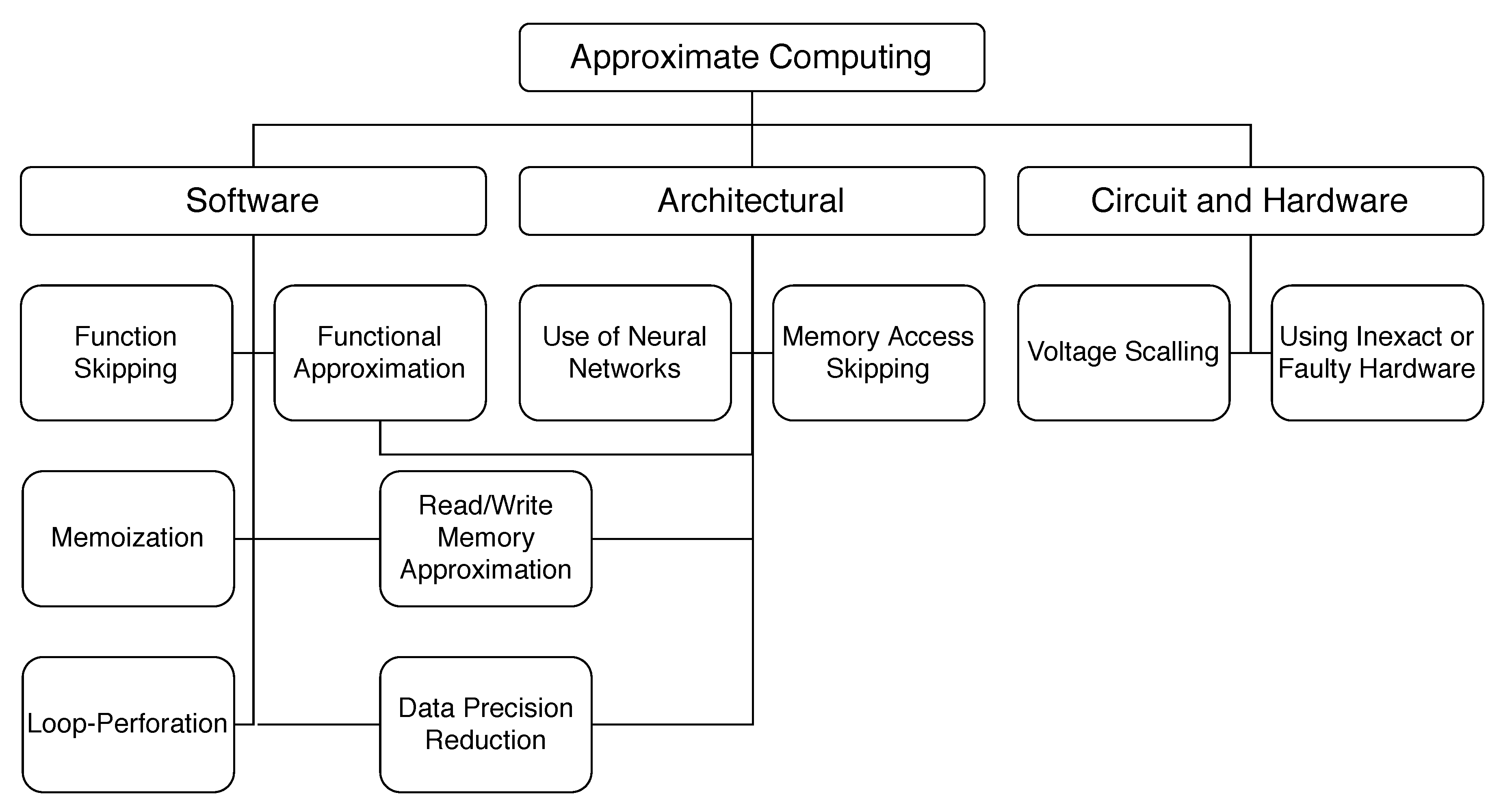
Approximation techniques can be applied to all the computation stack levels. Figure 1 divides approximation techniques into three groups that define their implementation level: Software, architecture, and hardware. As Figure 1 shows, some approximation methods can even be implemented on more than one level. Load value approximation, for example, can be both implemented by purely software approaches or at memory control units. Figure 1 presents only some of the most used approximation methods and the most discussed in the literature. However, there are uncountable ways of approximating an application, and the very definition of what is to be considered an approximation or not is debatable.
The loop-perforation technique is an excellent software approximation example, being able to achieve useful outputs while not executing all the iteration of an iterative code. Similarly, task-skipping consists of skipping code blocks during run-time following previously defined conditions. Another approximation technique for software applications consists of reducing the bit-width used for data representation. This technique impacts mainly the memory footprint of the application. Indeed, data precision reduction can also impact the execution time performance of the software, but that would depend on the hardware implementation of operations in use by the application. Hardware-based approximation techniques usually make use of alternative speculative implementations of arithmetic operators. An example of this approach is the implementation of variable approximation modes on operators [12]. Hardware approximation is also present in the image processing domain in the form of approximate compressors [13].
The techniques presented in Figure 1 are presented in detail and with implementation examples below:
- Function Skipping: In a system composed of tasks that complement each other in the sense of providing a final result, some of the tasks can be skipped while maintaining a level of accuracy and error resiliency defined by the user [14];
- Memoization: Traditionally, memoization consists of saving outputs of functions for given inputs to be reused later. Given that some input data are frequently reused, their calculated outputs can be stored and used without the need for the re-execution of the function. Memoization can also be used to approximate applications, if similar inputs provide similar outputs for a given function, it means that the already-calculated function output can approximately cover a range of inputs. In [15], the authors propose approximate value reuse for memoization, providing a very low accuracy loss;
- Loop-Perforation: In loop-based algorithms, loop-perforation can be used to highly reduce the execution time. An excellent example of this type of application is numerical algorithms. The calculation of an integral using the trapezoidal method, for example, consists of calculating the area of a high number of trapezoids under the curve of a function, providing an approximation of the area beneath it. Reducing the number of calculated trapezoids, the final value will be less accurate, but the program will finish earlier. The literature also presents techniques to apply this approximation method on general-use algorithms, filtering out the loops that cannot be approximated and using loop-perforation on those that can [8]. Authors claim that their approach typically delivers performance improvements greater than a factor of two while introducing an output deviation of less than . Loop-perforation is an algorithm-based approximate technique, as it is only applicable to loop-based code, which limits its applicability. It can be implemented both at software and programmable hardware code. The difference is that, on programmable hardware, a loop might be implemented either as many circuits executing in parallel (one being each iteration of the loop) or one circuit that is re-executed in a timeline. Therefore the impact of loop-perforation on software and hardware implementations can be very different. On software, it will mainly impact the execution time of the application, while in a FPGA implementation, it could also affect the energy and area consumption;
- Functional Approximation: Some systems are composed of components that do not need to provide accuracy as much as others. The idea is to take advantage of the fact that even inside an algorithm, some components affect less the final accuracy than others. Those components can be approximated to provide energy consumption reduction and improve execution time performance [16]. On the architectural level, functional approximation can appear as alternative speculative implementations of arithmetic operators. An example of this approach is the implementation of variable approximation modes on operators [12]. When applied to software applications, approximate computing usually consist of inexact computations, which provide results with lower accuracy than usual [17]. Most approximate computing techniques for software consist of modifying the algorithm so that it executes approximately, providing a final result more rapidly. One of the problems with functional approximation is that it introduces error on the system output that may be too big to be acceptable. The works at the architectural level of approximate operators [12], for example, that do not present a significant hardware implementation area reduction when compared to a traditional operator. The size of the used area on programmable hardware devices has a direct impact on system reliability [18]. Therefore, the quality loss (in this case manifested as errors in some operation results) introduced by the approximation would only be acceptable by safety-critical systems if it sharply reduced its area;
- Read/Write Memory Approximation: It consists of approximating data that is loaded from or written in to the memory, or the read/write operations themselves. This is primarily used on video and image applications, for example, where accuracy and quality can often be relaxed, to reduce memory operations [19,20]. In [6], the authors propose a technique that uses dynamic bit-width based on the application accuracy requirements, where a control system determines the precision of data accesses and loads. The authors claim that it can be implemented to a general-processor architecture without the need for hardware modifications by communicating with off-chip memory via a software-based memory management unit. Approximation can also be applied to the cache memory. In the event of a load data cache miss, the processor must fetch the data from the following cache level, or at the main memory. This can be a very time-consuming task. Load value approximation can be used to estimate an approximate value instead of fetching the real one from memory. In [21], the authors present a technique that uses the GPU texture fetch units to generate approximate values. This approximation causes an error of less than in the final image output while reducing the kernel execution time in . In [22], the authors propose an approximation technique for multi-level cell STT-RAM memory technologies by lowering its reliability up to a user-defined accuracy loss acceptance. This memory technology has a considerable reliability overhead, which can be reduced. They selectively approximate the storage data of the application and reduce the error-protection hardware minimizing error consumption;
- Data Precision Reduction: Data precision reduction is one of the techniques that can be implemented both at a software and architectural level. Reducing the data precision of an application (i.e., the number of bits used to represent the data) is a straightforward technique to reduce memory footprint. Reducing memory usage also reduces energy consumption at the cost of accuracy (i.e., less data have to be transferred from/to the memory). In [23], the authors show that reducing floating point precision on mobile GPUs can bring energy consumption reduction with image quality degradation. This degradation, however, can be acceptable and even unperceivable for the human eye. Lower memory utilization is suitable for safety-critical systems because it reduces the essential and critical bit count, making them less susceptible to faults. Reducing the bit-width used for data representation is also a popular approximation method [24]. The way data precision reduction can be used to approximate software and FPGA applications is obvious: It is a matter of code modification. In software, the precision of floating-point units can be easily modified with the use of dedicated libraries, or even by merely changing the type of the variable. The same can be done at VHDL/Verilog projects: A design can be adapted to process smaller vectors of data. Data precision reduction can bring good improvements in area and energy costs for hardware projects, but frequently do not present high costs reduction on software. Fixed-point arithmetic, for example, can be used to approximate mathematical functions, such as logarithm, on FPGA implementations providing low area usage [25]. On software, however, it can increase the execution time of the application because all the operations and data handling routines are implemented at the software level;
- Use of Neural Networks: A neural network can learn how a standard function implementation behaves in relation to different inputs via machine learning. In a complex system, the neural network can be used to implement approximate functions via software-hardware co-design. Traditional approximable codes can be transformed into equivalent neural networks that present a lower output accuracy but better execution time performance [26];
- Memory Access Skipping: Using a combination of the memoization and function skipping techniques, it is likewise possible to skip memory accesses. Uncritical data can be omitted, as long as it will not heavily damage the output accuracy. Approximate neural networks can skip reading entire rows of their weight matrices as long as those neurons are not critical, reducing energy consumption and memory access, and improving performance [27];
- Voltage Scaling: The supplied voltage level can be scaled at the circuit level, impacting the computation timing of processing blocks inside the clock period. It affects the accuracy of the final result and also energy consumption [28]. In [28], the authors propose the voltage overscaling of individual computation blocks, assuring that the accuracy of the results will “gracefully” scale with it. Voltage scaling can be implemented in hardware dynamically. Dynamic voltage and frequency scaling (DVFS), for example, is a power management technique used to improve power efficiency, reducing the clock frequency, and the supply voltage of the processor [29]. DVFS can cause data cells to be stuck with a specific value because it diminishes the threshold between a logical one and zero. This type of approximation impacts the integrity of the hardware and the precision of the data. The voltage scaling technique can be applied at both the processor architecture level and programmable hardware. At the architectural level, voltage scaling is implemented during the design of the circuit. Most FPGA manufacturers make the voltage scaling of the device possible through easy-to-use design tools. Even though it will impact the performance of a software application, it is not part of the software approximation group because its implementation has no direct connection with software development;
- Using Inexact/Faulty Hardware: Inexact and faulty hardware can be used at the architecture level to provide an approximation. The literature presents a multitude of approximate adders proposals. One approach is to remove the carry chain from the circuit to reduce delay and energy consumption. This can be done by altering the subadders of a standard adder cell of n bits [30]. In [31], the authors presented an approximate multiplier design that gives correct outputs for 15 of the 16 possible input combinations and uses half of the area of a standard non-approximate multiplier.
As we can see, approximation techniques can be implemented not only in all the computation stacks but also in many abstraction levels. The functional approximation is an example of a technique that can be applied at the software and architectural computation stacks, and implemented via software code modification, programmable hardware, and even on a circuit level. Loop-perforation can also be achieved via code modification for embedded software and programmable hardware (using high-level synthesis, HLS), or directly with HDL project modifications. The way the approximation techniques are technologically implemented also has a considerable impact on their performance. Approximate computing at the software level is less presented in the literature than it is at the hardware level. This is probably due to the origins of approximation being on energy consumption reduction and neural network applications.
Developing alternate approximate versions of an algorithm is a very time-consuming and intellectually demanding work. To deal with this issue, some works propose frameworks that identify approximable portions of code. At [32], the authors present a framework to discover what are the data that can be approximated without significantly interfering with the output of the system. They do so by injecting faults in the variables and analyzing how they affect the quality of the output. Another method is to identify parts of application code that can be executed on approximated hardware, saving resources and energy [33]. The type of approximation to be applied to the approximable parts of the application would depend on the application in question and project requirements. Although those frameworks are presented as general-use, the question remains if they really can be applied to every type of algorithm. As they base their methodology on simulation, it is hard to believe that they are able to cover every possible kind of fault that can affect every system.
Given the plethora of approximation methods and systems that make use of them, the literature also presents an extensive list of error metrics definitions. Metrics can be applied on an application level (e.g., the output image is analyzed) or the system level (e.g., intermediate values are analyzed). Details about each metric can be found in [34]. Some examples of how precision loss is measured on approximate systems are:
- Application-Level:
- -
- Pixel Difference: Consists of a full comparison of two images pixel-by-pixel, where every pixel is represented by a value. Normally used to compare gray-scale images, where the pixel value defines the grey intensity (the higher value being complete darkness);
- -
- Peak signal-to-noise ratio (PSNR): Is calculated using the mean square error (MSE) between the two images (the original and the approximate one), and indicates the ratio of the maximum pixel intensity to the distortion. It is calculated by the formula , where MAX stands for the maximum value of a pixel in the images;
- -
- Ranking Accuracy: When approximate computing is applied to ranking algorithms, such as the ones used by search engines, it can generate different results depending on the ranking definitions and the algorithms used. A research result from Bing and Google search engines, for example, will likely be different. The accuracy is defined based on pre-established parameters.
- System-Level:
- -
- Hamming Distance: When comparing data bit-wise, the hamming distance consists of the number of positions where the bit values are different between binary strings;
- -
- Error Probability: Consists of the error rate of all the possible outputs, comparing the result of an approximate function and its non-approximate counterpart. This metric gives the probability for an approximation to present an error but does not evaluate the criticality or impact of that error;
- -
- Relative Difference: Presents the error in relation to the standard non-approximate output. This metric is capable of evaluating the criticality of an error.
The presented quality evaluation metrics are not mutually exclusive. One application might use several different parameters to evaluate its quality loss. Both PSNR and pixel difference are used as image quality metrics, for example.
Approximation in Practice
Approximation might be unavoidable for some applications. On others, it might present good opportunities to lower hardware costs and improve performance and reliability. The usage of approximation is primarily motivated by three factors:
- Unavoidable Approximation: Some problems can only be computationally solved by approximate algorithms. Floating-point operations, for instance, have frequent rounding of values, making it inherently approximate. Numerical algorithms are also often of approximate nature: The calculation of an integral, for example, is not natural for a computer, and consists of an iterative calculation of a finite sum of terms (and not an infinite one, as the mathematical theory defines it). A practical industrial example is the sensors systems of an airplane, that always provide the pilot with an approximation of environmental values. Numerical algorithms are also by themselves approximations and are often used to calculate areas or trajectories of projectiles by military systems. On many computations, rounding happens very frequently (e.g., the rounding of a number when using trigonometrical functions, or writing data in either single-our double-precision floating-point variable types);
- Quality Configuration: Even some parts of safety-critical systems are not critical themselves and do not call for accuracy, as exemplified above with image processing systems. Indeed, many applications do not need great accuracy. Apart from that fact, those that need a certain accuracy or output quality often have a margin of acceptance. Indeed, the approximation can be configured to provide different levels of accuracy, thus also provoking various levels of impact on the system. The loop-perforation method, for instance, can be configured to provide approximation up to the optimum point that correlates the loop-size, the accuracy of the result, and the execution time. Similarly, data precision reduction can be easily configured as a means to impact the accuracy of the data on different levels. In that case, it would only be a matter of how many bits the binary representation of the variable would lose. A designer could find the best approximation possible, given his accuracy, energy consumption, and hardware usage requirements;
- Error Resiliency: As will be further discussed in this survey, the error resiliency that is inherent to approximate computing is also an important source of motivation to use this computing paradigm.
When implementing approximate computing algorithms on safety-critical systems, one shall keep in mind that criticality is not necessarily related to the system as a whole. A safety-critical system might consist of many parts, and some of them are possibly not critical. Such is the case of an airplane. It is easy to see an airplane as a safety-critical system. However, many parts of that system are not critical, in the sense that a failure affecting those parts would not be catastrophic. A commercial airplane transporting passengers would have, for instance, multimedia and in-flight entertainment systems. Even though a transatlantic travel without those systems would be very dull, a failure affecting the entertainment system of a commercial plane would not put in risk the lives of the passengers. However, approximate computing requires attention to their applicability. Some approximation methods can lower the quality of service at an unacceptable rate. While safety-critical systems can make use of approximation to improve their performance, energy consumption, and even reliability, the sometimes unpredictable behavior of approximate computing algorithms can be dangerous.
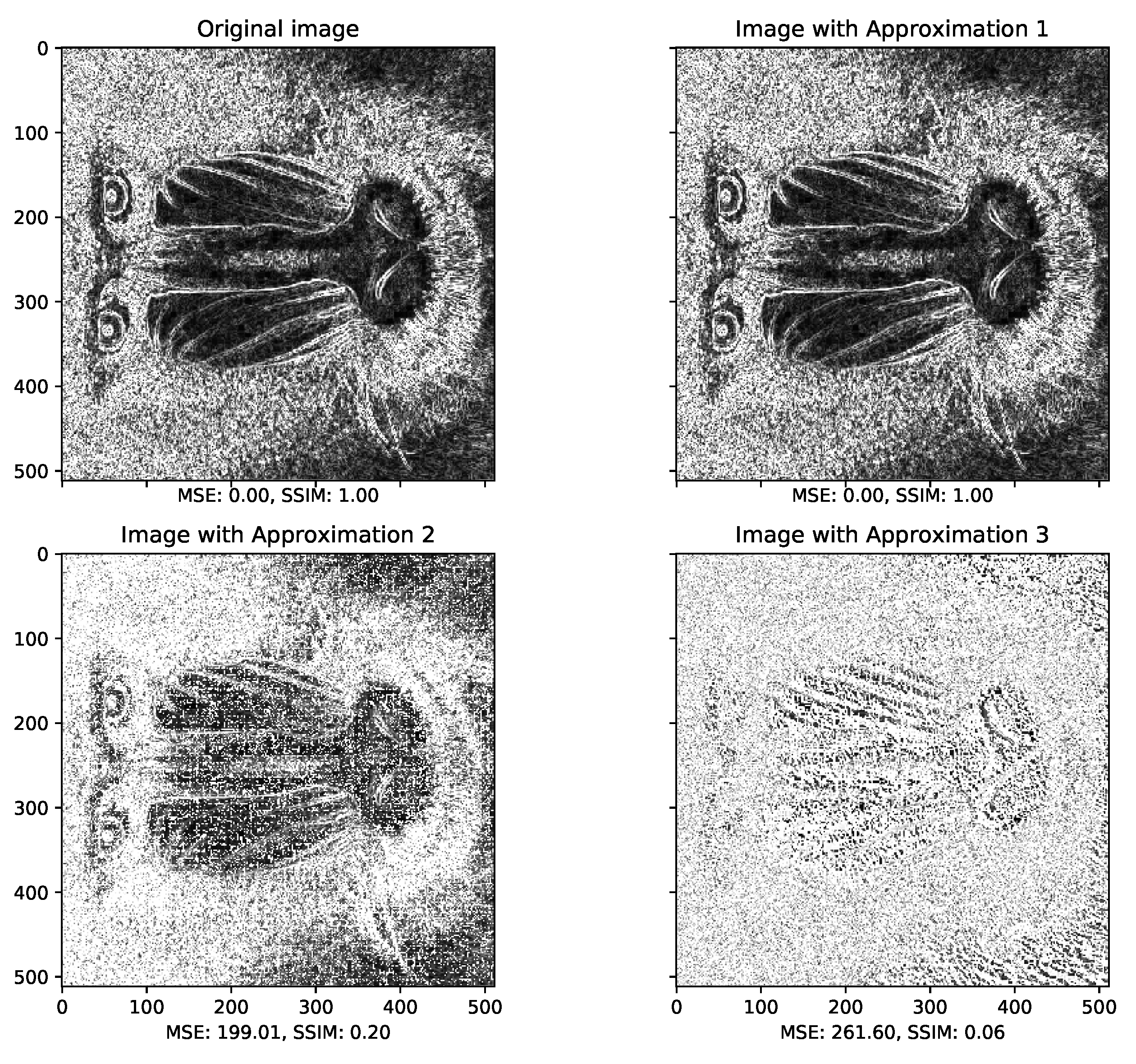
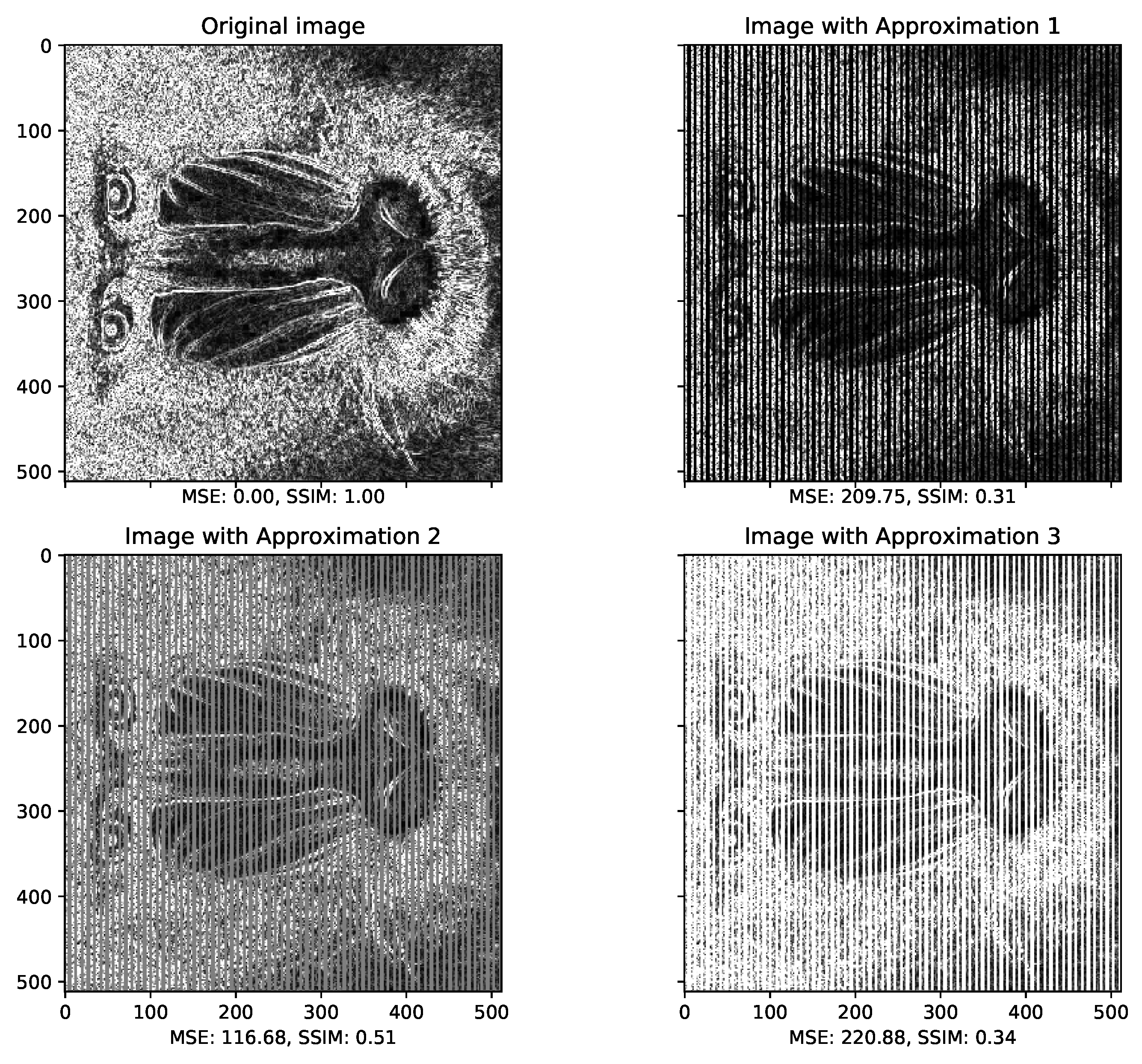
Figure 2 and Figure 3 present examples of outputs from hardware implementations of a Sobel filter. The Sobel filter takes as input an image and finds its borders. The output is a grayscale image, with pixels ranging from the value 0 to 255 (being 0 black and 255 white). Sobel filter is often used in autonomous system (i.e., drone) to pre-process frames coming from sensor camera to extract features for real-time collision avoidance algorithms. Figure 2 presents an implementation that approximates one of the operations using data precision reduction (each approximation contains one less bit than the previous) and function approximation (the operations had to be re-designed to deal with the new data sizes, so we can consider them approximations as well). Figure 3 presents an approximation using loop-perforation. All the approximation examples shown in Figure 3 skip iterations on half of the input image pixels (it can be noticed by the vertical rows that correspond to skipped iterations). The difference among them, is the solution used to fill the missing pixels (i.e., skipped iterations) that is white, black, and gray (i.e., 0, 255, or 127).
It is evident from the example above how approximation, and its intensity, affects the quality of the image output. Figure 2 shows that the output from the first approximation (that reduces the data-size in one bit) is the same as the original one. The second approximation (reducing the data-size of two bits) is already enough to provoke a considerable quality loss. The third approximation provides an image output that is barely recognizable as somewhat related to the original one. The loop-perforation example of Figure 3 shows that this type of approximation implies on different approaches for the output. Naturally, the part of the image that is not processed (because of the loop-perforation) needs to be filled somehow. The example provides three simple solutions for that problem (filling missing pixels with white, gray, or black). It could, however, be solved in much more elegant manners. One option would be to calculate the value of the pixel as (i.e., the mid-value between the previous and the next pixel value). One could also use AI methods to predict possible values to fill the image voids.
Approximate computing algorithms usage on safety-critical systems are also motivated by their error-resilience. The following sections will present this behavior and how it applied to fault tolerance.
3. Approximation and Fault Tolerance
On safety-critical systems, the definition of error is related to the occurrence of a fault, and not to an expected quality deviation caused by the algorithm itself. In this scope, the approximation can be used in two manners. First, it can be used to improve the application execution time, energy consumption, and even reliability. Secondly, approximate computing can also be used to reduce the costs of fault tolerance techniques. The impact of using approximation on those two levels, however, is different. As already discussed, the approximation of the application directly impacts its accuracy, and therefore reliability. Approximating fault tolerance techniques may, however, be developed in such a way to avoid affecting the accuracy of the application, or affecting it only up to the acceptable level that is defined by its quality (or accuracy) requirements.
Approximation itself implies the idea of inherent error tolerance. On approximate systems, a specified error tolerance has to be considered, but that is not the same error definition used when discussing faults and their effects and safety-critical systems. Approximation errors are caused by the system itself and manifested as quality or accuracy degradation. Also, when dealing with approximation, the decision of whether an error caused a failure or not is a matter of definition related to what would be considered a “correct” application output, which is often hard to be defined. Take, for instance, the example of image outputs: The correctness of the output is tied to an image quality definition, which is different from one human being to another because of biological reasons.
The accuracy relaxation inherent to approximate systems can be used in favor of fault tolerance on safety-critical systems. A system that accepts some accuracy degradation can ignore errors in memory that have a low impact on the data value. Also, the reduction of the complexity, achieved by approximation, can help to reduce the system’s susceptibility to faults (e.g., by reducing the critical area of a hardware circuit). Another example of applications that can accept some quality degradation is real-time systems. Those systems have very strict deadlines, requiring strong performance, and dealing with data freshness. Data freshness is the concept that data has an expiration time, being refreshed from time to time and only valid in a given time window (e.g., data coming from a radar system is, from time to time, refreshed and overwritten with new values). In those cases, an error correction procedure is often not necessary, and errors are tolerable when paying the cost for better performance. The error criticality in approximate systems is not related only to the system itself but also the position of a fault (data precision) and the time of the fault.
Redundancy methods such as duplication with comparison (DWC), which duplicates the application and implements a checker to compare any discrepancy between the data generated by the two independent executions, are employed in a multitude of systems, both to provide error detection and masking. DWC is capable of finding errors, but not masking them. A third execution would be needed to mask the error, making a vote for the correct data possible, thus the implementation of triple modular redundancy (TMR). DWC techniques have an overhead of two times the execution time of the original software application for pure redundancy and three times when applying re-execution for error masking. The TMR has, at least, an overhead of three times the execution time of a software application.
When applying a TMR method to approximate algorithms, there is no need to have three tasks with high accuracy. As only one of the outputs will be taken as the final “correct” one, the others can have a lower accuracy (e.g., fewer iterations in the case of loop-perforation approximation). Tasks with lower accuracy and execution time cause lower overhead.
Approximate TMR (ATMR) is based on implementing each redundancy task with a different architecture or algorithm [35]. When applied to hardware projects, ATMR has been presented as a way to achieve fault coverage almost as good as traditional TMR but avoiding the huge area overhead that it costs [36]. Designers might accept a lower fault coverage if the area overhead of the project is to drop significantly. Also, a smaller hardware area implies higher fault tolerance due to the reduction of the critical area. Therefore ATMR might be, in some cases, not only less costly but also more reliable than traditional TMR. In traditional TMR, at least two redundancies need to have the same correct value at a given time so that the correct output can be voted.
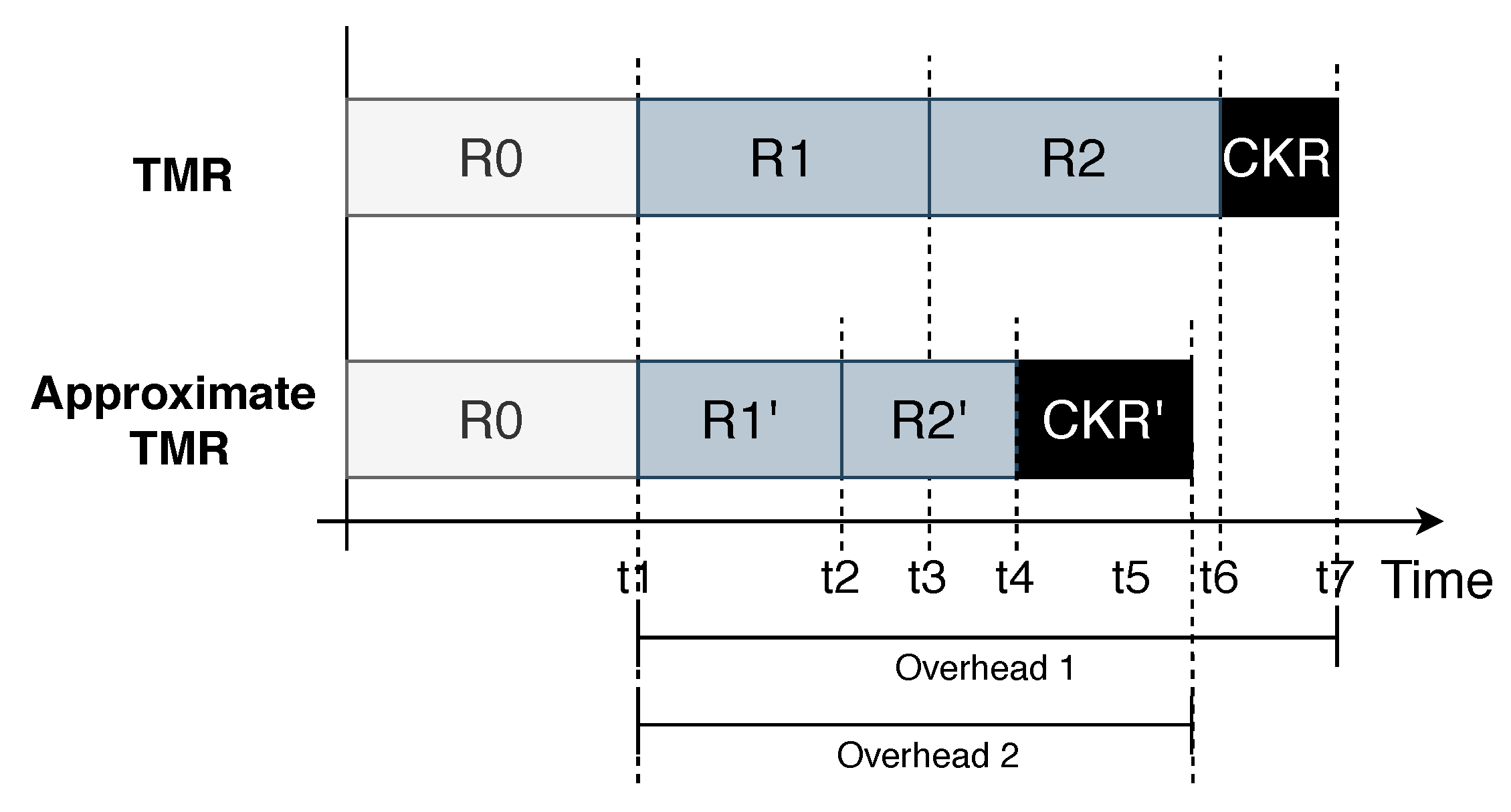
Figure 4 presents an example of the ATMR method. In the figure, R1’ and R2’ are redundant tasks of R0 with fewer iterations, while R1 and R2 are hard copies of R0. Please note that the considered TMR exploits timing redundancy. The redundant tasks (R1, R2, R1’, and R2’) are executed serially after R0. The three results are then compared and voted by the checker. The overhead of a TMR consists of the extra execution time it costs. On the other hand, the overhead of the checker (represented at the figure by the CKR box) is constant. However, reducing the execution time of the tasks, the overhead of the TMR can be lowered. As R1’ and R2’ execute faster than R1 and R2, the ATMR presents a speedup in relation to the TMR.
The approximate checker (CKR’) plays a critical role in the ATMR method. In a traditional TMR, the checker would make a bit-wise comparison between the three outputs, changing every bit that is different from the other two to the same value. However, with approximate computing, the checker needs to be more complex. The value of the three outputs may be different even in the absence of errors, because of the varying accuracy of each ATMR task. To deal with this issue, the ATMR checker has to be programmed in a way to deal with those differences, considering a threshold of acceptable difference between the ATMR output value and the expected golden value. This acceptance threshold might be different for each application or system and impacts the ATMR error masking performance.
4. Approximate Computing Applied to Safety-Critical Systems: A Case Study
Given all the characteristics of approximate computing, it may not be applicable to every system. Some approximate computing methods, such as task skipping and loop-perforation, can present a non-deterministic result accuracy and execution time, depending on their skipping and execution stop conditions, and their stimuli. For example, applying loop-perforation to reduce the number of iterations of the execution of a Newton–Raphson algorithm can improve its execution time at the cost of final result accuracy. The Newton–Raphson algorithm finds the roots of a function calculating the intersection of the tangent line of the function in an initial guess point with the x-axis. It is calculated iteratively, as stated in Equation (1) until it reaches a sufficient accuracy (i.e., the difference between and is minimal):
Newton–Raphson belongs to the successive approximation algorithms class [37]. Among them, physical problems are often described by Partial Differential Equations (PDEs). Since analytic solutions cannot be obtained in general, numerical algorithms are used to find solutions by means of a software implementing (among the others) successive approximation algorithms. Successive approximation algorithms consist mainly of numerical calculations. Those are intended for when an exact solution is not computationally achievable. Some of the most significant mathematical problems (e.g., derivatives and integrals calculations) base their only solutions on successive approximations. Those solutions are of great importance for a significant number of applications and among them, the safety-critical ones [37]. However, depending on the stop condition of the algorithm, the number of iterations is uncertain, which violates the rules of hard real-time systems (on which the execution times of processing tasks need to be well known). This specific example of the Newton–Raphson algorithm, however, demonstrates how an approximation can be adapted to follow the requirements of a certain project.
At first glance, one might say that this algorithm is not convenient for hard real-time systems, given that different functions, with different inputs and different initial points of execution will take different execution times to finish. This, however, can be avoided with a simple adaptation of the program code to limit the number of loop execution to N maximum iterations, given that N shall be defined concerning the maximum execution time defined by the system specification dedicated to the task execution. This modification could, however, impact the quality of the algorithm output in an uncertain way. By limiting the maximum number of iterations of a successive approximation numerical algorithm such as the Newton–Raphson method, there is little to no guarantee that the final computation output would be acceptable inside a given quality metric or even represent any result approximation is lost. This leads to another important limitation of approximate computing and its applicability to safety-critical environments: The level of approximation and its domain. An aggressive approximation can prevent the algorithm from terminating with an acceptable output.
Let us analyze how a successive approximation algorithm such as Newton–Raphson would behave a real case scenario, such as executing inside a safety-critical system, subject to faults caused by external sources. Figure 5 presents the evolution of the Newton–Raphson output concerning the iteration number when affected by faults. The y-axis of the graphs represents the distance between the current computed value and the final best achievable result for the algorithm (i.e., the absolute difference between the two), and the x-axis presents the current number of iterations executed. The algorithm should finish after 14 iterations if no faults were injected. The “No Faults” curve shows the evolution of an execution with no external faults injected. Faults are injected in the memory word that holds the latest computed value (i.e., the output from the last executed iteration), and all faults are injected precisely at the end of the 5th iteration of the algorithm. Each curve presents the progression of the algorithm result with one fault injected in a different bit of the word, as the legend shows. The curves show the apparent tendency for the algorithm to correct itself and end up finding a good result even under external fault injections. In all the cases the algorithm deviated from the expected result evolution curve and took more iterations to finish, but was capable of finding it with no failures.
The inherent fault tolerance of the Newton–Raphson algorithm is also expressed in Figure 6. The data presented in this figure is from the same fault injections presented in Figure 5. The difference is that it now shows the impact of injecting faults on various bit positions of the memory word containing the resultant data, at three points of execution (i.e., iterations, N at the legend). In this figure the x-axis presents the position of the injected fault, and the y-axis bars show the number of iterations the algorithm took to finish. While Figure 5 shows the progression of the computation, Figure 6 presents the cost of achieving a correct output value when the algorithm is subject to faults. It is clear that some bit positions are more critical than others.
To better analyze the results, we have first to specify that variables used by Newton–Raphson software implementation are 32 bit floating point variables (C float variables). This means that the bit 31st is the sign, bits from 30 downto 23 are used for the exponent and the remaining ones, from 22 downto 0 represent the mantissa. The graph of Figure 6 depicts the criticality of each bits. The results tell us that faults affecting the mantissa bits (from 22 downto 0) have mainly the same impact in terms of deviation. More interesting is the case of the exponent. For this case, most significant bits 26, 27, and 28 presents higher criticality w.r.t to the previous since a fault affecting those bits significantly lead to higher execution time because Newton–Raphson requires more iterations to converge, but it still be able to converge. Faults affecting bit 29th simply led to a never-ending execution: The Newton–Raphson cannot converge in the allowed maximum number of iterations. This is the most critical bit. Faults affecting bit 30th and 31st are less critical since they impact the bias and the sign respectively. These results shown that the designer would have a considerable approximation space, i.e., the opportunity to reduce the number of bits used for data representation without impacting the reliability of the system.
5. Conclusions and Perspectives
This survey presented the approximate computing from a different point of view. Instead of using it for achieving better performing computation, we applied it for implementing low-cost but still efficient fault detection mechanisms. We showed that approximate computing can be thus used for improving the overall reliability of systems to be used in safety-critical applications.
One of the problems of approximate computing is that it is often not easy to implement. Finding the best approximation method for a given algorithm is very consuming work. A future work will be the development of a framework that can help software engineers to approximate their codes with minimal efforts. The data precision reduction approximation is an example of a method that can be almost universally used for function approximation. It is evident by the results presented that combining two or more approximation methods imply a multitude of different effects on system reliability. A designer might then ask himself, which is the optimal configuration between all possible approximation strategies that would achieve the best relation between cost and performance. In future works, evolutionary algorithms could be used to test possible combinations of approximation configurations to find this optimal point between cost, performance, and reliability.
Author Contributions
Conceptualization, G.R. and A.B.; methodology, G.R.; software, G.R.; validation, G.R., A.B. and F.L.K.; formal analysis, G.R.; investigation, G.R. and A.B.; resources, A.B.; data curation, A.B. and F.L.K.; writing—original draft preparation, G.R.; writing—review and editing, G.R. and A.B.; visualization, A.B.; supervision, F.L.K.; project administration, A.B. and F.L.K.; funding acquisition, A.B. and F.L.K. All authors have read and agreed to the published version of the manuscript.
Funding
This study was financed in part by the Coordenação de Aperfeiçoamento de Pessoal de Nível Superior–Brasil (CAPES)–Finance Code 001.
Conflicts of Interest
The authors declare no conflict of interest. The funders had no role in the design of the study; in the collection, analyses, or interpretation of data; in the writing of the manuscript, or in the decision to publish the results.
Abbreviations
The following abbreviations are used in this manuscript:
| ATMR | Approximate Triple Modular Redundancy |
| CKR | Checker |
| DRAM | Dynamic Random Access Memory |
| DVFS | ynamic voltage and frequency scaling |
| DWC | Duplication with Comparison |
| eDRAM | Embedded Dynamic Random Access Memory |
| FPGA | Field Programmable Gate Array |
| GPU | Graphics Processing Unit |
| HDL | Hardware Description Language |
| HLS | High-Level Syntesis |
| MBU | Multiple Bit Upset |
| MDPI | Multidisciplinary Digital Publishing Institute |
| MSE | Mean Squared Error |
| PDE | Partial Differential Equations |
| PSNR | Peak Signal-to-Noise Ratio |
| SEU | Single-Event Upset |
| SRAM | Static random-access memory |
| STT-RAM | Spin-Transfer Torque Magnetic Random-Access Memory |
| TMR | Triple Modular Redundancy |
| VHDL | VHSIC Hardware Description Language |
| VHSIC | Very High Speed Integrated Circuits |
References
- Han, J.; Orshansky, M. Approximate computing: An emerging paradigm for energy-efficient design. In Proceedings of the 18th IEEE European Test Symposium (ETS), Avignon, France, 27–30 May 2013; pp. 1–6. [Google Scholar] [CrossRef]
- Nair, R. Big Data Needs Approximate Computing: Technical Perspective. Commun. ACM 2014, 58, 104. [Google Scholar] [CrossRef]
- Xu, Q.; Mytkowicz, T.; Kim, N.S. Approximate Computing: A Survey. IEEE Des. Test 2016, 33, 8–22. [Google Scholar] [CrossRef]
- Rahimi, A.; Ghofrani, A.; Cheng, K.; Benini, L.; Gupta, R.K. Approximate associative memristive memory for energy-efficient GPUs. In Proceedings of the 2015 Design, Automation Test in Europe Conference Exhibition (DATE), Grenoble, France, 13 March 2015; pp. 1497–1502. [Google Scholar] [CrossRef]
- Cho, K.; Lee, Y.; Oh, Y.H.; Hwang, G.; Lee, J.W. eDRAM-based Tiered-Reliability Memory with applications to low-power frame buffers. In Proceedings of the 2014 IEEE/ACM International Symposium on Low Power Electronics and Design (ISLPED), La Jolla, CA, USA, 11–13 August 2014; pp. 333–338. [Google Scholar] [CrossRef]
- Tian, Y.; Zhang, Q.; Wang, T.; Yuan, F.; Xu, Q. ApproxMA: Approximate Memory Access for Dynamic Precision Scaling. In Proceedings of the 25th Edition on Great Lakes Symposium on VLSI, Pittsburgh, PA, USA, 20–22 May 2015; ACM: New York, NY, USA, 2015; pp. 337–342. [Google Scholar] [CrossRef]
- Mittal, S. A survey of architectural techniques for improving cache power efficiency. Sustain. Comput. Inform. Syst. 2014, 4, 33–43. [Google Scholar] [CrossRef] [Green Version]
- Sidiroglou-Douskos, S.; Misailovic, S.; Hoffmann, H.; Rinard, M. Managing Performance vs. Accuracy Trade-offs with Loop Perforation. In Proceedings of the 19th ACM SIGSOFT Symposium and the 13th European Conference on Foundations of Software Engineering, Tokyo, Japan, 8–12 September 2011; ACM: New York, NY, USA, 2011; pp. 124–134. [Google Scholar] [CrossRef] [Green Version]
- Moreau, T.; Wyse, M.; Nelson, J.; Sampson, A.; Esmaeilzadeh, H.; Ceze, L.; Oskin, M. SNNAP: Approximate computing on programmable SoCs via neural acceleration. In Proceedings of the IEEE 21st International Symposium on High Performance Computer Architecture (HPCA), Burlingame, CA, USA, 7–11 February 2015; pp. 603–614. [Google Scholar] [CrossRef]
- Rodrigues, G.S.; Kastensmidt, F.L. Evaluating the behavior of successive approximation algorithms under soft errors. In Proceedings of the 18th IEEE Latin American Test Symposium (LATS), Bogota, Colombia, 13–15 March 2017; pp. 1–6. [Google Scholar] [CrossRef]
- Baumann, R.C. Radiation-induced soft errors in advanced semiconductor technologies. IEEE Trans. Device Mater. Reliab. 2005, 5, 305–316. [Google Scholar] [CrossRef]
- Shafique, M.; Ahmad, W.; Hafiz, R.; Henkel, J. A Low Latency Generic Accuracy Configurable Adder. In Proceedings of the 52Nd Annual Design Automation Conference, San Francisco, CA, USA, 8–12 June 2015; ACM: New York, NY, USA, 2015; pp. 86:1–86:6. [Google Scholar] [CrossRef]
- Momeni, A.; Han, J.; Montuschi, P.; Lombardi, F. Design and Analysis of Approximate Compressors for Multiplication. IEEE Trans. Comput. 2015, 64, 984–994. [Google Scholar] [CrossRef]
- Goiri, Í.; Bianchini, R.; Nagarakatte, S.; Nguyen, T.D. ApproxHadoop: Bringing Approximations to MapReduce Frameworks. In Proceedings of the ACM International Conference on Architectural Support for Programming Languages and Operating Systems (ASPLOS), Istanbul, Turkey, 14–18 March 2015. [Google Scholar]
- Keramidas, G.; Kokkala, C.; Stamoulis, I. Clumsy value cache: An approximate memoization technique for mobile GPU fragment shaders. In Proceedings of the Workshop on Approximate Computing (WAPCO’15), Paderborn, Germany, 15–16 October 2015. [Google Scholar]
- Vassiliadis, V.; Parasyris, K.; Chalios, C.; Antonopoulos, C.D.; Lalis, S.; Bellas, N.; Vandierendonck, H.; Nikolopoulos, D.S. A programming model and runtime system for significance-aware energy-efficient computing. In Proceedings of the ACM SIGPLAN Symposium on Principles and Practice of Parallel Programming, PPOPP, San Francisco, CA, USA, 7–11 February 2015; pp. 275–276. [Google Scholar] [CrossRef] [Green Version]
- Venkataramani, S.; Chakradhar, S.T.; Roy, K.; Raghunathan, A. Approximate Computing and the Quest for Computing Efficiency. In Proceedings of the 52nd Annual Design Automation Conference, San Francisco, CA, USA, 7–11 June 2015; ACM: New York, NY, USA, 2015; pp. 120:1–120:6. [Google Scholar] [CrossRef]
- Wirthlin, M. High-Reliability FPGA-Based Systems: Space, High-Energy Physics, and Beyond. Proc. IEEE 2015, 103, 379–389. [Google Scholar] [CrossRef]
- Ranjan, A.; Venkataramani, S.; Fong, X.; Roy, K.; Raghunathan, A. Approximate storage for energy efficient spintronic memories. In Proceedings of the 52nd ACM/EDAC/IEEE Design Automation Conference (DAC), San Francisco, CA, USA, 8–12 June 2015; pp. 1–6. [Google Scholar] [CrossRef]
- Fang, Y.; Li, H.; Li, X. SoftPCM: Enhancing Energy Efficiency and Lifetime of Phase Change Memory in Video Applications via Approximate Write. In Proceedings of the 2012 IEEE 21st Asian Test Symposium, Niigata, Japan, 9–12 November 2012; pp. 131–136. [Google Scholar] [CrossRef]
- Sutherland, M.; San Miguel, J.; Enright Jerger, N. Texture Cache Approximation on GPUs. In Proceedings of the Workshop on Approximate Computing (WAPCO’15), Paderborn, Germany, 15–16 October 2015; pp. 1–3. [Google Scholar]
- Sampaio, F.; Shafique, M.; Zatt, B.; Bampi, S.; Henkel, J. Approximation-aware Multi-Level Cells STT-RAM cache architecture. In Proceedings of the International Conference on Compilers, Architecture and Synthesis for Embedded Systems (CASES), Amsterdam, The Netherlands, 4–9 October 2015; pp. 79–88. [Google Scholar] [CrossRef]
- Hsiao, C.C.; Chu, S.L.; Chen, C.Y. Energy-aware hybrid precision selection framework for mobile GPUs. Comput. Graph. (Pergamon) 2013, 37, 431–444. [Google Scholar] [CrossRef]
- Rubio-González, C.; Nguyen, C.; Nguyen, H.D.; Demmel, J.; Kahan, W.; Sen, K.; Bailey, D.H.; Iancu, C.; Hough, D. Precimonious: Tuning Assistant for Floating-point Precision. In Proceedings of the International Conference on High Performance Computing, Networking, Storage and Analysis, Denver, CO, USA, 17–22 November 2013; ACM: New York, NY, USA, 2013; pp. 27:1–27:12. [Google Scholar] [CrossRef]
- Pandey, J.G.; Karmakar, A.; Shekhar, C.; Gurunarayanan, S. An FPGA-based fixed-point architecture for binary logarithmic computation. In Proceedings of the 2013 IEEE Second International Conference on Image Information Processing (ICIIP-2013), Waknaghat, India, 9–11 December 2013; pp. 383–388. [Google Scholar] [CrossRef]
- Amant, R.S.; Yazdanbakhsh, A.; Park, J.; Thwaites, B.; Esmaeilzadeh, H.; Hassibi, A.; Ceze, L.; Burger, D. General-purpose code acceleration with limited-precision analog computation. In Proceedings of the International Symposium on Computer Architecture, Santa Clara, CA, USA, 1–3 October 2014; pp. 505–516. [Google Scholar] [CrossRef] [Green Version]
- Zhang, Q.; Wang, T.; Tian, Y.; Yuan, F.; Xu, Q. ApproxANN: An approximate computing framework for artificial neural network. In Proceedings of the 2015 Design, Automation Test in Europe Conference Exhibition (DATE), Grenoble, France, 9–13 March 2015; pp. 701–706. [Google Scholar]
- Chippa, V.K.; Mohapatra, D.; Roy, K.; Chakradhar, S.T.; Raghunathan, A. Scalable Effort Hardware Design. IEEE Trans. Very Large Scale Integr. (VLSI) Syst. 2014, 22, 2004–2016. [Google Scholar] [CrossRef]
- Le Sueur, E.; Heiser, G. Dynamic Voltage and Frequency Scaling: The Laws of Diminishing Returns. In Proceedings of the 2010 International Conference on Power Aware Computing and Systems; USENIX Association: Berkeley, CA, USA, 2010; pp. 1–8. [Google Scholar]
- Kahng, A.B.; Kang, S. Accuracy-configurable adder for approximate arithmetic designs. In Proceedings of the DAC Design Automation Conference 2012, San Francisco, CA, USA, 3–7 June 2012; pp. 820–825. [Google Scholar] [CrossRef] [Green Version]
- Kulkarni, P.; Gupta, P.; Ercegovac, M. Trading Accuracy for Power with an Underdesigned Multiplier Architecture. In Proceedings of the 24th Internatioal Conference on VLSI Design, Chennai, India, 2–7 January 2011; pp. 346–351. [Google Scholar] [CrossRef]
- Roy, P.; Ray, R.; Wang, C.; Wong, W.F. ASAC: Automatic Sensitivity Analysis for Approximate Computing. In Proceedings of the 2014 SIGPLAN/SIGBED Conference on Languages, Compilers and Tools for Embedded Systems, Edinburgh, UK, 12–13 June 2014; ACM: New York, NY, USA, 2014; pp. 95–104. [Google Scholar] [CrossRef]
- Esmaeilzadeh, H.; Sampson, A.; Ceze, L.; Burger, D. Architecture Support for Disciplined Approximate Programming. SIGPLAN Not. 2012, 47, 301–312. [Google Scholar] [CrossRef]
- Mittal, S. A Survey of Techniques for Approximate Computing. ACM Comput. Surv. 2016, 48, 62:1–62:33. [Google Scholar] [CrossRef] [Green Version]
- Rodrigues, G.; Fonseca, J.; Kastensmidt, F.; Pouget, V.; Bosio, A.; Hamdioui, S. Approximate TMR based on successive approximation and loop perforation in microprocessors. Microelectron. Reliab. 2019, 100–101, 113385. [Google Scholar] [CrossRef]
- Arifeen, T.; Hassan, A.S.; Moradian, H.; Lee, J.A. Probing Approximate TMR in Error Resilient Applications for Better Design Tradeoffs. In Proceedings of the 2016 Euromicro Conference on Digital System Design (DSD), Limassol, Cyprus, 31 August–2 September 2016; pp. 637–640. [Google Scholar] [CrossRef]
- Chapter Two: The Method of Successive Approximations. In Algorithms Graphs and Computers; Bellman, R.; Cooke, K.L.; Lockett, J.A. (Eds.) Elsevier: Amsterdam, The Netherlands, 1970; Volume 62, pp. 49–100. [Google Scholar] [CrossRef]
Figure 1.
Approximate computing classification.

Figure 2.
Sobel filter implementation with reduced data size and precision in hardware-implemented operators.
Figure 2.
Sobel filter implementation with reduced data size and precision in hardware-implemented operators.

Figure 3.
Sobel filter implementation with loop-perforation approximation.

Figure 4.
Example of the Approximate TMR (ATMR) [35].
Figure 4.
Example of the Approximate TMR (ATMR) [35].

Figure 5.
Evolution of the output from Newton–Raphson algorithm with faults injected in various bit positions at the 5th iteration.
Figure 5.
Evolution of the output from Newton–Raphson algorithm with faults injected in various bit positions at the 5th iteration.

Figure 6.
Number of iterations to finish a Newton–Raphson algorithm with faults injected on the N-th iteration.
Figure 6.
Number of iterations to finish a Newton–Raphson algorithm with faults injected on the N-th iteration.

© 2020 by the authors. Licensee MDPI, Basel, Switzerland. This article is an open access article distributed under the terms and conditions of the Creative Commons Attribution (CC BY) license (http://creativecommons.org/licenses/by/4.0/).
Share and Cite
MDPI and ACS Style
Rodrigues, G.; Lima Kastensmidt, F.; Bosio, A. Survey on Approximate Computing and Its Intrinsic Fault Tolerance. Electronics 2020, 9, 557. https://doi.org/10.3390/electronics9040557
AMA Style
Rodrigues G, Lima Kastensmidt F, Bosio A. Survey on Approximate Computing and Its Intrinsic Fault Tolerance. Electronics. 2020; 9(4):557. https://doi.org/10.3390/electronics9040557
Chicago/Turabian StyleRodrigues, Gennaro, Fernanda Lima Kastensmidt, and Alberto Bosio. 2020. "Survey on Approximate Computing and Its Intrinsic Fault Tolerance" Electronics 9, no. 4: 557. https://doi.org/10.3390/electronics9040557
Note that from the first issue of 2016, this journal uses article numbers instead of page numbers. See further details here.