A Review of Binarized Neural Networks


Electrical and Computer Engineering, Brigham Young University, Provo, UT 84602, USA
*
Author to whom correspondence should be addressed.
Electronics 2019, 8(6), 661; https://doi.org/10.3390/electronics8060661
Submission received: 14 May 2019
/
Revised: 3 June 2019
/
Accepted: 5 June 2019
/
Published: 12 June 2019
(This article belongs to the Special Issue Convolutional Neural Network Design and Hardware Implementation for Real-Time Vision Applications)
Abstract
:In this work, we review Binarized Neural Networks (BNNs). BNNs are deep neural networks that use binary values for activations and weights, instead of full precision values. With binary values, BNNs can execute computations using bitwise operations, which reduces execution time. Model sizes of BNNs are much smaller than their full precision counterparts. While the accuracy of a BNN model is generally less than full precision models, BNNs have been closing accuracy gap and are becoming more accurate on larger datasets like ImageNet. BNNs are also good candidates for deep learning implementations on FPGAs and ASICs due to their bitwise efficiency. We give a tutorial of the general BNN methodology and review various contributions, implementations and applications of BNNs.
1. Introduction
Deep neural networks (DNNs) are becoming more powerful. However, as DNN models become larger they require more storage and computational power. Edge devices in IoT systems, small mobile devices, power constrained and resource constrained platforms all have constraints that restrict the use of cutting edge DNNs. Various solutions have been proposed to help solve this problem. Binarized Neural Networks (BNNs) are one solution that tries to reduce the memory and computational requirements of DNNs while still offering similar capabilities of full precision DNN models.
There are various types of networks that use binary values. In this paper we focus networks based on the BNN methodology first proposed by Courbariaux et al. in [1] where both weights and activations only use binary values, and these binary values are used during both inference and backpropgation training. From this original idea, various works have explored how to improve their accuracy and how to implement them in low power and resource constrained platforms. In this paper we give an overview of how BNNs work and review extensions.
In this paper we explain the basics of BNNs and review recent developments in this growing area. Most work in this area has focused on advantages that are gained during inference time. Unless otherwise stated, when the advantages of BNNs are mentioned in this work, we will assume these advantages apply mainly to inference. However, we will look at the advantages of BNNs during training as well. Since BNNs have received substantial attention from the digital design community, we also focus on various implementation of BNNs on FPGAs.
BNNs build upon previous methods for quantizing and binarizing neural networks, which are reviewed in Section 3. Since terminology throughout the BNN literature may be confusing or ambiguous, we review important terms used in this work in Section 2. We outline the basic mechanics of BNNs in Section 4. Section 5 details the major contributions to the original BNN methodology. Techniques for improving accuracy and execution time at inference are covered in Section 6. We present accuracies of various BNN implementations on different datasets in Section 7. FPGA and ASIC implementations are highlighted in Section 8.1 and Section 8.5.
2. Terminology
Before diving into the details of BNNs and how they work, we want to clarify some of the terminology that will be used throughout this review. Some of the terms used in the literature interchangeably and can be ambiguous.
Weights: Learned values that are used in a dot product with activation values from previous layers. In BNNs, there are real valued weights which are learned and binary versions of those weights which are used in the dot product with binary activations.
Activations: The outputs from an activation function that are used in a dot product with the weights from the next layer. Sometimes the term “input” is used instead of activation. We use the term “input” to refer to input to the network itself and not just the inputs to an individual layer. In BNNs, the output of the activation function is a binary value and the activation function is the sign function.
Dot product: A multiply accumulate operation occurs in the “neurons” of a neural network. The term “multiply accumulate” is used at times in the literature, but we use the term dot product instead.
Parameters: All values that are learned by the network through backpropagation. This includes weights, biases, gains and other values.
Bias: An additive scalar value that is usually learned. Found in batch normalization layers and specific BNN techniques that will be discussed later.
Gain: A scaling factor that is usually learned, (but sometimes extracted from statistics (Section 5.2)). Similar to bias. A gain is applied after a dot product between weights and activations. The term scaling factor is used at times in the literature, but we use gain here to emphasis its correlation with bias.
Topology: The specific arrangement of layers in a network. The term “architecture” is used frequently in the DNN community. However, the digital design and FPGA community also use the term architecture to refer to the arrangement of hardware components. For this reason we use topology to refer to the layout of the DNN model.
Architecture: The connection and layout of digital hardware. Not to be confused with the topology of the DNN models themselves.
Fully Connected Layer: As a clarification, we use the term fully connected layer instead of dense layer like some of the literature reviewed in this paper.
3. Background
Various methods have been proposed to help make DNNs smaller and faster without sacrificing excess accuracy. Howard et al. proposed channel-wise separable convolutions as a way to reduce the total number of weights in a convolutional layer [2]. Other low rank and weight sharing methods have been explored [3,4]. These methods do not reduce the data width of the network, but instead use fewer parameters for convolutional layers while maintaining the same number of channels and kernel size.
SqueezeNet is an example of a network topology that designed specifically to reduce the number of parameters used [5]. SqueezeNet requires less parameters by using more kernels for convolutional layers in place of some kernels. They also reduce the number of channels in the convolutional layers to reduce the number of parameters even further.
Most DNN models are overparamertized and network pruning can help reduce size and computation [6,7,8]. Neurons that do not contribute much to the network can be identified and removed from the network. This leads to sparse matrices and potentially smaller networks with fewer calculations.
3.1. Network Quantization Techniques
Rather than reducing the total number of parameters and activations to be processed in a DNN, quantization reduces the bit width of the values used. Traditionally, 32-bit floating point values have been used in deep learning. Quantization techniques use data types that are smaller than 32-bits and tend to focus on fixed point calculations rather than floating point. Using smaller data types can offer reduction in total model size. In theory, arithmetic with smaller data types can be quicker to compute and fixed point operations can be more efficient than floating point. Gupta et al. show that reducing datatype precision in a DNN offers reduced model size with limited reduction in accuracy [9].
We note, however, that 32-bit floating point arithmetic operations have been highly optimized in GPUs and most CPUs. Performing fixed point operations on hardware with highly optimized floating point units may not achieve the kinds of execution speed advantages that oversimplified speedup calculations might suggest.
Courbariaux et al. compare accuracies of trained DNNs using various sizes of fixed and floating point values for weights and activations [10]. They even examine the effect of a hybrid dynamic fixed point data type and show how comparable accuracy can be obtained with sub 32-bit precision.
Using quantized values for gradients has also been explored in an effort to reduce training time. Zhou et al. experiment with several low bit widths for gradients [11]. They test various combinations of low bit-widths for activations, gradients and weights. They observe that using higher precision is more useful in gradients than in activations, and using higher precision in activations is more useful than in weights.
3.2. Early Binarization
The most extreme form of network quantization is binarization. Binarization is a 1-bit quantization where data can only have two possible values. Generally −1 and +1 have been used for these two values (or and when scaling is considered, see Section 6.1).We point out that quantized networks that use the values −1 and 0 and +1 are not binary, but ternary, a confusion in some of the literature [12,13,14,15]. They exibit a high level of compression and simple arithmetic, but do not benefit from the single bit simplicity of BNNs since they require 2-bits of precision.
The idea of using binary weights predates the current boom in deep learning [16]. Early networks with binary values contained only single hidden layer [16,17]. These early works point out that backpropagation (BP) and stochastic gradient decent (SGD) cannot be directly applied to these networks since weights cannot be updated in small increments. As an alternative, early works with binary values used variations of Bayesian inference. More recently [18] applies a similar method, Expectation Backpropagation, to train deep networks with binary values.
Courbariaux et al. claim to be the first to train a DNN from start to finish using binary weights and BP with their BinaryConnect method [19]. They use real valued weights which are binarized before being using by the network. During backpropagation, the gradient is applied to the real valued weights using the Straight-Through Estimator (STE) which is explained in Section 4.1.
While binary values are used for the weights, Courbariaux et al. retain full precision activations in BinaryConnect. This eliminates the need for full precision multiplications, but still requires full precision accumulations. BinaryConnect is named in reference to DropConnect [20], but connections are binarized instead of being dropped.
These early works in binary neural networks are certainly binary in a general sense. However, this paper defines BNNs as networks that use binary values for both weights and activations allowing for bitwise operations instead of multiply-accumulate operations. Soudry et al. was one of the first research groups to focus on DNNs with binary weights and activations [18]. They use Bayesian learning to get around the problems of learning with binary values [18]. However, Courbariaux et al. are able to use binary weights and activations during training with backpropagation techniques and take advantage of bitwise operations [1,21]. Their BNN method is the basis for most binary networks that have come since (with some notable exceptions in [22,23]).
4. An Introduction to BNNs
Courbariaux et al. [1,21] develop the BNN methodology that is used by most network binarization techniques since. In this section we will review the functionality of this original BNN methodology. Other specific details from [1,21] will be reviewed in Section 5.1.
In BNNs, both the weights and activations are binarized. This reduces the memory requirement for BNNs and the computational complexity through the use of bitwise operations.
4.1. Binarization of Weights
Courbariaux et al. first provide a way to train using binary weights in [19] using backpropagation with a gradient decent based method (SGD, Adam, etc.). Using binary values during training provides a more representative loss to train against instead of only binarizing a network once training is complete. Computing the gradient of the loss w.r.t binary weights through backpropagation is not a problem. However, updates to the weights using gradient decent methods (SGD, Adam, etc.) prove impossible with binary weights. Gradient decent methods make small changes to the value of the weights, which cannot be done with binary values.
In order to solve this problem, Courbariaux et al. keep a set of real valued weights, , which are binarized within the network to obtain binary weights, . can then be updated through backprop and the incremental updates gradient decent. During inference, is not needed and the binary weights are the only weights that are stored and used. Binarization is done using a simple sign function
resulting in a tensor with values of +1 and −1.
Calculating the gradient of the loss w.r.t. the real valued directly weights is meaningless due to the sign function used in binarization. The gradient of the sign function is 0 or undefined at every point. To get around this problem, Courbariaux et al. use a heuristic called the straight through estimator (STE) [24]. This method approximates a gradient by bypassing the gradient of the layer in question. The problematic gradient is simply turned into an identity function
where L is the loss at the output. This gradient approximation is used to update the real valued weights.
This binarization is sometimes thought of as a layer unto itself. The weights are passed through a binarization layer that evaluates the sign of the values in the forward pass and performs an identity function during the backwards pass, as illustrated in Figure 1.
Using the STE, the real valued weights can be updated with an optimization strategy, like SDG or Adam. Since the gradient updates can affect the real valued weights without changing the binary values , if values in are not bounded, they can accumulate to very large numbers. For example, if during a large portion of training a positive value of is evaluated to have a positive gradient, every update will increase that value. This can create large values in . For this reason, BNNs clip the values of between −1 and +1. This keeps the values of closer to .
4.2. Binarization of Activations
Binarization of the activation values was introduced in the first BNN paper by Courbariaux et al. [1]. In order to binarize the activations, they are passed through a sign function using a STE in the backwards pass, similar to how the weights are binarized. This sign function serves as the activation function in the network. In order to obtain good results, Courbariaux et al. find that they need to cancel out the gradient in the backwards pass if the input to the activation was too large, using
where is the real valued input to the activation function and is the binarized output of the activation function. is the indicator function that evaluates to 1 if and 0 otherwise. This zeros out the gradient if the input to the activation function is too large. This functionality can be achieved by adding a hard tanh function before the sign activation function, but this layer would only have any effect in the backwards pass and has no effect in the forward pass.
4.3. Bitwise Operations
When using binary values, the dot product between weights and activations can be reduced to bitwise operations. The binary values can either be −1 or +1. These signed binary values are encoded with a 0 for −1 and a 1 for +1. To be clear, we refer to the signed values −1 and +1 as binary “values” and their encodings, 0 and 1, as binary “encodings”.
Using an XNOR logical operation on the binary encodings is equivalent to performing multiplication on the binary values as seen in Table 1.
A dot product requires an accumulation of all the products between values. XNOR can perform the multiplication on a bitwise level, but performing the accumulation requires a summation of the results of the XNOR operation. Using the binary encodings resulting from the XNOR operation, this can be done by counting the number of 1 bits in a group of XNOR products, multiplying this value by 2 and subtracting the total number of bits producing an integer value. Processor instruction sets often include a popcount instruction to count the number of ones in a binary value.
These bitwise operations are much simpler to compute than multi-bit floating-point or fixed-point multiplication and accumulation. This can lead to faster execution times and/or less hardware resources required. However, theorizing efficiency speedups is not always straightforward.
For example, when looking at the execution time of a CPU, some papers that we reviewed here use the number of instructions as a measure of execution time. The 64-bit x86 instruction set allows a CPU to perform a bitwise XNOR operation between two 64-bit registers. This operation takes a single instruction. With a similar 64 bit CPU architecture, two 32-bit floating point multiplications could be performed. One could conclude that the bitwise operations would have a 32× speed up over the floating point operations. However, number of instructions is not a measure of execution time. Each instruction can take a variable amount of clock cycles to execute. Instruction and resource scheduling within a modern CPU core is dynamic and the number of cycles to produce an instructions result depends on other instruction that have come before. CPUs and GPUs are optimized for different types of instruction profiles. Instead of using the number of instruction as a measure of efficiency, it is better to look at the actual execution times. Courbariaux et al. [1] observe a 23× speed up when optimizing their code for bitwise operations.
Not only do bitwise operations offer faster execution times in software based implementations, BNNs also require less hardware requirements in digital designs.
4.4. Batch Normalization
Batch normalization (BN) layers are common practice in deep learning. They condition the values within a network for faster training and act as a form of regularization. In BNNs, they are considered essential. BN layers not only condition the values used during training, but they contain gain and bias terms which are learned by the network. These learned terms help add complexity to BNN which can suffer without them. The efficiency of BN layers is discussed in Section 6.7.
4.5. Accuracy
While BNNs are compact and efficient compared to their full precision counter-parts, they suffer degradation in accuracy. The original BNN proposed in [1] suffers a 3% loss in accuracy on the CIFAR-10 dataset and did not show comparable results on the larger ImageNet dataset. However, with improvement from other authors and modifications to the BNN methodology, more recent BNNs have achieve comparable results on the ImageNet data set, showing a decrease in accuracy of 3.1% on top-5 accuracy and 6.0% on the top-1 accuracy [25].
4.6. Robustness to Attacks
Full precision DNNs have been shown to be susceptible to adversarial attacks [26,27]. Small perturbations to an input can cause gross classification in a classifier network. This is especially true of convolutional networks where input images can be altered in way which are imperceptible to humans, but cause extreme failure in the network.
BNNs, however, have show robustness to this problem [28,29]. Small changes in the input image have less of an effect on the network activations since discrete values are used. Adversarial perturbations are generally computing using gradient methods, which, as discussed above, are not directly commutable in BNNs.
5. Major BNN Developments
While there has been much work done on BNNs and how to improve their accuracy, a handful of works have put forth key ideas that significantly expound upon original methodology of BNNs [1]. Before discussing and comparing the literature of BNNs as a whole, we wish to step though each of these selected works and look at the contributions of each work. These works are either highly referenced by BNN literature, directly compared to in much of the BNN literature, and/or made significant changes to the BNN methodology. For this reason we feel it is useful to examine them individually. We recognize that this selection of works is somewhat subjective and works not included in this section have made contributions as well. After reviewing each of these works in isolation, we will examine the BNN literature as a whole for the remainder of this work, summarizing our observations by topic rather than by publication.
5.1. The Original BNN
We already summarized the basics of the original proposed methodology for BNNs in Section 4. Here we will review details specific to [1,21] that were not mentioned earlier. Courbariaux et al. reported their method and results which includes details about their experiments on the MNIST, SVHN and CIFAR-10 experiments in [1]. In their other paper [21] they did not include all of the details of these three experiments, but did include their preliminary results on the ImageNet dataset.
While most of the binarization done with BNNs is deterministic using the simple sign function, Courbariaux et al. discuss stochastic binarization, which can lead to better results than their BNN model [1] and their earlier BinaryConnect Model [19]. Stochastic binarization binarizes values using a probability distribution that favors binarizing to −1 when the value is closer to −1 and binarizing to +1 when the value is closer to +1. This helps regularize the training of the network and produces better test results. However, working and producing probabilities for every binarization requires more complex computation compared to deterministic binarization. Deterministic binarization is used in almost all of the literature on BNNs.
Aside from the methodology presented in Section 4, Courbariaux et al. give details for optimizing the learning process of BNNs. They point on that training a BNN takes longer than traditional DNNs due to the STE heuristic needed to approximate the gradient of the real valued weights. To speed this process, they make modifications to the BN layer and the optimizer. For both of these they use a shift based method, shifting all of the bits to the left or right, which is an efficient way of multiplying or dividing a value by two. While this can speed up training time, the majority of publications on BNNs do not focus on optimization during training time in favor of test accuracy and speed at inference.
The specific topologies used for the MNIST, SVHN and CIFAR-10 datasets are reused by many of the papers that follow [1,21]. Instead of processing the MNIST dataset with convolutions they used 3 fully connected (FC) layers with 4096 nodes in the hidden layers. For the SVHN and CIFAR-10 datasets, they use a VGG-like topology with two 128-channel convolutional layers, two 256-channel convolutional layers, two 512-channel convolutional layers and three fully connected layers with 1024 channels for the first two. This topology has been replicated by many works based on BNNs. BNN topology is discussed in detail in Section 7.2.
While [1] does not include results on experiments using ImageNet, [21] does provide some details on how the earliest BNN results for ImageNet. AlexNet and GoogleNet were both used, replacing their FC convolutional layers with binary versions. While these models do not perform very well during testing, it is a starting place that other works have built off of.
Courbariaux et al. point out that the bitwise operations of BNNs are not efficiently run on standard deep learning or frameworks without additional coaxing. They build and provide a custom GPU kernel which runs efficient bitwise operations. They demonstrate the benefits of their technique showing a 7× speed up on the MNIST dataset.
A follow on paper, [30], provides responses to the next works reviewed below, applications for LSTMs, and a generalization to other levels of quantization.
5.2. XNOR-Net
Soon after the original work on BNNs [21], Rastegari et al. proposed a similar model called XNOR-Net [31]. XNOR-Net was proposed to perform well on the ImageNet dataset. XNOR-Net includes all of the major methods from the original BNN, but adds a gain term to compensate for lost information during binarization. This gain term is extracted from the statistics of the weights and activations before binarization.
A pair of gain terms is computed for every dot product in the convolutional layer. The L1-norm of both the weights and activations are multiplied together to obtain this gain term. This gain term does improve the performance of BNNs as shown by their results, however their results may be a bit misleading. Their own results were not reproducible in [11] and do not match the results reported by Courbariaux et al. [21] or others [11,32].
The gain term introduced by XNOR-Net seems to improve its performance, but it does come at a cost. Rastegari et al. report a theoretical speed up of 64× over traditional DNNs. This comes from a simple calculation that 1-bit operations should be 64× faster than 64-bit floating point operations. While this is not accurate, as described in Section 4.3, they do not take into consideration the computations required to calculate the gain term. XNOR-Net must calculate L1-norms for all convolutions during training and inference. The rest of the works presented in this section make mention of this. While a gain term is helpful in improving the accuracy of BNNs, the manner in which XNOR-Net computes gain terms is costly.
Rastegari et al. point out that by placing the pooling layer after the dot product layer (FC or convolutional layer) rather than after the activation layer, training is improved. This allows the max pool layer to look at the signed integer values out of the dot product instead of the the binary values out of the activation. A max pool of binary values would have no information about the magnitude of the inputs to the activation, thus the gradient is passed to all activations with a +1 value rather than the largest one before binarization.
5.3. DoReFa-Net
Zhou et al. try to generalize quantization and take advantage of bitwise operations for fixed point data with widths of various sizes [11]. They introduce DoReFa-Net, a model with a variable width size for weights, activations and even gradient calculations during backpropagation. Zhou et al. put an emphasis on speeding up training time instead of just inference.
DoReFa-Net claims to utilize bitwise operations by breaking down dot products of fixed-point values into multiple dot products of binary values. However, the complexity of their bitwise operations is where n is the width of the data used, which is not better than fixed point dot products.
Zhou et al. point out the inefficiencies of XNOR-Net’s method for calculating a gain term. DoReFa-Net does not do dynamic calculation of a gain term using the L1-norm of both activations and weights. Instead, the gain term is only based on the weights of the network. This allows for efficient inference since the weights and gain terms do not change after training.
The topology of DoReFa-Net is used throughout the BNN literature which is explained in Section 8.2.
5.4. Tang et al.
Tang et al. [33] present multiple ideas for BNNs that are used by others. They do not present a new topology but binarize AlexNet and focus on classification accuracy on the ImageNet dataset.
In order to speed up training, Tang et al. study how the learning rate affects the rate of improvement in the network and how it affects the rate at which binary value oscillate between −1 and +1. For a given learning rate, the sign of the weights in a BNN oscillates much more frequently than in a full-precision network. The number of sign changes in a BNN is orders of magnitude more than in a traditional network. Tang et al. show better training in BNN when small learning rates are used.
Tang et al. take advantage of a gain term in their network and point out the inefficient manner in which XNOR-Net uses a gain term. They propose to use a learned scaling factor by using a PReLU layer in their network. As opposed to a the ReLU layer which zeros out negative inputs, PReLU learns a positive gain term to apply to the negative input values.This gain is applied indirectly within the PReLU.
Tang et al. notice the bulky nature of the FC layers used in previous BNN implementations. FC layers perform much larger dot products than convolutional layer. In a convolutional layer, many small dot products are calculated. FC layers perform a single large dot product which is much larger than those used in convolutional layers. In BNNs, whole values (−1 and +1) are used instead of the fractional values seen in traditional DNNs. Tang et al. point out that this can lead to a large range of possible values for the final FC layer, which does not play nicely with the softmax function used in classification.
Previous works get around this by leaving the final layer at full precision instead of binarizing it. Tang et al. binarize the last layer and introduce a learned gain term at every neuron. With a binarized last layer, the BNN becomes much more compact since most of the models parameters lie in the FC layers.
In order to help generalization, Tang et al. emphasize the importance of a regularizer. This is the first instance of a regularizer used during the training of a BNN that we could find. They also use multiple bases for binarization which is discussed in Section 6.2.
5.5. ABC-Net
The ABC-Net model is introduced in [25] by Lin et al. ABC-Net tries to reconcile the accuracy gap between BNNs and full precision networks. ABC-Net generalizes some of multi-bit ideas in DoReFa-Net and the gain terms learned by the network in [33].
ABC-Net binarizes activations and weights in to multiple bases. For weights, the binarization function is given by
where W is the set of weights being binarized, , is the standard deviation of W and is a learned term. A set of binarizations are produced according to the learned parameters . This binarization function centers the weights W around zero and produces different binarizations according to different threshold biases ().
These binarized linear bases can be used in bitwise dot products with the activations. The results are then combined in a linear combination with learned gain terms. This technique is reminiscent of the multi-bit method proposed in DoReFa net, but instead of using the slices from the powers of two, bases are based on learned bias that act as thresholds. This requires more calculations, but offers better accuracy than DoReFa-Net for the number of bitwise operations used. It also uses learned gain terms in the linear combination of the bases which is a more general use of a gain term than just in a PReLU layer like Tang et al. [33].
The binarization of the weights is aided by calculating the mean and standard deviation of the weights. Once the weights are learned, there is no need to calculate the mean and standard deviation again during inference. If the same method were used on the activations, the network would suffer from a similar problem as XNOR-Net where these values would need to be calculated again during inference. Instead, ABC-Net makes multiple binarized bases for the activations using a learned threshold bias without the aid of the mean or standard deviation with
where is the binarized base for the set of activations A and is learned threshold bias. A gain term is learned which is associated with each activation base.
Each binary activation base can be combined with each binary weight base in a dot product. ABC-Net takes advantage of efficient gain terms and multiple biases, but the computation cost is higher for each base that is added.
The ABC-Net method is applied to various sizes of ResNet topologies and shows only a 3.3% drop in top-5 accuracy on ImageNet compared to full 32-bit precision when using 5 bases for both activations and weights.
5.6. BNN+
Darabi et al. extend some of the core principles of the original BNN by looking at alternatives to the STE used by all previous BNNs. The STE simply uses an identity function for the backpropagation of the gradient though the signed activation layer. Combining this with the need to kill gradients of large activations (see Section 4.2), the backpropagation of gradients through sign activation function can be viewed as an impulse function which clips the gradient if the activation has an absolute value greater than 1.
The BNN+ methodology improves learning through a different effective backpropagation function in place of the impulse function. Instead of the impulse function, a variation of the derivative of the Swish-like activation (swish ref) is used:
where can be a hyperparameter set by the user or a learned parameter set by the network. Darabi et al. state that this type of function allows for better training since it is differential instead of piece-wise at −1 and +1.
Another focus of the BNN+ methodology is a regularization function that helps force the weights towards −1 and +1. They compare two approaches, one that is based on the L-1 norm
and another that is based on the L-2 norm.
When this regularizer is minimized when weights are closer to −1 and +1. The network is allowed to learn this parameter.
In addition to these new techniques, BNN+ uses a gain term. It is notable that multiple bases are not used. Compared to other single base techniques, BNN+ reports the best accuracies on ImageNet, but does not perform quite as well as ABC-Net.
5.7. Comparison
Here we compare the methods reviewed in this section. Table 2 summarizes the accuracies of these methods on the CIFAR-10 dataset. Table 3 compares accuracies on the ImageNet dataset. See Section 7 for further accuracy comparisons of BNNs. Table 4 compared the features of each method. The results are listed in each table in chronological order of when they were published.
6. Improving BNNs
Several techniques for improving the accuracy of BNN were reviewed throughout the last section. We will now cover each technique individually.
6.1. Scaling with a Gain Term
Binarization only allows information about the sign of inputs to be passed to the next layers in the network while information about the magnitude of the input is lost. The resulting values are either −1 or +1. This allows for efficient computation using bitwise dot product operations at a cost of lost information in the network. Gain terms can be used after the bitwise dot products have occurred to give the output a sense of magnitude. Many works on BNN point out that this allows for a binarization with values of and , where is the gain term. This lends the network more complexity if used correctly. If and are fed directly into another sign activation function centered at 0, the gain term would have no effect since . BNNs with BN layers can avoid this pitfall since a bias term is built in. See Section 6.7 for more details on the combination of BN and the sign activation function.
Gain terms can be used to give more capacity to a network when multiple gain terms are used within a dot product or to form a linear combination of parallel dot products. Instead of simply changing the values used in the binarization from +1 and −1 to and , different weights can be added to elements within the binary dot product to make it act more like a full precision dot product. This is what is done with XNOR-Net [31]. XNOR-Net uses magnitude information to form a gain term for both the weights and activations. Every “pixel” in a tensor of feature maps has its own gain term based on the magnitude of all the channels at that “pixel”. Every “kernel” also has its own gain term. However, as detailed in Section 5.2 this is not very efficient. A full precision convolution is required since the gain of every “pixel” acts as full precision weight.
Instead of using gain terms within the dot products like XNOR-Net, other works use gains to perform a linear combination between parallel dot products. Some network use gains terms that are extracted from the statistics of the inputs [11,33], and other learn these gain terms [25,34]. The idea of parallel binary dot products that are combined in a linear combination is often referred to as multiple bases, which is covered in the next section.
6.2. Using Multiple Bases
Multiple binarizations of a single set of inputs have been used to help with the loss of information during binarization in BNNs. These multiple binarizations can be seen as bases that can be combined to form a result with more information. Efficient dot products can still be used in computing outputs, but extra computations are needed to combine the multiple bases together.
DoReFa-Net [11] breaks inputs into bases where each base corresponds to a power of two. There is one binary base for each power of two needed to represent the data being binarized. The number of bases needs to match the number of fixed point bits of precision in the input. DoReFa-Net uses less bits of precision in the data used when less precision is desired. This lead to no loss in information compared to the input and gives the appearance of more efficient computations. However, this technique does not save any computations over regular fixed point multiplication and addition.
Another technique is to compute the residual error between a scaled binarization and its input, then compute another scaled binarization based on that error. This type of binarization is known residual binarization. Tang et al. [33] both ReBNet [35] use residual binarizations (which should not be confused with residual layers in DNNs). Compared to DoReFa-Net, the gain term for each base is dependent on the magnitude of input value or residual. Information is lost, but the first bases computed hold more information. This is a more efficient use of the bases than the straightforward fixed-point base-two method of DoReFa-Net. Floating-point values can be used and are preferable in such a scheme which is more suitable for GPUs and CPUs that are optimized for floating-point computations. However, more computations are needed in order to calculate the residuals of the binarization, a similar problem to XNOR-Net, but on a smaller scale since this is being done for a handful of bases instead of every “pixel” in a feature map.
Using information from activations in order to compute multiple bases requires more computations, as seen in [33,35]. ABC-Net [25] simply learns various bias terms for thresholding and different gain terms for scaling bases when computing activations. By allowing the network to learn these values instead of computing them directly, there is no extra computations required at inference time. ABC-Net still uses magnitude information from the weights during training, but since weights are set after training, constant values are used during inference.
6.3. Partial Binarization
Instead of binarizing the whole network, a couple of methods have been proposed to binarize on the parts of the network that benefit the most from the compression and keep the most essential layers at full precision. The original BNN method and most other BNNs do in fact use partial binarization since the last layer is kept at a higher precision to achieve the results that they do. Tang et al. [33] propose a method for overcoming this (see Section 5.4).
Other networks have embraced this idea, sacrificing efficiency and model compression for better accuracy by increasing the number of full precision layers. TaiJiNet [33] divides the kernels of a convolutional layer in two groups, more important kernels that will not be binarized and another group of kernels that will be binarized. To determine which kernels are more important, TaiJiNet looks at combinations of statistics using L1 and L2-norms, mean, standard deviation and variance.
Prabhu at al. [36] also explore the partial binarization. Instead of separating out individual kernels in a convolutional layer, each layer is analyzed as a whole. Every layer in the network is given a score, then clustering is done to find an appropriate threshold that will split low scores from high scores deciding which layers will be binarized and which other ones will not.
Wang et al. [37] use partial binarization during the training for better accuracy. The network is gradual binarized as the network is trained. The method goes against the original method of Courbariaux et al. [1] where binarization during training was desired. However, Wang et al. argue that introducing binarization gradually during training helps achieve better accuracy.
Partial binarization is well suited for software based systems where control is not dictated by a hardware layout. Full binarization may not take full advantage of the available resources of a system while full precision network may prove to be too difficult. Partial binarization can be customized to a system, but requires the extra effort in selecting what parts to binarize. Partial binarization decision would need to be application and system specific.
6.4. Learning Rate
It has been shown by experience that BNNs take longer to train than full precision networks. While traditional DNNs can make small adjustments to their weights during optimization, BNNs update real-valued weights that may or may not effect change in the output of the loss function. These real valued weights can be thought of as quasi accumulators that hold a running total of the gradient for each binary weight. It takes an accumulation of gradient steps to change the sign of the real valued weight and thus change the binary weight.
In addition, most of the weights in BNNs converge to either positive or negative [34]. The binary weights do not change even through backpropagation the optimizer dictates a step in that same direction. Many of the gradients that are calculated never have any effect on the loss and never improve the network. For these reasons Tang et al. suggest that a higher learning rate should be used to speed up training [33].
6.5. Padding
In DNNs, convolutions are often padded with zeros to help make the topology and data flow more uniform. This is standard practice for convolutional layers. With BNNs however, using a zero padding adds a third value along with −1 and +1. Since there is no binary encoding for 0, the bitwise operations are not compatable. We found that this is overlooked in many of the available software source code provided by authors. Several works focusing in digital design and FPGAs ([38,39,40]) point out this problem. Zhao et al. [38] experiment with the effects of just using +1 for padding. Fraser et al. [40] use −1 for padding and report that it works just as well as zero padding. Guo et al. [39] explore this problem in detail and claim that simple padding with either −1 or +1 hurts the accuracy of the BNN. Instead they test an alternating padding where the border is padded with −1s and +1s at every other location. This method improves accuracy, but only slightly. To help even further, they alternate which value they begin the padding from one channel to the next. So at every location where a −1 for padding in odd numbered channels, a +1 is used in even numbered channels and vice versa. This helps the BNN network achieve accuracy similar to a zero padded network.
6.6. More Binarization
The original BNN methodology is not completely binarized. As mentioned in Section 6.5, the convolutional padding scheme used by the original open source BNN software implementation uses zero padding which introduces 0 values into the network. This turns the network into a ternary network instead of a binary network. Some hardware implementations get around this by not using padding at all. The methods mentioned in Section 6.5 allows for complete use of bitwise operations and padding leading to faster run times than with networks that involve 0 values.
Another part of most BNN models that are not completely binary are the first and last layers. The FBNA [39] methodology focuses on making the BNN topology completely binary. This includes binarizing the first layer. Instead of using the fixed precision values from the input data, they use a scheme similar to DoReFa-Net [11] where a smaller bit width is used for the values and the small bit-width values are split into multiple binarization without losing precision. Instead of using a base for each power of two used to represent the data, they use as many bases as needed to be able to sum binary values to get the original value. This seems to be a less efficient technique since bases are needed for n bit of precision.
Tang et al. [33] introduce a method for binarizing the final FC layer of a network, which is traditionally left at a higher precision. They use a learnable channel-wise gain term within the dot product to allow for manageable numbers instead of large whole values. Details are provided in Section 5.4.
6.7. Batch Normalization and Activations as a Threshold
The costly calculation of the BN layer may seem to contradict the efficiency of the BNN methodology. However, implementing a BN layer in the forward pass is arithmetically equivalent to an integer threshold in BNNs. The BN layer computes
where x is the input, is the mean value of the batch, is the variance of the batch, is added for numerical stability and and are learned gain and bias terms. Since the activations simply calculates ,
where
This is only true if is positive. For negative valued , the same comparator would by used, but x would be negated. Since integer values are produced by the dot product in a BNN, can be rounded appropriately to an integer.
This method is very useful in digital designs where thresholding is much simpler than the explicit arithmetic required for BN layers during training.
6.8. Layer Order
As pointed out in Section 5.2, BNNs can be better trained if the pooling layer is placed before the BN/activation layer. However, in the forward pass, there is no difference in the order of these particular layers. For this reason Umuroglu et al. [41] point out that execution is faster during inference if the pooling layer comes after the activation. That way binary values can be used, eliminating the need for comparisons in the max pooling layer. If any of the inputs is +1, the output is a +1. An OR function can be used on the binary encodings within the network to achieve a max pooling.
7. Comparison of Accuracy
In this section we present a comparison of the accuracy of BNNs on a few different datasets. The accuracies are associated with a specific publication and only include the authors self reported accuracies, not accuracies other authors reported as a comparison.
7.1. Datasets
Four major datasets are used to test BNN. We include results for these four datasets. Various publications exist for specialized applications of BNNs on specific datasets [18,42,43,44,45,46,47,48,49,50].
MNIST: A simple dataset of handwritten digits. The images are only pixel grayscale images with 10 classes to classify. This data set is fairly easy, and FC layers are used to classify these images instead of CNNs. Courbariaux et al. do this in their original work on BNNs [1] claiming that is harder with FC layers and is a better test of the BNNs capabilities. The dataset contains 60,000 images for training and 10,000 for testing.
SVHN: The Stree View House Numbers dataset. A dataset of photos of single digits (0–9) taken from photos of house numbers. These color photos are centered on a single digit. The dataset contains just under 100,000 images classified into 10 classes.
CIFAR-10: A dataset of 60,000 photos. Contains 10 different classes, 6 different animals and 4 different vehicles.
ImageNet: Larger photographs of varying sizes. These images are usually resized to a common size before processing. Contains images from 1000 different classes. ImageNet is a much larger and more difficult dataset then the other three datasets mentioned. The most common version of this dataset, from 2012, contains 1.2 million images for training and 150,000 images for validation.
7.2. Topologies
While BNN methods can be applied to any topology, many BNNs compared in the literature are binarizations of common topologies. We list the topology of networks used as we compare methods. Papers that did not specify which topology was used are denoted with NK in the topology column throughout this paper. For topologies that were ambiguous, we provide as much detail as was provided by the authors.
All the topologies compared in this section are feedforward topologies. They are either described by their name if they are well established in the literature (like AlexNet or ResNet) or we describe them layer by layer with our own notation.
Our notation is similar to other used in the literature. Layer of specified in the order. Three types of layers can be specified: Convolutional layers, C; fully connected layers, FC; and max pooling layers, MP. BN layers and activations are implied and are not listed. The number of output channels of a layer is listed directly after the type of layer. For example FC1024 is a fully connected layer with 1024 output channels. The number input channels can be determined by the output of the last layer or the size of input image or number of activations produced by the last max pooling layer. All max pooling layers have a receptor size of 2 × 2 pixels and stride of 2. Duplicates of layers also occur often. So we list the multiplicity of layers before the type. So two convolutional layers with 256 output channels could be listed as C256-C256, but we use 2C256 instead.
To better understand and compare the accuracies in this section, we provide a description of the common topologies used by BNN that are not well known otherwise. We refer to these common topologies in the comparison tables in this section.
We will refer to the topology of the convolutional BNN proposed by Courbariaux et al. [1] and used on the SVHN and CIFAR-10 datasets as BNN. It is a variation of a VGG-11 topology with the following structure: 2C128-MP-2C256-MP-2C512-MP-2FC1024-FC10 as seen in Figure 2. Other networks use this same topology but reduce the number of channels by half. We denote these as 1/2 BNN.
We will refer to a common three layer MLP used as MLP with the following structure: 3FC1024-FC10. 4xMLP will denote a MLP with 4 times as many hidden channels (3FC4096-FC10).
Some works mention the DoReFa-Net topology. The original DoReFa-Net paper does not outline any specific topology, but instead outlines a general methodology [34]. We suspect that papers that claim to use the DoReFa-Net topology use a software implementation of DoReFa-Net like the one included in Tensorpack for Tensorflow, which may be a binarization of a popular topology like AlexNet. However, since we do not know for sure, we denote these entries as DoReFa-Net.
7.3. Table of Comparisons
Seven tables are included in this section to report the accuracies of different BNN methodologies for the MNIST (Table 5 and Table 6), SVHN (Table 7 and Table 8), CIFAR (Table 9 and Table 10) and ImageNet (Table 11) datasets. We also report the accuracies of non-binary networks that are related, like partial binarized networks and BinaryConnect, which preceded BNNs.
8. Hardware Implementations
8.1. FPGA Implementations
FPGAs are a natrual platform for BNNs when performing inference. BNNs take advantage of bitwise operations when performing dot products. While CPUs and GPUs are capable of performing these operations, they are optimized for a range of tasks, especially integer and floating point operations. FPGAs allow for custom data paths. They specifically allow for hardware architectures optimized around the XNOR and popcount operations. FPGAs are generally low power platforms compared to CPUs, and especially GPUs. They usually have smaller platforms than GPU.
8.2. Architectures
FPGA DNN architectures usually fall under one of two categories, streaming architectures and layer accelerators. Steaming architectures have dedicated hardware for all or most of the layers in a network. These types of architectures can be pipelined, where each stage in the architecture can be processing different input samples. This usually offers a higher throughput, reasonable latency and requires less memory bandwidth. They do require more resources since all layers of the network need dedicated hardware. These type of architectures are especially well suited for video processing. This style is the most commonly found throughout the literature.
Layer accelerators provide modules that can handle only a specific layer of a network. These modules need to be able to handle every type, size and channel width of input that may be required of it. Results are stored in memory to be fed back into the accelerator for the next layer that will be processed. These types of architectures do not require as many resources as streaming architectures, but have a much lower throughput. These types of architectures are well suited for constrained resource designs where high throughput is not needed. The feedback nature of layer processors also make them well suited for RNNs, as seen in [69].
FPGAs typically include digital signal processors (DSPs) and block memory (BARMs) built into the logic fabric. DSPs can be vital in full precision DNN implementations on FPGAs where they can be used to compute multi-bit dot products. In BNNs however, dot products are bitwise operations and DPSs are not used as extensively. Nakahara et al. [70] show the effectiveness of in-fabric calculation in BNNs over methods that use DSPs. BRAMs are used in BNNs to store activations, weights and other parameters. They offer storage for sliding windows used in convolutions.
CPU-FPGA hybrid systems offer a CPU and FPGA connected in the same silicon. These systems are widely used to implement DNNs and BNNs [35,38,39,41,54,61,62,63,68,71]. The CPU is flexible and easily programmed to load inputs to the DNN. The FPGA can then be programmed to execute the BNN architecture without extra logic for input and output processing.
8.3. High Level Synthesis
FPGAs can be difficult to program for those who do not have specialized training. To help software programmers without experience with hardware design, tool flows have been designed where programmers can write a program in a language like C++ which is then synthesized into a FPGA hardware design. This type of work flow is called High Level Synthesis (HLS). HLS has been a major component of the research done with BNNs on FPGAs [35,38,39,40,54,56,63,68,69,72].
Yaman Umuroglu et al., from the Xilinx Research Labs, provided a specific work flow designed for training and implementing BNNs called FINN [41]. Training of a BNN is done with a deep learning library. The trained model is then used by FINN to produce code for the BNN which it synthesizes into a hardware design by Xilinx’s HLS tool. The FINN tool received an extension allowing it to work with BNN topologies for LSTMs [69]. Xilinx Research labs also extended the capabilities of FINN by allowing it to work with multi-bit quantized networks, not just with BNNs [54].
8.4. Comparison of FPGA Implementations
8.5. ASICs
While FPGAs are well suited for processing BNNs and take advantage of their efficient bitwise operations, custom silicon designs, or ASICs, have the potential to provide the ultimate power and computational efficiency for any hardware design. FPGAs fabrics can be configured for BNN topologies, but the physical layout of FPGAs never change. The fabric and resources are made to fit a wide variety of applications. Hardware layout in ASIC designs can be changed to fit the specifications for BNNs. Bitwise operations can be even more efficient in ASIC designs than they are in any other platform [43,44,57,64,73,74,75]. ASIC designs can integrate image sensors [76] and other peripheral elements into their design for fast processing and low latency access.
Nurvitadhi et al., from Intel’s Accelerator Architecture Lab, design a layer accelerator for BNNs in an ASIC [73]. They compare the execution performance of the ASIC implementations with implementations in an FPGA, CPU and GPU. They show that power can be significantly lower in an ASIC while maintaining the fastest execution times.
Since BNNs require a large number of parameters, like most DNNs. A handful of ASIC designs focus on in-memory computations [68,77,78,79,80]. Custom silicon also allows for the use of mixed technologies and memory based designs in resistive RAM (RRAM). RRAM is an emerging technology and is an appealing platform for BNN designs due to its compact operation at the bit level [59,60,77,81,82].
9. Conclusions
BNNs can provide substantial model compression and inference speedups over traditional DNNs. BNNs do not achieve the same accuracy as their full precision counterparts, but improvements have been made to close this gap. BNNs appear to be better replacements for smaller networks rather than larger ones, coming within 4.3% top-1 accuracy for the small ResNet18 but 6.0% top-1 accuracy on the larger ResNet50.
The use of multiple bases, learned gain terms, learned bias terms, intelligent padding and even partial binarization have helped to make BNNs accurate while still executing at high speeds maintaining small sizes. These speeds have been accelerated even further as BNNs have been implemented in FPGAs and ASICs. New tool flows like FINN have made programming BNNs on FPGA accessible to more designers.
Author Contributions
Conceptualization, T.S. and D.-J.L.; Investigation, T.S.; Resources, D.-J.L.; Data Curation, T.S.; Writing—Original Draft Preparation, T.S.; Writing—Review and Editing, T.S. and D.-J.L.; Visualization, T.S.; Supervision, D.-J.L.; Project Administration, D.-J.L.; Funding Acquisition, D.-J.L.
Funding
This research was supported by the University Technology Acceleration Program (UTAG) of Utah Science Technology and Research (USTAR) [#172085] of the State of Utah, U.S.A.
Conflicts of Interest
The authors declare no conflicts of interest.
References
- Courbariaux, M.; Bengio, Y. BinaryNet: Training Deep Neural Networks with Weights and Activations Constrained to +1 or −1. arXiv 2016, arXiv:1602.02830. [Google Scholar]
- Howard, A.G.; Zhu, M.; Chen, B.; Kalenichenko, D.; Wang, W.; Weyand, T.; Andreetto, M.; Adam, H. MobileNets: Efficient Convolutional Neural Networks for Mobile Vision Applications. arXiv 2017, arXiv:1704.04861. [Google Scholar]
- Jaderberg, M.; Vedaldi, A.; Zisserman, A. Speeding up Convolutional Neural Networks with Low Rank Expansions. arXiv 2014, arXiv:1405.3866. [Google Scholar] [Green Version]
- Chen, Y.; Wang, N.; Zhang, Z. DarkRank: Accelerating Deep Metric Learning via Cross Sample Similarities Transfer. In Proceedings of the Thirty-Second AAAI Conference on Artificial Intelligence, New Orleans, LA, USA, 2–7 February 2018. [Google Scholar]
- Iandola, F.N.; Moskewicz, M.W.; Ashraf, K.; Han, S.; Dally, W.J.; Keutzer, K. SqueezeNet: AlexNet-level accuracy with 50× fewer parameters and <1 MB model size. arXiv 2016, arXiv:1602.07360. [Google Scholar]
- Hanson, S.J.; Pratt, L. Comparing Biases for Minimal Network Construction with Back-propagation. In Advances in Neural Information Processing Systems 1; Morgan Kaufmann Publishers Inc.: San Francisco, CA, USA, 1989; pp. 177–185. [Google Scholar]
- Cun, Y.L.; Denker, J.S.; Solla, S.A. Optimal Brain Damage. In Advances in Neural Information Processing Systems 2; Morgan Kaufmann Publishers Inc.: San Francisco, CA, USA, 1990; pp. 598–605. [Google Scholar]
- Han, S.; Mao, H.; Dally, W.J. Deep Compression: Compressing Deep Neural Network with Pruning, Trained Quantization and Huffman Coding. arXiv 2015, arXiv:1510.00149. [Google Scholar]
- Gupta, S.; Agrawal, A.; Gopalakrishnan, K.; Narayanan, P. Deep Learning with Limited Numerical Precision. In Proceedings of the International Conference on Machine Learning, Lille, France, 6–11 July 2015. [Google Scholar]
- Courbariaux, M.; Bengio, Y.; David, J.P. Training deep neural networks with low precision multiplications. arXiv 2014, arXiv:1412.7024. [Google Scholar]
- Zhou, S.; Ni, Z.; Zhou, X.; Wen, H.; Wu, Y.; Zou, Y. DoReFa-Net: Training Low Bitwidth Convolutional Neural Networks with Low Bitwidth Gradients. arXiv 2016, arXiv:1606.06160. [Google Scholar]
- Seo, J.; Yu, J.; Lee, J.; Choi, K. A new approach to binarizing neural networks. In Proceedings of the 2016 International SoC Design Conference (ISOCC), Jeju, Korea, 23–26 October 2016; pp. 77–78. [Google Scholar]
- Yonekawa, H.; Sato, S.; Nakahara, H. A Ternary Weight Binary Input Convolutional Neural Network: Realization on the Embedded Processor. In Proceedings of the 2018 IEEE 48th International Symposium on Multiple-Valued Logic (ISMVL), Linz, Austria, 16–18 May 2018; pp. 174–179. [Google Scholar] [CrossRef]
- Hwang, K.; Sung, W. Fixed-point feedforward deep neural network design using weights +1, 0, and −1. In Proceedings of the 2014 IEEE Workshop on Signal Processing Systems (SiPS), Belfast, UK, 20–22 October 2014; pp. 1–6. [Google Scholar] [CrossRef]
- Prost-Boucle, A.; Bourge, A.; Pétrot, F. High-Efficiency Convolutional Ternary Neural Networks with Custom Adder Trees and Weight Compression. ACM Trans. Reconfigurable Technol. Syst. 2018, 11, 1–24. [Google Scholar] [CrossRef] [Green Version]
- Saad, D.; Marom, E. Training feed forward nets with binary weights via a modified CHIR algorithm. Complex Syst. 1990, 4, 573–586. [Google Scholar]
- Baldassi, C.; Braunstein, A.; Brunel, N.; Zecchina, R. Efficient supervised learning in networks with binary synapses. Proc. Natl. Acad. Sci. USA 2007, 104, 11079–11084. [Google Scholar] [CrossRef] [Green Version]
- Soudry, D.; Hubara, I.; Meir, R. Expectation Backpropagation: Parameter-free training of multilayer neural networks with real and discrete weights. Adv. Neural Inf. Process. Syst. 2014, 2, 963–971. [Google Scholar]
- Courbariaux, M.; Bengio, Y.; David, J.P. BinaryConnect: Training Deep Neural Networks with binary weights during propagations. In Proceedings of the Advances in Neural Information Processing Systems, Montréal, QC, Canada, 7–10 December 2015; pp. 3123–3131. [Google Scholar]
- Wan, L.; Zeiler, M.; Zhang, S.; Le, Y.; Cun, R.F. DropConnect. In Proceedings of the International Conference on Machine Learning, Atlanta, GA, USA, 17–19 June 2013. [Google Scholar]
- Hubara, I.; Courbariaux, M.; Soudry, D.; El-Yaniv, R.; Bengio, Y. Binarized Neural Networks. In Proceedings of the Advances in Neural Information Processing Systems, Barcelona, Spain, 5–8 December 2016; pp. 1–9. [Google Scholar]
- Ding, R.; Liu, Z.; Shi, R.; Marculescu, D.; Blanton, R.S. LightNN. In Proceedings of the on Great Lakes Symposium on VLSI 2017 (GLSVLSI), Banff, AB, Canada, 10–12 September 2017; ACM Press: New York, NY, USA, 2017; pp. 35–40. [Google Scholar] [CrossRef] [Green Version]
- Ding, R.; Liu, Z.; Blanton, R.D.S.; Marculescu, D. Lightening the Load with Highly Accurate Storage- and Energy-Efficient LightNNs. ACM Trans. Reconfigurable Technol. Syst. 2018, 11, 1–24. [Google Scholar] [CrossRef]
- Bengio, Y.; Léonard, N.; Courville, A. Estimating or Propagating Gradients Through Stochastic Neurons for Conditional Computation. arXiv 2013, arXiv:1308.3432. [Google Scholar]
- Lin, X.; Zhao, C.; Pan, W. Towards Accurate Binary Convolutional Neural Network. In Proceedings of the Advances in Neural Information Processing Systems, Long Beach, CA, USA, 4–7 December 2017. [Google Scholar]
- Szegedy, C.; Zaremba, W.; Sutskever, I.; Bruna, J.; Erhan, D.; Goodfellow, I.J.; Fergus, R. Intriguing properties of neural networks. arXiv 2013, arXiv:1312.6199. [Google Scholar]
- Moosavi-Dezfooli, S.; Fawzi, A.; Fawzi, O.; Frossard, P. Universal adversarial perturbations. In Proceedings of the IEEE Conference on Computer Vision and Pattern Recognition, Honolulu, HI, USA, 21–26 July 2017. [Google Scholar]
- Galloway, A.; Taylor, G.W.; Moussa, M. Attacking Binarized Neural Networks. arXiv 2017, arXiv:1711.00449. [Google Scholar]
- Khalil, E.B.; Gupta, A.; Dilkina, B. Combinatorial Attacks on Binarized Neural Networks. arXiv 2018, arXiv:1810.03538. [Google Scholar]
- Hubara, I.; Courbariaux, M.; Soudry, D.; El-Yaniv, R.; Bengio, Y. Quantized Neural Networks: Training Neural Networks with Low Precision Weights and Activations. J. Mach. Learn. Res. 2017, 18, 6869–6898. [Google Scholar]
- Rastegari, M.; Ordonez, V.; Redmon, J.; Farhadi, A. XNOR-Net: ImageNet Classification Using Binary Convolutional Neural Networks. In Proceedings of the European Conference on Computer Vision, Amsterdam, The Netherlands, 11–14 October 2016; pp. 525–542. [Google Scholar] [CrossRef]
- Kanemura, A.; Sawada, H.; Wakisaka, T.; Hano, H. Experimental exploration of the performance of binary networks. In Proceedings of the 2017 IEEE 2nd International Conference on Signal and Image Processing (ICSIP), Singapore, 4–6 August 2017; pp. 451–455. [Google Scholar]
- Tang, W.; Hua, G.; Wang, L. How to Train a Compact Binary Neural Network with High Accuracy? In Proceedings of the Thirty-First AAAI Conference on Artificial Intelligence, San Francisco, CA, USA, 4–9 February 2017. [Google Scholar]
- Darabi, S.; Belbahri, M.; Courbariaux, M.; Nia, V.P. BNN+: Improved Binary Network Training. In Proceedings of the Sixth International Conference on Learning Representations, Vancouver, BC, Canada, 29 April–3 May 2018; pp. 1–10. [Google Scholar]
- Ghasemzadeh, M.; Samragh, M.; Koushanfar, F. ReBNet: Residual Binarized Neural Network. In Proceedings of the 2018 IEEE 26th Annual International Symposium on Field-Programmable Custom Computing Machines (FCCM), Boulder, CO, USA, 29 April–1 May 2018; pp. 57–64. [Google Scholar] [CrossRef]
- Prabhu, A.; Batchu, V.; Gajawada, R.; Munagala, S.A.; Namboodiri, A. Hybrid Binary Networks: Optimizing for Accuracy, Efficiency and Memory. In Proceedings of the 2018 IEEE Winter Conference on Applications of Computer Vision (WACV), Lake Tahoe, NV, USA, 12–15 March 2018; pp. 821–829. [Google Scholar] [CrossRef]
- Wang, H.; Xu, Y.; Ni, B.; Zhuang, L.; Xu, H. Flexible Network Binarization with Layer-Wise Priority. In Proceedings of the 2018 25th IEEE International Conference on Image Processing (ICIP), Athens, Greece, 7–10 October 2018; pp. 2346–2350. [Google Scholar] [CrossRef]
- Zhao, R.; Song, W.; Zhang, W.; Xing, T.; Lin, J.H.; Srivastava, M.; Gupta, R.; Zhang, Z. Accelerating Binarized Convolutional Neural Networks with Software-Programmable FPGAs. In Proceedings of the 2017 ACM/SIGDA International Symposium on Field-Programmable Gate Arrays—FPGA, Monterey, CA, USA, 22–24 February 2017; ACM Press: New York, NY, USA, 2017; pp. 15–24. [Google Scholar] [CrossRef] [Green Version]
- Guo, P.; Ma, H.; Chen, R.; Li, P.; Xie, S.; Wang, D. FBNA: A Fully Binarized Neural Network Accelerator. In Proceedings of the 2018 28th International Conference on Field Programmable Logic and Applications (FPL), Dublin, Ireland, 27–31 August 2018; pp. 51–513. [Google Scholar] [CrossRef]
- Fraser, N.J.; Umuroglu, Y.; Gambardella, G.; Blott, M.; Leong, P.; Jahre, M.; Vissers, K. Scaling Binarized Neural Networks on Reconfigurable Logic. In Proceedings of the 8th Workshop and 6th Workshop on Parallel Programming and Run-Time Management Techniques for Many-core Architectures and Design Tools and Architectures for Multicore Embedded Computing Platforms - PARMA-DITAM, Stockholm, Sweden, 25 January 2017; ACM Press: New York, NY, USA, 2017; pp. 25–30. [Google Scholar] [CrossRef] [Green Version]
- Umuroglu, Y.; Fraser, N.J.; Gambardella, G.; Blott, M.; Leong, P.; Jahre, M.; Vissers, K. FINN. In Proceedings of the 2017 ACM/SIGDA International Symposium on Field-Programmable Gate Arrays—FPGA, Monterey, CA, USA, 22–24 February 2017; ACM Press: New York, NY, USA, 2017; pp. 65–74. [Google Scholar] [CrossRef] [Green Version]
- Song, D.; Yin, S.; Ouyang, P.; Liu, L.; Wei, S. Low Bits: Binary Neural Network for Vad and Wakeup. In Proceedings of the 2018 5th International Conference on Information Science and Control Engineering (ICISCE), Zhengzhou, China, 20–22 July 2018; pp. 306–311. [Google Scholar] [CrossRef]
- Yin, S.; Ouyang, P.; Zheng, S.; Song, D.; Li, X.; Liu, L.; Wei, S. A 141 UW, 2.46 PJ/Neuron Binarized Convolutional Neural Network Based Self-Learning Speech Recognition Processor in 28NM CMOS. In Proceedings of the 2018 IEEE Symposium on VLSI Circuits, Honolulu, HI, USA, 18–22 June 2018; pp. 139–140. [Google Scholar] [CrossRef]
- Li, Y.; Liu, Z.; Liu, W.; Jiang, Y.; Wang, Y.; Goh, W.L.; Yu, H.; Ren, F. A 34-FPS 698-GOP/s/W Binarized Deep Neural Network-based Natural Scene Text Interpretation Accelerator for Mobile Edge Computing. IEEE Trans. Ind. Electron. 2018, 66, 7407–7416. [Google Scholar] [CrossRef]
- Bulat, A.; Tzimiropoulos, G. Binarized Convolutional Landmark Localizers for Human Pose Estimation and Face Alignment with Limited Resources. In Proceedings of the 2017 IEEE International Conference on Computer Vision (ICCV), Venice, Italy, 22–29 October 2017; pp. 3726–3734. [Google Scholar] [CrossRef]
- Ma, C.; Guo, Y.; Lei, Y.; An, W. Binary Volumetric Convolutional Neural Networks for 3-D Object Recognition. IEEE Trans. Instrum. Meas. 2019, 68, 38–48. [Google Scholar] [CrossRef]
- Kim, M.; Smaragdis, P. Bitwise Neural Networks for Efficient Single-Channel Source Separation. In Proceedings of the 2018 IEEE International Conference on Acoustics, Speech and Signal Processing (ICASSP), Calgary, AB, Canada, 15–20 April 2018; pp. 701–705. [Google Scholar] [CrossRef]
- Eccv, A. Efficient Super Resolution Using Binarized Neural Network. arXiv 2018, arXiv:1812.06378. [Google Scholar]
- Bulat, A.; Tzimiropoulos, Y. Hierarchical binary CNNs for landmark localization with limited resources. IEEE Trans. Pattern Anal. Mach. Intell. 2018. [Google Scholar] [CrossRef] [PubMed]
- Say, B.; Sanner, S. Planning in factored state and action spaces with learned binarized neural network transition models. In Proceedings of the IJCAI International Joint Conference on Artificial Intelligence, Stockholm, Sweden, 13–19 July 2018; pp. 4815–4821. [Google Scholar]
- Chi, C.C.; Jiang, J.H.R. Logic synthesis of binarized neural networks for efficient circuit implementation. In Proceedings of the International Conference on Computer-Aided Design - ICCAD, San Diego, CA, USA, 5–8 November 2018; ACM Press: New York, NY, USA, 2018; pp. 1–7. [Google Scholar] [CrossRef]
- Narodytska, N.; Ryzhyk, L.; Walsh, T. Verifying Properties of Binarized Deep Neural Networks. In Proceedings of the Thirty-Second AAAI Conference on Artificial Intelligence, New Orleans, LA, USA, 2–7 February 2018; pp. 6615–6624. [Google Scholar]
- Yang, H.; Fritzsche, M.; Bartz, C.; Meinel, C. BMXNet: An Open-Source Binary Neural Network Implementation Based on MXNet. In Proceedings of the 25th ACM international conference on Multimedia, Mountain View, CA, USA, 23–27 October 2017. [Google Scholar]
- Blott, M.; Preußer, T.B.; Fraser, N.J.; Gambardella, G.; O’brien, K.; Umuroglu, Y.; Leeser, M.; Vissers, K. FINN-R: An End-to-End Deep-Learning Framework for Fast Exploration of Quantized Neural Networks. ACM Trans. Reconfigurable Technol. Syst. 2018, 11, 1–23. [Google Scholar] [CrossRef]
- McDanel, B.; Teerapittayanon, S.; Kung, H.T. Embedded Binarized Neural Networks. arXiv 2017, arXiv:1709.02260. [Google Scholar]
- Jokic, P.; Emery, S.; Benini, L. BinaryEye: A 20 kfps Streaming Camera System on FPGA with Real-Time On-Device Image Recognition Using Binary Neural Networks. In Proceedings of the 2018 IEEE 13th International Symposium on Industrial Embedded Systems (SIES), Graz, Austria, 6–8 June 2018; pp. 1–7. [Google Scholar] [CrossRef]
- Valavi, H.; Ramadge, P.J.; Nestler, E.; Verma, N. A Mixed-Signal Binarized Convolutional-Neural-Network Accelerator Integrating Dense Weight Storage and Multiplication for Reduced Data Movement. In Proceedings of the 2018 IEEE Symposium on VLSI Circuits, Honolulu, HI, USA, 18–22 June 2018; pp. 141–142. [Google Scholar] [CrossRef]
- Kim, M.; Smaragdis, P.; Edu, P.I. Bitwise Neural Networks. arXiv 2016, arXiv:1601.06071. [Google Scholar]
- Sun, X.; Yin, S.; Peng, X.; Liu, R.; Seo, J.S.; Yu, S. XNOR-RRAM: A scalable and parallel resistive synaptic architecture for binary neural networks. In Proceedings of the 2018 Design, Automation & Test in Europe Conference & Exhibition (DATE), Dresden, Germany, 19–23 March 2018; pp. 1423–1428. [Google Scholar] [CrossRef]
- Yu, S.; Li, Z.; Chen, P.Y.; Wu, H.; Gao, B.; Wang, D.; Wu, W.; Qian, H. Binary neural network with 16 Mb RRAM macro chip for classification and online training. In Proceedings of the 2016 IEEE International Electron Devices Meeting (IEDM), San Francisco, CA, USA, 3–7 December 2016; pp. 16.2.1–16.2.4. [Google Scholar] [CrossRef]
- Zhou, Y.; Redkar, S.; Huang, X. Deep learning binary neural network on an FPGA. In Proceedings of the 2017 IEEE 60th International Midwest Symposium on Circuits and Systems (MWSCAS), Boston, MA, USA, 6–9 August 2017; pp. 281–284. [Google Scholar] [CrossRef]
- Nakahara, H.; Fujii, T.; Sato, S. A fully connected layer elimination for a binarizec convolutional neural network on an FPGA. In Proceedings of the 2017 27th International Conference on Field Programmable Logic and Applications (FPL), Gent, Belgium, 4–6 September 2017; pp. 1–4. [Google Scholar] [CrossRef]
- Yang, L.; He, Z.; Fan, D. A Fully Onchip Binarized Convolutional Neural Network FPGA Impelmentation with Accurate Inference. In Proceedings of the International Symposium on Low Power Electronics and Design, Washington, DC, USA, 23–25 July 2018; pp. 50:1–50:6. [Google Scholar] [CrossRef]
- Bankman, D.; Yang, L.; Moons, B.; Verhelst, M.; Murmann, B. An Always-On 3.8 micro J/86% CIFAR-10 Mixed-Signal Binary CNN Processor With All Memory on Chip in 28-nm CMOS. IEEE J. Solid-State Circuits 2019, 54, 158–172. [Google Scholar] [CrossRef]
- Rusci, M.; Rossi, D.; Flamand, E.; Gottardi, M.; Farella, E.; Benini, L. Always-ON visual node with a hardware-software event-based binarized neural network inference engine. In Proceedings of the 15th ACM International Conference on Computing Frontiers—CF, Ischia, Italy, 8–10 May 2018; ACM Press: New York, NY, USA, 2018; pp. 314–319. [Google Scholar] [CrossRef]
- Ding, R.; Liu, Z.; Blanton, R.D.S.; Marculescu, D. Quantized Deep Neural Networks for Energy Efficient Hardware-based Inference. In Proceedings of the 23rd Asia and South Pacific Design Automation Conference, Jeju, Korea, 22–25 January 2018; pp. 1–8. [Google Scholar]
- Ling, Y.; Zhong, K.; Wu, Y.; Liu, D.; Ren, J.; Liu, R.; Duan, M.; Liu, W.; Liang, L. TaiJiNet: Towards Partial Binarized Convolutional Neural Network for Embedded Systems. In Proceedings of the 2018 IEEE Computer Society Annual Symposium on VLSI (ISVLSI), Hong Kong, China, 8–11 July 2018; pp. 136–141. [Google Scholar] [CrossRef]
- Yonekawa, H.; Nakahara, H. On-Chip Memory Based Binarized Convolutional Deep Neural Network Applying Batch Normalization Free Technique on an FPGA. In Proceedings of the 2017 IEEE International Parallel and Distributed Processing Symposium Workshops (IPDPSW), Orlando, FL USA, 29 May–2 June 2017; pp. 98–105. [Google Scholar] [CrossRef]
- Rybalkin, V.; Pappalardo, A.; Ghaffar, M.M.; Gambardella, G.; Wehn, N.; Blott, M. FINN-L: Library Extensions and Design Trade-Off Analysis for Variable Precision LSTM Networks on FPGAs. In Proceedings of the 2018 28th International Conference on Field Programmable Logic and Applications (FPL), Dublin, Ireland, 27–31 August 2018; pp. 89–897. [Google Scholar] [CrossRef]
- Nakahara, H.; Yonekawa, H.; Sasao, T.; Iwamoto, H.; Motomura, M. A memory-based realization of a binarized deep convolutional neural network. In Proceedings of the 2016 International Conference on Field-Programmable Technology (FPT), Xi’an, China, 7–9 December 2016; pp. 277–280. [Google Scholar] [CrossRef]
- Nakahara, H.; Yonekawa, H.; Fujii, T.; Sato, S. A Lightweight YOLOv2. In Proceedings of the 2018 ACM/SIGDA International Symposium on Field-Programmable Gate Arrays—FPGA, Monterey, CA, USA, 25–27 February 2018; ACM Press: New York, NY, USA, 2018; pp. 31–40. [Google Scholar] [CrossRef]
- Faraone, J.; Fraser, N.; Blott, M.; Leong, P.H.W. SYQ: Learning Symmetric Quantization For Efficient Deep Neural Networks. In Proceedings of the IEEE Conference on Computer Vision and Pattern Recognition, Salt Lake City, UT, USA, 18–22 June 2018. [Google Scholar] [CrossRef]
- Nurvitadhi, E.; Sheffield, D.; Sim, J.; Mishra, A.; Venkatesh, G.; Marr, D. Accelerating Binarized Neural Networks: Comparison of FPGA, CPU, GPU, and ASIC. In Proceedings of the 2016 International Conference on Field-Programmable Technology (FPT), Xi’an, China, 7–9 December 2016; pp. 77–84. [Google Scholar] [CrossRef]
- Jafari, A.; Hosseini, M.; Kulkarni, A.; Patel, C.; Mohsenin, T. BiNMAC. In Proceedings of the 2018 on Great Lakes Symposium on VLSI - GLSVLSI, Chicago, IL, USA, 23–25 May 2018; ACM Press: New York, NY, USA, 2018; pp. 443–446. [Google Scholar] [CrossRef]
- Bahou, A.A.; Karunaratne, G.; Andri, R.; Cavigelli, L.; Benini, L. XNORBIN: A 95 TOp/s/W hardware accelerator for binary convolutional neural networks. In Proceedings of the 2018 IEEE Symposium in Low-Power and High-Speed Chips (COOL CHIPS), Yokohama, Japan, 18–20 April 2018; pp. 1–3. [Google Scholar] [CrossRef]
- Rusci, M.; Cavigelli, L.; Benini, L. Design Automation for Binarized Neural Networks: A Quantum Leap Opportunity? In Proceedings of the 2018 IEEE International Symposium on Circuits and Systems (ISCAS), Florence, Italy, 27–30 May 2018; pp. 1–5. [Google Scholar] [CrossRef]
- Sun, X.; Liu, R.; Peng, X.; Yu, S. Computing-in-Memory with SRAM and RRAM for Binary Neural Networks. In Proceedings of the 2018 14th IEEE International Conference on Solid-State and Integrated Circuit Technology (ICSICT), Qingdao, China, 31 October–3 November 2018; pp. 1–4. [Google Scholar] [CrossRef]
- Choi, W.; Jeong, K.; Choi, K.; Lee, K.; Park, J. Content addressable memory based binarized neural network accelerator using time-domain signal processing. In Proceedings of the 55th Annual Design Automation Conference on - DAC, San Francisco, CA, USA, 24–29 June 2018; ACM Press: New York, NY, USA, 2018; pp. 1–6. [Google Scholar] [CrossRef]
- Angizi, S.; Fan, D. IMC: Energy -Efficient In-Memory Concvolver for Accelerating Binarized Deep Neural Networks. In Proceedings of the Neuromorphic Computing Symposium on - NCS, Knoxville, TN, USA, 17–19 July 2017; ACM Press: New York, NY, USA, 2017; pp. 1–8. [Google Scholar] [CrossRef]
- Liu, R.; Peng, X.; Sun, X.; Khwa, W.S.; Si, X.; Chen, J.J.; Li, J.F.; Chang, M.F.; Yu, S. Parallelizing SRAM Arrays with Customized Bit-Cell for Binary Neural Networks. In Proceedings of the 2018 55th ACM/ESDA/IEEE Design Automation Conference (DAC), San Francisco, CA, USA, 24–28 June 2018; pp. 1–6. [Google Scholar] [CrossRef]
- Zhou, Z.; Huang, P.; Xiang, Y.C.; Shen, W.S.; Zhao, Y.D.; Feng, Y.L.; Gao, B.; Wu, H.Q.; Qian, H.; Liu, L.F.; et al. A new hardware implementation approach of BNNs based on nonlinear 2T2R synaptic cell. In Proceedings of the 2018 IEEE International Electron Devices Meeting (IEDM), San Francisco, CA, USA, 1–5 December 2018; pp. 20.7.1–20.7.4. [Google Scholar] [CrossRef]
- Tang, T.; Xia, L.; Li, B.; Wang, Y.; Yang, H. Binary convolutional neural network on RRAM. In Proceedings of the 2017 22nd Asia and South Pacific Design Automation Conference (ASP-DAC), Jeju Island, Korea, 16–19 January 2017; pp. 782–787. [Google Scholar] [CrossRef]
Figure 1.
A visualization of the sign layer and Straight-Through Estimator (STE). While the real values of the weights are processed by the sign function in the forward pass, the gradient of the binary weights are simply passed through to the real valued weights.
Figure 1.
A visualization of the sign layer and Straight-Through Estimator (STE). While the real values of the weights are processed by the sign function in the forward pass, the gradient of the binary weights are simply passed through to the real valued weights.

Figure 2.
Topology of the original Binarized Neural Networks (BNN). Numbers listed denote the number of output channels for the layer. Input channels are determined by the number of channels in the input, usually 3, and the input size for the FC layers.
Figure 2.
Topology of the original Binarized Neural Networks (BNN). Numbers listed denote the number of output channels for the layer. Input channels are determined by the number of channels in the input, usually 3, and the input size for the FC layers.


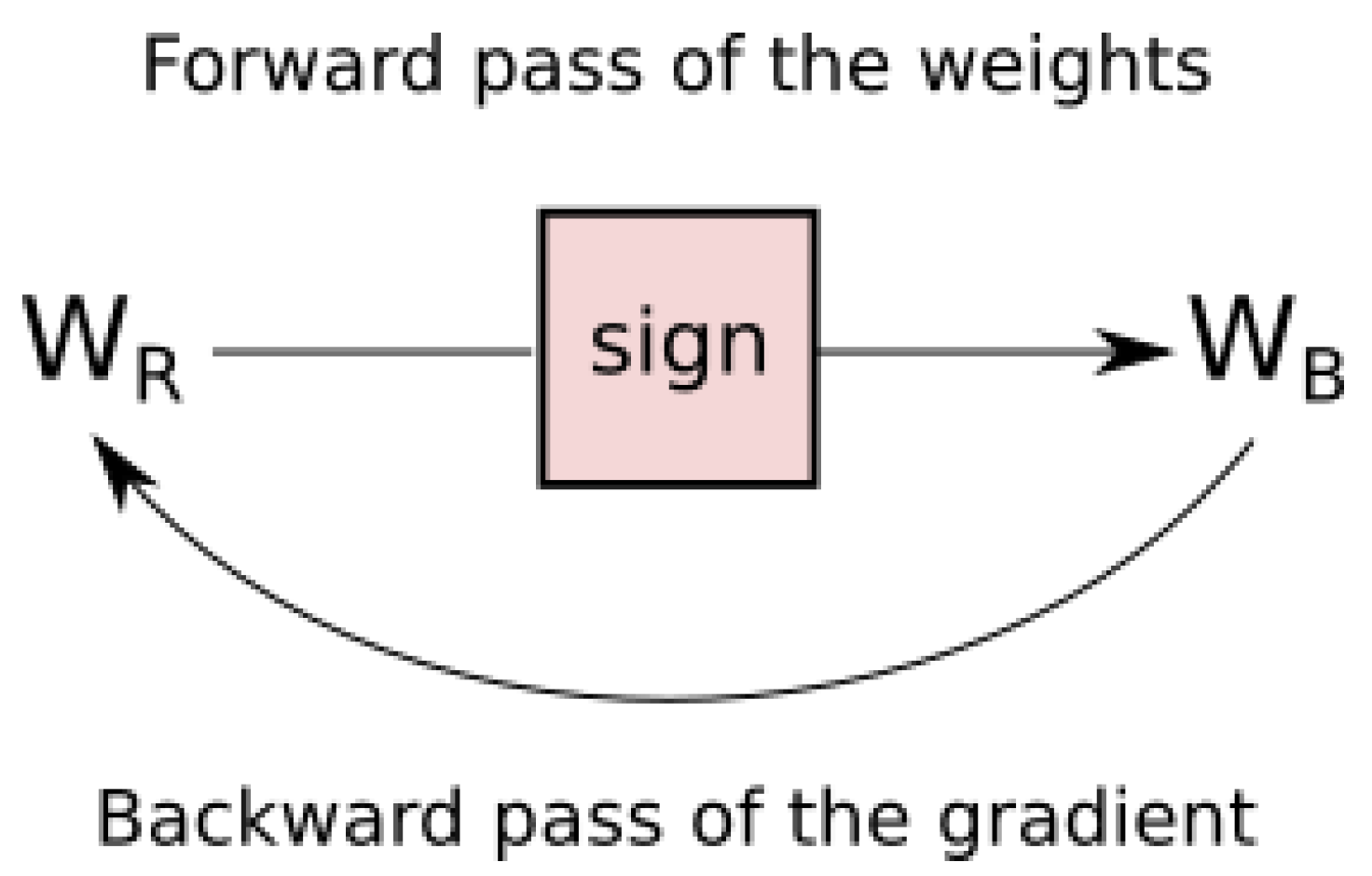
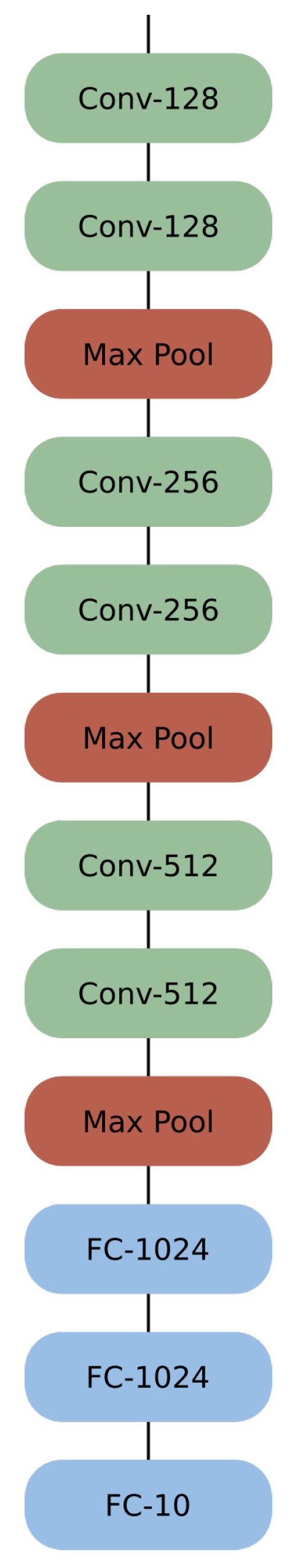
Table 1.
This table shows how the XNOR operation of the endorsing can be equivalent to multiplications of the binary values, in parenthesis.
Table 1.
This table shows how the XNOR operation of the endorsing can be equivalent to multiplications of the binary values, in parenthesis.
| Encoding (Value) | XNOR (Multiply) | |
|---|---|---|
| 0 (−1) | 0 (−1) | 1 (+1) |
| 0 (−1) | 1 (+1) | 0 (−1) |
| 1 (+1) | 0 (−1) | 0 (−1) |
| 1 (+1) | 1 (+1) | 1 (+1) |
Table 2.
Comparison of accuracies on the CIFAR-10 dataset from works presented in this section.
| Methodology | Topology | Accuracy (%) |
|---|---|---|
| Original BNN | BNN | 89.85 |
| XNOR-Net | BNN | 89.83 |
| BNN+ | AlexNet | 87.16 |
| BNN+ | DoReFa-Net | 83.92 |
Table 3.
Comparison of accuracies on the ImageNet dataset from works presented in this section. Full precision network accuracies are included for comparison as well.
Table 3.
Comparison of accuracies on the ImageNet dataset from works presented in this section. Full precision network accuracies are included for comparison as well.
| Methodology | Topology | Top-1 Accuracy (%) | Top-5 Accuracy (%) |
|---|---|---|---|
| Original BNN | AlexNet | 41.8 | 67.1 |
| Original BNN | GoogleNet | 47.1 | 69.1 |
| XNOR-Net | AlexNet | 44.2 | 69.2 |
| XNOR-Net | ResNet18 | 51.2 | 73.2 |
| DoReFa-Net | AlexNet | 43.6 | - |
| Tang et al. | 51.4 | 75.6 | |
| ABC-Net | ResNet18 | 65.0 | 85.9 |
| ABC-Net | ResNet34 | 68.4 | 88.2 |
| ABC-Net | ResNet50 | 76.1 | 92.8 |
| BNN+ | AlexNet | 46.11 | 75.70 |
| BNN+ | ResNet18 | 52.64 | 72.98 |
| Full Precision | AlexNet | 57.1 | 80.2 |
| Full Precision | GoogleNet | 71.3 | 90.0 |
| Full Precision | ResNet18 | 69.3 | 89.2 |
| Full Precision | ResNet34 | 73.3 | 91.3 |
| Full Precision | ResNet50 | 76.1 | 92.8 |
Table 4.
A table of major details of the methods presented in this section. Activation refers to which kind of activation function is used. Gain describes how gain terms were added to the network. Multiplicity refers to how many binary convolutions were performed in parallel in place of full precision convolution layers. The regularization column indicates which kind of regularization was used, if any.
| Methodology | Activation | Gain | Multiplicity | Regularization |
|---|---|---|---|---|
| Original BNN | Sign Function | None | 1 | None |
| XNOR-Net | Sign Function | Statistical | 1 | None |
| DoReFa-Net | Sign Function | Learned Param. | 1 | None |
| Tang et al. | PReLU | Inside PReLU | 2 | L2 |
| ABC-Net | Sign w/Thresh. | Learned Param. | 5 | None |
| BNN+ | Sign w/ for STE | Learned Param. | 1 | L1 and L2 |
Table 5.
BNN accuracies on the MNIST dataset. The accuracy reported for [51] was not explicitly stated by the authors. This number was inferred from the figure provided.
Table 5.
BNN accuracies on the MNIST dataset. The accuracy reported for [51] was not explicitly stated by the authors. This number was inferred from the figure provided.
| Source | Accuracy (%) | Topology |
|---|---|---|
| [52] | 95.7 | FC200-3FC100-FC10 |
| [1] | 96.0 | MLP |
| [51] | 97 | NK |
| [53] | 97.0 | LeNet |
| [54] | 97.69 | MLP |
| [55] | 97.86 | ConvPool-2 |
| [35] | 98.25 | 1/4 MLP |
| [41] | 98.4 | MLP |
| [56] | 98.40 | MLP |
| [57] | 98.6 | NK |
| [58] | 98.67 | MLP |
| [59] | 98.77 | FC784-3FC512-FC10 |
Table 6.
Accuracies on the MNIST dataset of non-binary networks related to works reviewed.
| Source | Accuracy (%) | Topology | Precision |
|---|---|---|---|
| [14] | 95.15 | NK | Ternary values |
| [60] | 96.9 | NK | 8-bit values |
| [60] | 97.2 | NK | 12-bit values |
| [58] | 98.53 | MLP | 2-bits values |
| [19] | 98.71 | BinaryConnect deterministic | 32-bit float activations |
| [54] | 98.74 | MLP | 32-bit float |
| [19] | 98.82 | BinaryConnect stochastic | 32-bit float activations |
| [12] | 99.1 | NK | Ternary values |
Table 7.
BNN accuracies on the SVHN dataset.
| Source | Accuracy | Topology |
|---|---|---|
| [54] | 94.9 | 1/2 BNN |
| [41] | 94.9 | 1/2 BNN |
| [39] | 96.9 | NK |
| [35] | 97.00 | C64-MP-2C128-MP-2C256-2FP512-FP10 |
| [11] | 97.1 | DoReFa-Net |
| [1] | 97.47 | 1/2 BNN |
Table 8.
Accuracies on the SVHN dataset of non-binary networks related to works reviewed.
| Source | Accuracy (%) | Topology | Precision |
|---|---|---|---|
| [15] | 97.60 | 1/2 BNN | Ternary weights |
| [15] | 97.70 | BNN | Ternary weights |
| [19] | 97.70 | BinaryConnect—deterministic | 32-bit float activations |
| [19] | 97.85 | BinaryConnect—stochastic | 32-bit float activations |
Table 9.
BNN accuracies on the CIAFR-10 dataset.
| Source | Accuracy (%) | Topology | Disambiguation |
|---|---|---|---|
| [61] | 66.63 | 2 conv. and 2 FC | |
| [40] | 79.1 | 1/4 BNN | |
| [41] | 80.1 | 1/2 BNN | |
| [54] | 80.1 | 1/2 BNN | |
| [13] | 80.4 | VGG16 | |
| [62] | 81.8 | VGG11 | |
| [57] | 83.27 | NK | |
| [40] | 88.3 | BNN | |
| [34] | 83.52 | DoReFa-Net | R2 regularizer |
| [34] | 83.92 | DoReFa-Net | R1 regularizer |
| [55] | 84.3 | NK | |
| [40] | 85.2 | 1/2 BNN | |
| [63] | 85.9 | 6 conv. | |
| [53] | 86.0 | ResNet-18 | |
| [64] | 86.05 | 9 256-ch conv. | |
| [61] | 86.06 | 5 conv. and 2 FC | |
| [65] | 86.78 | NK | |
| [35] | 86.98 | C64-MP-2C128-MP-2C256-2FC512-FC10 | |
| [51] | 87 | NK | |
| [34] | 87.16 | AlexNet | R1 regularizer |
| [34] | 87.30 | AlexNet | R2 regularizer |
| [38] | 87.73 | BNN | padding |
| [32] | 88 | BNN | 512 channels for FC |
| [38] | 88.42 | BNN | 0 padding |
| [59] | 88.47 | 6 conv. | |
| [39] | 88.61 | NK | |
| [1] | 89.85 | BNN |
Table 10.
Accuracies on the CIFAR-10 dataset of non-binary networks related to works reviewed.
| Source | Accuracy(%) | Topology | Precision |
|---|---|---|---|
| [13] | 81.0 | VGG16 | Ternary values |
| [13] | 82.9 | VGG16 | Ternary values |
| [15] | 86.71 | 1/2 BNN | Ternary values |
| [15] | 89.39 | BNN | Ternary values |
| [19] | 90.10 | BinaryConnect—deterministic | 32-bit float activations |
| [19] | 91.73 | BinaryConnect—stochastic | 32-bit float activations |
Table 11.
BNN accuracies on the ImageNet dataset.
| Source | Top 1 Acc. (%) | Top 5 Acc. (%) | Topology | Details |
|---|---|---|---|---|
| [21] | 36.1 | 60.1 | BNN AlexNet | |
| [11] | 40.1 | Alexnet | ||
| [35] | 41.43 | Details in [35] | ||
| [30] | 41.8 | 67.1 | BNN AlexNet | |
| [31] | 44.2 | 69.2 | AlexNet | |
| [11] | 43.6 | Alexnet | Pre-trained on full precision | |
| [34] | 45.62 | 70.13 | AlexNet | R2 reg |
| [34] | 46.11 | 75.70 | AlexNet | R1 reg |
| [21] | 47.1 | 69.1 | BNN GoogleNet | |
| [36] | 48.2 | 71.9 | AlexNet | Partial binarization |
| [31] | 51.2 | 73.2 | ResNet18 | |
| [34] | 52.64 | 72.98 | ResNet-18 | R1 reg |
| [34] | 53.01 | 72.55 | ResNet-18 | R2 reg |
| [66] | 54.8 | 77.7 | ResNet-18 | Partial binarization |
| [67] | 55.8 | 78.7 | AlexNet | Partial binarization |
| [25] | 65.0 | 85.9 | ResNet-18 | 5 bases |
| [25] | 68.4 | 88.2 | ResNet-34 | 5 bases |
| [25] | 70.1 | 89.7 | ResNet-50 | 5 bases |
| [68] | 75 | VGG 16 | ||
| [33] | 75.6 | 51.4 | AlexNet | binarized last layer |
Table 12.
Comparison of FPGA implementations. The accuracies reported from [68,70] were not explicitly stated. These numbers were inferred from figures provided. The accuracy for [68] is assumed to be a top-5 accuracy and the accuracy for [35] is assumed to top-1 accuracy, but this was never stated by their respective authors. Datasets: MNIST = MN, SVHN = SV, CIFAR-10 = CI, ImageNet = IN.
| Source | Dataset | Acc. (%) | Topology | FPGA | LUTs | BRAMs | Clk (MHz) | FPS | Power (W) |
|---|---|---|---|---|---|---|---|---|---|
| [54] | MN | 97.69 | MLP | Zynq7 020 | 25,358 | 220 | 100 | 2.5 | |
| [54] | MN | 97.69 | MLP | ZynqUltra 3EG | 38,205 | 417 | 300 | 11.8 | |
| [35] | MN | 98.25 | See Table 5 | Spartan7 50 | 32,600 | 120 | 200 | ||
| [41] | MN | 98.4 | MLP | Zynq7 045 | 82,988 | 396 | 1,561,000 | 22.6 | |
| [56] | MN | 98.40 | MLP | Kintex7 325T | 40,000 | 110 | 100 | 10,000 | 12.22 |
| [41] | SV | 94.9 | 1/2 BNN | Zynq7 045 | 46,253 | 186 | 21,900 | 11.7 | |
| [39] | SV | 96.9 | 6 Conv/3 FC | Zynq7 020 | 29,600 | 103 | 6451 | 3.2 | |
| [35] | SV | 97.00 | See Table 7 | Zynq7 020 | 53,200 | 280 | 200 | ||
| [61] | CI | 66.63 | 2 Convs/2 FC | Zynq7 045 | 20,264 | ||||
| [70] | CI | 78 | See Table 9 | Vertex7 690T | 20,352 | 372 | 450 | 15.44 | |
| [40] | CI | 79.1 | 1/4 BNN | KintexUltra 115 | 35,818 | 144 | 125 | 12,000 | |
| [54] | CI | 80.10 | 1/2 BNN | ZynqUltra 3EG | 41,733 | 283 | 300 | 10.7 | |
| [54] | CI | 80.10 | 1/2 BNN | Zynq7 020 | 25,700 | 242 | 100 | 2.25 | |
| [41] | CI | 80.1 | 1/2 BNN | Zynq7 045 | 46,253 | 186 | 21,900 | 11.7 | |
| [62] | CI | 81.8 | 1/2 BNN | Zynq7 020 | 14,509 | 32 | 143 | 420 | 2.3 |
| [40] | CI | 85.2 | 1/2 BNN | KintexUltra 115 | 93,755 | 386 | 125 | 12,000 | |
| [63] | CI | 85.9 | See Table 9 | Zynq7 020 | 23,426 | 135 | 143 | 930 | 2.4 |
| [61] | CI | 86.06 | 5 Convs/2 FC | Vertex7 980T | 556,920 | 340 | 332,158 | ||
| [35] | CI | 86.98 | See Table 9 | Zynq7 020 | 53,200 | 280 | 200 | ||
| [38] | CI | 87.73 | See Table 9 | Zynq7 020 | 46,900 | 140 | 143 | 4.7 | |
| [40] | CI | 88.3 | BNN | KintexUltra 115 | 392,947 | 1814 | 125 | 12,000 | |
| [39] | CI | 88.61 | 6 Conv/3 FC | Zynq7 020 | 29,600 | 103 | 520 | 3.3 | |
| [35] | IN | 41 | See Table 11 | VirtexUltra 095 | 1,075,200 | 3456 | 200 | ||
| [68] | IN | 75 | VGG 116 | ZynqUltra 9EG | 191,784 | 1367 | 150 | 31.48 | 22 |
© 2019 by the authors. Licensee MDPI, Basel, Switzerland. This article is an open access article distributed under the terms and conditions of the Creative Commons Attribution (CC BY) license (http://creativecommons.org/licenses/by/4.0/).
Share and Cite
MDPI and ACS Style
Simons, T.; Lee, D.-J. A Review of Binarized Neural Networks. Electronics 2019, 8, 661. https://doi.org/10.3390/electronics8060661
AMA Style
Simons T, Lee D-J. A Review of Binarized Neural Networks. Electronics. 2019; 8(6):661. https://doi.org/10.3390/electronics8060661
Chicago/Turabian StyleSimons, Taylor, and Dah-Jye Lee. 2019. "A Review of Binarized Neural Networks" Electronics 8, no. 6: 661. https://doi.org/10.3390/electronics8060661
Note that from the first issue of 2016, this journal uses article numbers instead of page numbers. See further details here.