Features Dimensionality Reduction Approaches for Machine Learning Based Network Intrusion Detection

Abstract

The security of networked systems has become a critical universal issue that influences individuals, enterprises and governments. The rate of attacks against networked systems has increased dramatically, and the tactics used by the attackers are continuing to evolve. Intrusion detection is one of the solutions against these attacks. A common and effective approach for designing Intrusion Detection Systems (IDS) is Machine Learning. The performance of an IDS is significantly improved when the features are more discriminative and representative. This study uses two feature dimensionality reduction approaches: (i) Auto-Encoder (AE): an instance of deep learning, for dimensionality reduction, and (ii) Principle Component Analysis (PCA). The resulting low-dimensional features from both techniques are then used to build various classifiers such as Random Forest (RF), Bayesian Network, Linear Discriminant Analysis (LDA) and Quadratic Discriminant Analysis (QDA) for designing an IDS. The experimental findings with low-dimensional features in binary and multi-class classification show better performance in terms of Detection Rate (DR), F-Measure, False Alarm Rate (FAR), and Accuracy. This research effort is able to reduce the CICIDS2017 dataset’s feature dimensions from 81 to 10, while maintaining a high accuracy of 99.6% in multi-class and binary classification. Furthermore, in this paper, we propose a Multi-Class Combined performance metric $Combine{d}_{Mc}$ with respect to class distribution to compare various multi-class and binary classification systems through incorporating FAR, DR, Accuracy, and class distribution parameters. In addition, we developed a uniform distribution based balancing approach to handle the imbalanced distribution of the minority class instances in the CICIDS2017 network intrusion dataset.

1. Introduction

Network Intrusion Detection System (IDS) is a software-based application or a hardware device that is used to identify malicious behavior in the network [1,2]. Based on the detection technique, intrusion detection is classified into anomaly-based and signature-based. IDS developers employ various techniques for intrusion detection. One of these techniques is based on machine learning. Machine learning (ML) techniques can predict and detect threats before they result in major security incidents [3]. Classifying instances into two classes is called binary classification. On the other hand, multi-class classification refers to classifying instances into three or more classes. In this research, we adopt both classifications. For the multi-class classification, there are 15 classes, where each class represents either normal network flow traffic or one of 14 types of attacks. For the binary case, the network flow traffic is being classified into either normal or anomaly (attack) traffic.

An Artificial Neural Network (ANN) is a self-adaptive mathematical and computational model that is composed of an interconnected group of artificial neurons. There are multiple types of ANNs such as Deep Convolution Neural Networks (DCNN), Recurrent Neural Networks (RNN) and Auto-Encoder (AE) neural networks, each of which come with their own specific applications and levels of complexity. Deep learning is a promising machine learning-based approach that can address the challenges associated with the design of intrusion detection systems as a result of its outstanding performance in dealing with complex, large-scale data.

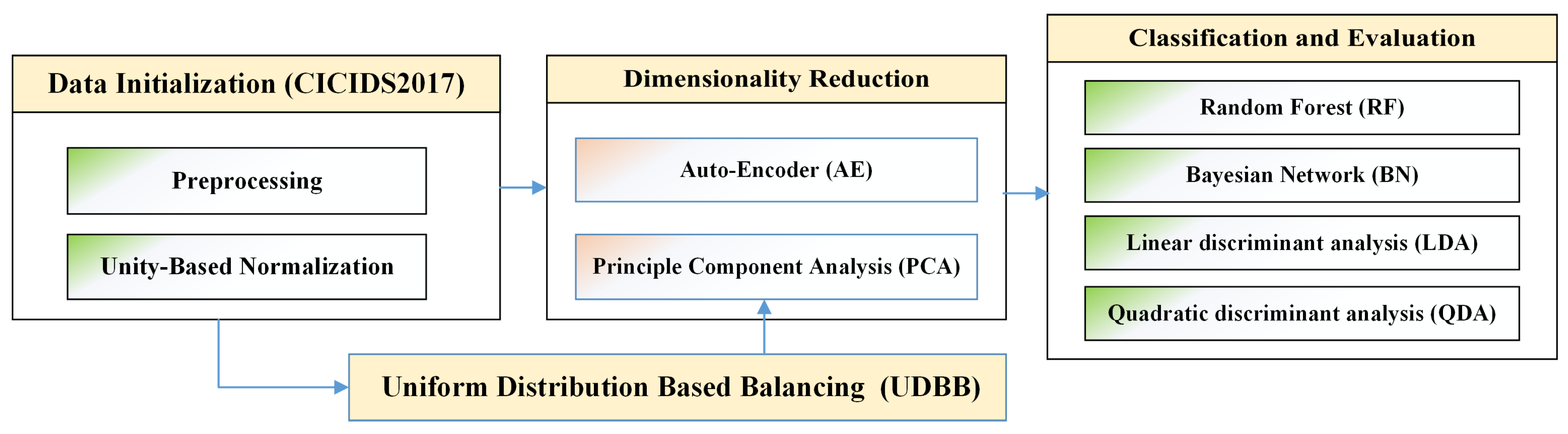
This study accustoms Auto-Encoder (AE) and Principle Component Analysis (PCA) for dimensionality reduction. As a proof-of-concept and to verify the feature dimensionality reduction ideas, the paper used the up-to-date CICIDS2017 intrusion detection and prevention dataset [4], which consists of five separated data files. Each file represents the network traffic flow and specific types of attacks for a certain period of time. To be more specific, the dataset was collected based on a total of 5 days, Monday through Friday. The traffic flow on Monday includes the benign network traffic, whereas the implemented attacks in the dataset were executed on Tuesday, Wednesday, Thursday and Friday. In this paper, we combined all CICIDS2017’s files together and fed them through the AE and PCA units for a compressed and lower dimensional representation of all the fused data. Figure 1 displays the overall idea of the proposed framework.

1.1. Problem Statement

In machine learning problems, the high-dimensional features lead to prolonged classification processes. This is while low-dimensional features can reduce these processes. Moreover, classification of network traffic data with imbalanced class distributions has posed a significant drawback on the performance attainable by most well-known classifiers, which assume relatively balanced class distributions and equal miss-classification costs. The frequent occurrence and issues associated with imbalanced class distributions indicate the need for extra research efforts. Previous studies of intrusion detection systems have not dealt with classification of network traffic data with imbalanced class distributions. Furthermore, with the presence of imbalanced data, the known performance metrics may fail to provide adequate information about the performance of the classifier.

1.2. Key Contributions and Paper Organization

The key contributions of this paper include the development of a framework for machine learning-based network intrusion detection. The proposed anomaly-based intrusion detection system uses AE as well as PCA for dimensionality reduction and well-tested classifiers such as Random Forest (RF), Bayesian Network (BN), Linear Discriminant Analysis (LDA) and Quadratic Discriminant Analysis (QDA). In summary, the main contributions of this work are as follows:

• We achieved effective pattern representation and dimensionality reduction of features in the CICIDS2017 dataset using AE and PCA.
• We used the CICIDS2017 dataset to compare the efficiency of the dimensionality reduction approaches with different classification algorithms, such as Random Forest, Bayesian Network, LDA and QDA in binary and multi-class classification.
• We developed a combined metric with respect to class distribution to compare various multi-class classification systems through incorporating the False Alarm Rate (FAR), Detection Rate (DR), Accuracy and class distribution parameters.
• We developed a Uniform Distribution Based Balancing (UDBB) approach for imbalanced classes.

The overall structure of the remainder of this paper is organized as follows. An overview of the dimensionality reduction approaches selection criteria and related work is provided in Section 2. Next, in Section 3, the paper gives a brief review of the CICIDS2017 dataset, describes the attack types embedded in the dataset, and further explains the preprocessing and unity-based normalization steps. In Section 4, the paper explains in detail, the dimensionality reduction approaches based on AE as well as PCA. Afterwards, the performance evaluation metrics are introduced in Section 5. Section 6 elaborates on the Uniform Distribution Based Balancing (UDBB) approach. Next, in Section 7, the paper summarizes the principal findings of the experiments and discusses the results. The challenges and limitations are discussed in Section 8. Finally, the conclusions and future directions are discussed in Section 9.

2. Dimensionality Reduction Approaches Selection Criteria and Related Work

This section aims to review the published related work in the past recent years that used features dimensionality reduction approaches to design an intrusion detection system. The selection process was based on certain criteria such as:

• Being relevant to the CICIDS2017 dataset
• Being relevant to dimensionality reduction approaches; precisely, the auto-encoder and the PCA
• Being relevant to machine learning-based intrusion detection

For decades, researchers used dimensionality reduction approaches [5,6] for different reasons such as to reduce the computational processing overhead, reduce noise in the data, and for better data visualization and interpretation. One common dimensionality reduction approach is the Missing Value Ratio (MVR) approach [7]. The MVR approach is efficient when the number of missing values is high. For the CICIDS2017 dataset, the number of missing values is near zero. Therefore, we excluded the Missing Value Ratio approach. Other common approaches include the Forward Feature Construction (FFC) and Backward Feature Elimination (BFE) approaches [7]. Both FFC and BFE are prohibitively slow on high dimensional datasets, which is the case for CICIDS2017 (>2,500,500 instances). As a result, we did not discuss these approaches. The PCA technique, on the other hand, is relatively computationally cost efficient, can deal with large datasets, and is widely used as a linear dimensionality reduction approach [5,8]. The auto-encoder dimensionality reduction approach is an instance of deep learning, which is also suitable for large datasets with high dimensional features and complex data representations [9].

This paper adopts AE as well as PCA for features dimensionality reduction. One of the most fundamental differences between AE and PCA in terms of dimensionality reduction is that in the auto-encoder approach, there is no assumption of linearity in the data. The auto-encoder optimizer figures out the function through the weights that best encode the data under the specified reconstruction error metric. This is while the PCA assumes linearity in the set of reduced data. Moreover, the computational complexity of a dimensionality reduction approach depends on the number of datapoints n as well as their dimensionality P, and w which is the number of weights in the auto-encoder.

Table 1. Properties of analyzed approaches for dimensionality reduction [8,9].

Technique	Computational	Memory	Pros	Cons
	Complexity	Complexity
PCA	$O(P^3)$	$O(P^2)$	Can deal with large datasets; fast run time	Hard to model nonlinear structures
AE	$O(n^2)$	$O(w)$	Can model linear and nonlinear structures	Slow run time; prone to overfitting

shows the properties of AE and PCA for dimensionality reduction and lists the pros and cons of each.

2.1. CICIDS2017 Related Work

Sharafaldin et al. [4] used a Random Forest Regressor to determine the best set of features to detect each attack family. The authors examined the performance of these features with different algorithms that included K-Nearest Neighbor (KNN), Adaboost, Multi-Layer Perceptron (MLP), Naïve Bayes, Random Forest (RF), Iterative Dichotomiser 3 (ID3) and Quadratic Discriminant Analysis (QDA). The highest precision value was 0.98 with RF and ID3 [4]. The execution time (time to build the model) was 74.39 s. This is while the execution time for our proposed system using Random Forest is 21.52 s with a comparable processor. Furthermore, our proposed intrusion detection system targets a combined detection process of all the attack families.

In wireless mesh environments, Vijayan et al. [10] proposed an intrusion detection system that used the genetic algorithm (GA) as a feature selection method and multiple Support Vector Machines (SVM) for classification. Their system was based on a linear combination of multiple SVM classifiers, which were ordered based on the severity of the attacks. Each classifier was trained to detect a certain attack category using selected features by the GA. A small portion of the CICIDS2017 dataset instances were used to evaluate their system. Conversely, in this paper, we use all the instances of the CICIDS2017 dataset.

Moreover, authors in [11] compared and contrasted a frequency-based model from five sequence of aggregation rules with sequence-based modeling of the Long Short-Term Memory (LSTM) recurrent neural network. The investigation concluded that the frequency-based model tends to perform similar or better than the LSTM models in detecting the attacks.

Additionally, the researchers in [12] analyzed the CICIDS2017 dataset using digital wavelets. Their method efficiently detected service denial attacks of both Slow Loris and HTTP Denial of Service (DoS).

Furthermore, the authors of [13] applied the Multi-Layer Perceptron (MLP) classifier algorithm and a Convolutional Neural Network (CNN) classifier that used the Packet CAPture (PCAP) file of CICIDS2017. The authors selected specified network packet header features for the purpose of their study. Conversely, in our paper, we used the corresponding profiles and the labeled flows for machine and deep learning purposes. According to [13], the results demonstrated that the payload classification algorithm was judged to be inferior to MLP. However, it showed significant ability to distinguish network intrusion from benign traffic with an average true positive rate of 94.5% and an average false positive rate of 4.68%.

The authors in [14] proposed a denial of service intrusion detection system that used the Fisher Score algorithm for features selection and Support Vector Machine (SVM), K-Nearest Neighbor (KNN) and Decision Tree (DT) as the classification algorithm. Their IDS achieved 99.7%, 57.76% and 99% success rates using SVM, KNN and DT, respectively. In contrast, our research proposes an IDS to detect all types of attacks embedded in CICIDS2017, and as shown in the confusion matrix results, achieves 100% accuracy for DDoS attacks using (${PCA-RF)}_{Mc-10}$ with UDBB.

The authors in [15] used a distributed Deep Belief Network (DBN) as the the dimensionality reduction approach. The obtained features were then fed to a multi-layer ensemble SVM. The ensemble SVM was accomplished in an iterative reduce paradigm based on Spark (which is a general distributed in-memory computing framework developed at AMP Lab, UC Berkeley), to serve as a Real Time Cluster Computing Framework that can be used in big data analysis [16]. Their proposed approach achieved an F-measure value equal to 0.921.

The authors in [17] proposed a Data Dimensionality Reduction (DDR) method for network intrusion detection. Their proposed scheme was evaluated by XGBoost (Extreme Gradient Boosting) [18], SVM (Support Vector Machine), CTree (Conditional inference Trees) [19] and Neural network (Nnet) classifiers. The number of selected features was 36 and the highest achieved accuracy was 98.93% with XGboost. Furthermore, the authors excluded Monday network traffic of the CICIDS2017 dataset, which is only benign traffic in their system. This is while our work was able to achieve accuracy of 99.6% with 10 features. In addition, we kept all the files of the dataset that represent different classes of the network traffic.

2.2. Auto-Encoder Related Work

Regarding using Auto-Encoder for dimensionality reduction, authors in [20] proposed a framework for IDS using a Stacked Auto Encoder (SAE), which is an unsupervised learning method for attribute selection. Their framework used regression layer, a supervised learning technique, with SoftMax activation function for the classification process.

The authors in [21] developed an intrusion detection system for wireless sensor networks using Deep Auto-Encoder (DAE) as the basic classifier to the detect attack type. The authors used a cross-entropy loss function and back-propagation algorithm in an attempt to prevail over the slow update of the weights in the case of traditional varying cost functions with exponential costs [21].

The authors in [22] used Sparse Auto-Encoder (SAE) for feature learning and dimensionality reduction on the NSL-KDD dataset [23], which is an enhanced version of KDD-CUP99 [24]; an old, outdated synthetic netflow dataset. The authors used Support Vector Machines (SVM) and achieved an accuracy of 84.96% in binary classification and 99.39% in multi-class classification of five classes. In our work, we used CICIDS2017, which is an up-to-date dataset that accommodates new attacks and intruder strategies. Moreover, the total instances of the NSL-KDD is 125,923 in training and 22,544 instances in testing. This is while CICIDS2017 has 2,830,108 instances and is generated based on real network traffic.

In the same manner, ref. [25] proposed a system based on the same methodology of [22]. The authors in [25] used SAE with SVM on the NSL-KDD dataset. The framework of [25] achieved 88.39% accuracy in binary classification and 79.10% in five class classification.

The authors in [26] proposed SU-IDS; a semi-supervised and unsupervised network intrusion detection system that used an auto-encoder-based framework. The framework augments the usual clustering (or classification) loss with an auxiliary loss of auto-encoder, and thus achieves a better performance. A comparison between the experimental results of the classic NSL-KDD dataset and the modern CICIDS2017 dataset show the superiority of our proposed models.

2.3. PCA Related Work

The authors in [27] implemented an IDS that used Principal Component Analysis (PCA) as the feature reduction approach and Grey Neural Networks (GNN) as the classifier on the KDD-99 dataset.

In the same context, ref. [27] used PCA for features reduction and decision tree and Nearest Neighbor as classifiers on KDD-99.

The researchers in [28] defined the reduction rate and studied the efficiency of PCA for intrusion detection. The authors fulfilled their experiments using Random Forest and C4.5 on KDD-CUP [24] and UNB-ISCX [29].

3. CICIDS2017 Dataset

The CICIDS2017 dataset consists of realistic background traffic that represents the network events produced by the abstract behavior of a total of 25 users. The users’ profiles were determined to include specific protocols such as HTTP, HTTPS, FTP, SSH and email protocols. The developers used statistical metrics such as minimum, maximum, mean and standard deviation to encapsulate the network events into a set of certain features which include:

• The distribution of the packet size
• The number of packets per flow
• The size of the payload
• The request time distribution of the protocols
• Certain patterns in the payload

Moreover, CICIDS2017 covers various attack scenarios that represent common attack families. The attacks include Brute Force Attack, HeartBleed Attack, Botnet, DoS Attack, Distributed DoS (DDoS) Attack, Web Attack, and Infiltration Attack.

The dataset is publicly available by the authors in two formats:

• The full packet payloads in Packet CAPture (PCAP) format
• The corresponding profiles and labeled flows as CSV files for machine and deep learning purposes

CICIDS2017 was collected based on real traces of benign and malicious activities of the network traffic. The total number of records in the dataset is 2,830,108. The benign traffic encompasses 2,358,036 records (83.3% of the data), while the malicious records are 471,454 (16.7% of the data). CICIDS2017 is one of the unique datasets that includes up-to-date attacks. Furthermore, the features are exclusive and matchless in comparison with other datasets such as UNSW-NB15 [30,31], AWID [32], GPRS [33], and CIDD-001 [34]. For this reason, CICIDS2017 was selected as the most comprehensive IDS benchmark to test and validate the proposed ideas.

Table 2. CICIDS2017 attack distribution and description.

Traffic Type	Size	Description
Benign	2,358,036	Normal traffic behavior
DoS Hulk	231,073	The attacker employs the HULK tool to carry out a denial of service attack on a web server through generating
		volumes of unique and obfuscated traffic. Moreover, the generated traffic can bypass caching engines and strike
		a server’s direct resource pool
Port Scan	158,930	The attacker tries to gather information related to the victim machine such as type of operating system
		and running service by sending packets with varying destination ports
DDoS	41,835	The attacker uses multiple machines that operate together to attack one victim machine
DoS GoldenEye	10,293	The attacker uses the GoldenEye tool to perform a denial of service attack
FTP Patator	7938	The attacker uses FTP Patator in an attempt to perform a brute force attack to guess the FTP login password
SSH Patator	5897	The attacker uses SSH Patator in an attempt to perform a brute force attack to guess the SSH login Password
DoS Slow Loris	5796	The attacker uses the Slow Loris tool to execute a denial of service attack
DoS Slow HTTP Test	5499	The attacker exploits the HTTP Get request to exceed the number of HTTP connections allowed on
		a server, preventing other clients from accessing and giving the attacker the opportunity to open multiple
		HTTP connections to the same server
Botnet	1966	The attacker uses trojans to breach the security of several victim machines, taking control of these machines
		and organizes all machines in the network of Bot that can be exploited and managed remotely by the attacker
Web Attack: Brute Force	1507	The attacker tries to obtain privilege information such as password and Personal Identification Number (PIN)
		using trial-and-error
Web Attack: XSS	625	The attacker injects into otherwise benign and trusted websites using a web application that sends malicious scripts
Infiltration	36	The attacker uses infiltration methods and tools to infiltrate and gain full unauthorized access to the networked
		system data
Web Attack: SQL Injection	21	SQL injection is a code injection technique, used to attack data-driven applications,
		in which nefarious SQL statements are inserted into an entry field for execution
HeartBleed	11	The attacker exploits the OpenSSL protocol to insert malicious information into OpenSSL memory,
		enabling the attacker with unauthorized access to valuable information

highlights the characteristics and distribution of the attacks in the CICIDS2017 dataset and provides a brief description of each type of attack. CICIDS2017 is a labeled dataset with a total number of 84 features including the last column corresponding to the traffic status (class label). The features were extracted by CICFlowMeter-V3 [35]. The output of CICFlowMeter-V3 is a CSV file that includes: Flow ID (1), Source IP (2) and Destination IP (4), Time stamp (7) and Label (84). The Flow ID (1) includes the four tuples: Source IP, Source Port, Destination IP, and Destination Port. Time stamp represents the timing. To the best of our knowledge, all previous studies that used CICIDS2017 neglect Flow ID (1), Source IP (2), Destination IP (4), and Time stamp (7). In this paper, we used CICIDS2017 with respect to the listed features except the Flow ID (1) and Time Stamp (7). Thus, in our study, the total number of used features encompasses 82 features including the Label (84). These features are listed in

Table 3. Listed features of network traffic in CICIDS2017.

No.	Feature	No.	Feature	No.	Feature
1	Flow ID	29	Fwd IAT Std	57	ECE Flag Count
2	Source IP	30	Fwd IAT Max	58	Down/Up Ratio
3	Source Port	31	Fwd IAT Min	59	Average Packet Size
4	Destination IP	32	Bwd IAT Total	60	Avg Fwd Segment Size
5	Destination Port	33	Bwd IAT Mean	61	Avg Bwd Segment Size
6	Protocol	34	Bwd IAT Std	62	Fwd Avg Bytes/Bulk
7	Time stamp	35	Bwd IAT Max	63	Fwd Avg Packets/Bulk
8	Flow Duration	36	Bwd IAT Min	64	Fwd Avg Bulk Rate
9	Total Fwd Packets	37	Fwd PSH Flags	65	Bwd Avg Bytes/Bulk
10	Total Backward Packets	38	Bwd PSH Flags	66	Bwd Avg Packets/Bulk
11	Total Length of Fwd Pck	39	Fwd URG Flags	67	Bwd Avg Bulk Rate
12	Total Length of Bwd Pck	40	Bwd URG Flags	68	Subflow Fwd Packets
13	Fwd Packet Length Max	41	Fwd Header Length	69	Subflow Fwd Bytes
14	Fwd Packet Length Min	42	Bwd Header Length	70	Subflow Bwd Packets
15	Fwd Pck Length Mean	43	Fwd Packets/s	71	Subflow Bwd Bytes
16	Fwd Packet Length Std	44	Bwd Packets/s	72	Init_Win_bytes_fwd
17	Bwd Packet Length Max	45	Min Packet Length	73	Act_data_pkt_fwd
18	Bwd Packet Length Min	46	Max Packet Length	74	Min_seg_size_fwd
19	Bwd Packet Length Mean	47	Packet Length Mean	75	Active Mean
20	Bwd Packet Length Std	48	Packet Length Std	76	Active Std
21	Flow Bytes/s	49	Packet Len. Variance	77	Active Max
22	Flow Packets/s	50	FIN Flag Count	78	Active Min
23	Flow IAT Mean	51	SYN Flag Count	79	Idle Mean
24	Flow IAT Std	52	RST Flag Count	80	Idle Packet
25	Flow IAT Max	53	PSH Flag Count	81	Idle Std
26	Flow IAT Min	54	ACK Flag Count	82	Idle Max
27	Fwd IAT Total	55	URG Flag Count	83	Idle Min
28	Fwd IAT Mean	56	CWE Flag Count	84	Label

. The extracted traffic features are explained in [36].

3.1. Preprocessing

In this study, a preprocessing function is applied to the CICIDS2017 dataset by mapping the IP (Internet Protocol) address to an integer representation. The mapped IP includes the Source IP Address (Src IP) as well as the Destination IP Address (Dst IP). These two are converted to an integer number representation. This study splits the data into training set and testing set with a ratio of 70:30.

3.2. Unity-Based Normalization

In this step, we use Equation (1) to re-scale the features in the dataset based on the minimum and maximum values of each feature. Some features in the original dataset vary between [0, 1] while other features vary between [0, ∞). Therefore, these features are normalized to restrict the range of the values between 0 and 1, which are then processed by the auto-encoder for feature reduction.

$$x_i=\frac{x_i-x_{min}}{x_{max}-x_{min}}$$

(1)

where $x_i$ is the value of a particular feature, $x_{min}$ is the minimum value, and $x_{max}$ is the maximum value.

4. Features Dimensionality Reduction

4.1. Auto-Encoder (AE) Based Dimensionality Reduction

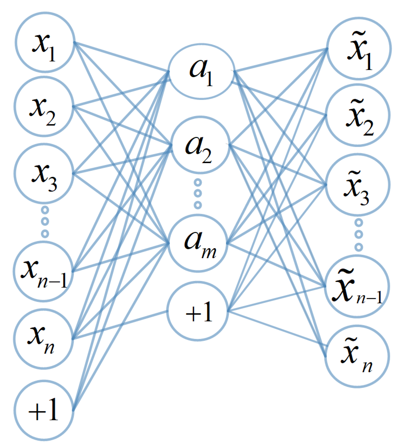
In this section, we present the sparse auto-encoder learning algorithm [37,38], which is one approach to automatically learn feature reduction in unsupervised settings. Figure 2 shows the structure of the auto-encoder. The input vector $x=(x_1,x_2,\dots ,x_n)$ is first compressed to a lower dimensional hidden representation that consists of one or more hidden layers $a=(a_1,a_2,\dots ,a_m)$. The hidden representation a is then mapped to reproduce the output $\widehat{x}=(\widehat{x_1},\widehat{x_2},\dots ,\widehat{x_n})$. Let j be the counter parameter for the neurons in the current layer l, and i be the counter parameter for the neurons in the previous hidden layer $l-1$. The output of a neuron in the hidden layer can be represented by the following formula.

$$a_j^{(l)}=f(z_j^{(l)})=f(\sum _{i=1}^n{W}_{ji}^{(l-1)}.a_i^{(l-1)}+b_j^{(l-1)})$$

(2)

The size of the weight matrix of the hidden layer is represented by $W\in R^{m\times n}$ and the bias is $b\in R^m$. A sigmoid function is chosen as the activation function, such that $f(z)=\frac{1}{(1+ex{p}^{-z})}$. Parameters W and b are optimized using back propagation, by minimizing the cost function J for all the training instances [39], as follows:

$$J(W,b;\widehat{x},x)=\frac{1}{k}\sum _{i=1}^k(\frac{1}{2}\left|\right|\widehat{x}-{x\left|\right|}^2)+\frac{1}{\lambda }\sum _{l=1}^{ls-1}\sum _{j=1}^m\sum _{i=1}^n{(W_{ji}^{(l)})}^2$$

(3)

Parameter $\lambda$ is chosen to control the regularization term of all the weights in a particular layer, and $ls$ denotes the total number of layers. To impose a sparsity constraint on the hidden units, one strategy is to add an additional term in the loss function during training to penalize the Kullback-Leibler (KL) divergence between a Bernoulli random variable with mean $\rho$ and a desired sparsity mean $\widehat{{\rho }_j}$.

$$\widehat{{\rho }_j}=\frac{1}{k}\sum _{i=1}^k\left[a_j^{(i)}(x^{(i)})\right]$$

(4)

where $a_j^{(i)}$ denotes the activation of hidden unit j in the auto-encoder and k is the training sample [40].

$$J{}_{sparse}\left(W,b\right)=J(W,b;\widehat{x},x)+\beta \sum _{j=1}^{m}KL\left(\rho \left|\right|\widehat{{\rho }_j}\right)$$

(5)

This sparsity is guaranteed to have the effect of causing $\widehat{{\rho }_j}$ to be close to $\rho$, because it ensures that the sparse activations are achieved on the training data for any given units in the hidden layer. The value of $\beta$ is chosen to control the weight of the sparsity penalty term.

The computational complexity of executing the designed auto-encoder with a single hidden layer depends on the dimensionality of the input vector n, and the Reduction ratio $R\in (0,1)$ [41].

$$O(n.(R\times n)+(R\times n).n)=O(R{n}^2+R{n}^2)=O(n^2)$$

(6)

In this paper, a two hidden-layer sparse auto-encoder is used with sigmoid activation functions and tied weights. The input layer has 81 neurons which equals the total number of features in the CICIDS2017 dataset. The first hidden layer of the sparse auto-encoder was able to successfully reduce the dimensions to 70 features with a good error approximation. Further, the features were reduced to 64 in the second hidden layer. Once the weights are trained, the resulting sparse auto-encoder can be used to perform the classification in the final stage. The parameters of the sparse representation are set as follows: the weight decay $\lambda =0.0008$. The weights are multiplied by $\lambda$ to prevent the weights from growing too large. The sparsity parameter $\rho =0.05$, and the sparsity penalty term $\beta =6$. The sparsity parameters and penalty are designed to restrict the activation of the hidden units, which reduces the dependency between the features. The algorithm is summarized in

Table 4. Pseudo-code for the proposed Auto-Encoder.

Dimensionality Reduction Using AE
Training:
1. Perform the feedforward pass on all the training
instances and compute
$a^{(1)},a^{(2)}$ Equation (2)
2. Compute the output, sparsity mean,
and the error of the cost function
$J(W,b;\widehat{x},x)$ Equation (3)
$\widehat{{\rho }_j}$ Equation (4)
3. Compute the cost function of the sparse auto-encoder
$J_{sparse}(W,b)$ Equation (5)
4. Backpropagate the error to update the weights and
the bias for all the layers
Dimensionality Reduction:
Compute the reduced features from the hidden layer
$a^{(1)}$        Equation (2)

and the design principles are presented in

Table 5. Design Principles.

Parameters	Value	Description
$\lambda$	0.0008	Weight decay
$\beta$	6	Sparsity penalty
$\rho$	0.05	Sparsity parameter

.

4.2. Principle Component Analysis (PCA) Based Dimensionality Reduction

In this section, we present the Principle Component Analysis (PCA) algorithm. The objective of PCA is to perform dimensionality reduction. PCA finds a transformation that reduces the dimensionality of the data while accounting for as much variance as possible. PCA is the oldest technique in multivariate analysis. The fundamental concept of the PCA is the projection-based mechanism. Here, the original dataset $X\in R^n$ with n columns (features) is projected into a subspace with k or lower dimensions representation $X\in R^K$ (fewer columns), while retaining the essence of the original data. The algorithm works as follows:

To reduce the features dimensionality from n-dimensions to k-dimensions, two phases are implemented; the preprocessing phase and the dimensionality reduction phase. In the preprocessing phase, (steps 1 through 4 below), the data is preprocessed to normalize its mean and variance using Equations (7) and (8). In the second phase (steps 5 through 8), which represent the reduction phase, the covariance matrix $Co{v}_M$, Eigen-vectors and Eigen-values are calculated from Equations (9) and (10).

• Normalize the the original feature values of data by its mean and variance using Equation (7), where m is the number of instances in the dataset and $X_{(i)}$ are the data points.

  $$\mu =\frac{1}{m}\sum _{i=1}^m{X}_{(i)}$$

  (7)
• Replace $X_{(i)}$ with $X_{(i)}-\mu$.
• Rescale each vector $X_{j(i)}$ to have unit variance using Equation (8).

  $${\sigma }_j^2=\frac{1}{m}\sum _i{(X_{j(i)})}^2$$

  (8)
• Replace each $X_{j(i)}$ with $\frac{X_{j(i)}}{\sigma }$.
• Compute the Covariance Matrix $Co{v}_M$ as follows:

  $$Co{v}_M=\frac{1}{m}\sum (X_{(i)}){(X_{(i)})}^{\top }$$

  (9)
• Calculate the Eigen-vectors and corresponding Eigen-values of $Co{v}_M$.
• Sort the Eigen-vectors by decreasing the Eigen-values and choose k Eigen-vectors with the largest Eigen-values to form W.
• Use W to transform the samples onto the new subspace using Equation (10).

  $$y=W^T\times X$$

  (10)

  where X is a $d\times 1$ dimensional vector representing one sample, and y is the transformed $k\times 1$ dimensional sample in the new subspace.

The computational complexity of executing the designed PCA depends on the number of features P that represent each data point [42].

$$O(P^3)$$

(11)

According to [28], the Reduction Ratio (RR) of PCA can be defined as the ratio of the number of target dimensions to the number of original dimensions. The lower the value of RR, the higher is the efficiency of PCA. The RR of our proposed framework is equal to 10:81 which outperformed previous related work. Our final RR of 2:81 is also able to represent the data with low error and provide high accuracies.

5. Performance Evaluation Metrics

This study used various performance metrics to evaluate the performance of the proposed system, including False Alarm Rate (FAR), F-Measure [43], Detection Rate (DR), and Accuracy (Acc) as well as the processing time. The definitions of these metrics are provided below. The metrics are a function of True Positives (TP), True Negatives (TN), False Positives (FP) and False Negatives (FN).

(1)

False Alarm Rate (FAR) is a common term which encompasses the number of normal instances incorrectly classified by the classifier as an attack, and can be estimated through Equation (12).

$$FAR=\frac{FP}{TN+FP}$$

(12)

(2)

Accuracy (Acc) is defined as the ability measure of the classifier to correctly classify an object as either normal or attack. The Accuracy can be defined using Equation (13).

$$Acc=\frac{TP+TN}{TP+TN+FP+FN}$$

(13)

(3)

Detection Rate (DR) indicates the number of attacks detected divided by the total number of attack instances in the dataset. DR can be estimated by Equation (14).

$$DR=\frac{TP}{TP+FN}$$

(14)

(4)

The F-measure (F-M) is a score of a classifier’s accuracy and is defined as the weighted harmonic mean of the Precision and Recall measures of the classifier. F-Measure is calculated using Equation (15).

$$F-Measure=2\times \frac{Precision\times Recall}{Precision+Recall}$$

(15)

(5)

Precision represents the number of positive predictions divided by the total number of positive class values predicted. It is considered as a measure for the classifier exactness. A low value indicates large number of False Positives. The precision is calculated using Equation (16).

$$Precision=\frac{TP}{TP+FP}$$

(16)

(6)

Recall is the number of True Positives divided by the number of True Positives and the number of False Negatives. Recall is considered as a measure of a classifier completeness such that a low value of recall realizes many False Negatives [44]. Recall is estimated through Equation (17).

$$Recall=\frac{TP}{TP+FN}$$

(17)

Proposed Multi-Class Combined Performance Metric with Respect to Class Distribution

In general, the overall accuracy is used to measure the effectiveness of a classifier. Unfortunately, in presence of imbalanced data, this metric may fail to provide adequate information about the performance of the classifier. Furthermore, the method is very sensitive to the class distribution and might be misleading in some way. Hamed et al. [45] proposed a combined performance metric to compare various binary classifier systems. However, their solution neglects class distribution and can work only for binary classifications.

In this paper, we propose the multi-class combined performance metric $Combine{d}_{Mc}$ with respect to class distribution to compare various multi-class classification systems as well as binary class systems through incorporating four metrics together (FAR Equation (12), Accuracy Equation (13), Detection Rate Equation (14), and class distribution Equation (19). The multi-class Combined performance metric can be estimated using the following equation.

$$Combine{d}_{Mc}=\sum _{i=1}^C{\lambda }_i\left(\frac{Ac{c}_i+D{R}_i}{2}-FA{R}_i\right)$$

(18)

where C is number of classes, and ${\lambda }_i$ is the class distribution ($dist$), which can be estimated using the following formula.

$$dist={\lambda }_i=\frac{Numberofinstancesinclassi}{Numberofinstancesinthedataset}$$

(19)

The result of this metric will be a real value between −1 and 1; that is $Combine{d}_{Mc}$ $\in [-1,+1]$; where $-1$ corresponds to the worst overall system performance and 1 corresponds to the best overall system performance.

Table 6. Pseudo-code for the proposed $Combine{d}_{Mc}$ metric calculation.

Calculate ${\mathit{Combined}}_{\mathit{Mc}}$ with respect to Class Distribution
Feed Confusion Matrix CM
For i =1 to C
Calculate the total number of FP for $C_i$ as the sum of values in the $i^{th}$ column excluding TP
Calculate the total number of FN for $C_i$ as the sum of values in the $i^{th}$ row excluding TP
Calculate the total number of TN for $C_i$ as the sum of all columns and rows excluding the $i^{th}$ row and column
Calculate the total number of TP for $C_i$ as the diagonal of the $i^{th}$ cell of CM
Calculate the total number of instances for $C_i$ as the sum of the $i^{th}$ row
Calculate the total number of instances in the dataset as the sum of all rows
Calculate Acc using Equation (13), DR using Equation (14), and FAR using Equation (12) for each class $C_i$
Calculate the distribution of each $C_i$ using Equation (19)
i ++
Calculate $Combine{d}_{Mc}$ using Equation (18)

illustrates the pseudo-code for calculating this proposed combined metric.

6. Uniform Distribution Based Balancing (UDBB)

The problem of learning from skewed multi-class datasets is an important topic that arises very often in practice in classification problems. In such problems, almost all the instances are labeled as one class (called the majority, or negative class), while far fewer instances are labeled as the other class or classes (often called the minority class(es), or positive class(es)); usually the more important class(es). This section provides a glance at the Uniform Distribution Based Balancing (UDBB) technique. UDBB is based on learning and sampling probability distributions [46]. In this technique, the sampling of instances is performed following a distribution learned for each pair example of feature and class label. More specifically, the user determines the uniform distribution balancing to learn in order to re-sample new instances.

According to [44], the Imbalance Ratio (IR) can be defined as the ratio of the number of instances in the majority class to the number of instances in the minority class, as presented in Equation (20).

$$ImbalanceRatio=\frac{MajorityClassInstances}{MinorityClassInstances}$$

(20)

For the CICIDS2017 dataset, IR is 5:1 and the total number of classes is 15 classes. To apply UDBB, a uniform number of instances $(I_{Resample})$ for each class is calculated from Equation (21).

$$I_{Resample}=\frac{NumberofInstancesinthedataset}{NumberofClassesinthedataset}$$

(21)

The literature indicates that imbalanced class distribution is a major hurdle. If the IR value in the data is high, classifiers will be lower in accuracy and reliability; i.e., they do not truly reflect the classes accurately. Furthermore, imbalanced class distributions is an inevitable problem in real network traffic due to the large size of traffic and low frequency of certain types of anomalies. One of the recent attempts to address this problem appears in [47]. The authors used sampling approaches to combat imbalanced class distributions for network intrusion detection.

Previous developers that used CICIDS2017, used files that were relevant to Tuesday through Friday. In this paper, we use these along with the data of Monday by merging all files together in a single combined file. The motivation behind this step is to acquire a large volume of both data size and number of instances with skewed data towards normal traffic and up-to-date attack patterns.

Table 7. UDBB pseudo-code.

Input Training Set: $D_{Train}$ Set Distribution to Uniform C: Number of Classes $F_T$: Total number of features in $D_{Train}$ Training Set $I_{old}$: Total number of Instances in $D_{Train}$ Calculate the required number of Instances in each class: $I_{Resample}$

$TrainingSet{D}_{Trai{n}_{new}}=\varnothing$

For each class $C_i$ Do

While $i\ne I_{Resample}$

For each feature $F_1,...,F_T$

Generate new sample using uniform distribution

Assign Class label

Return $D_{Trai{n}_{new}}$

presents a pseudo-code for the UDBB technique. In addition, our study compares between the imbalanced case (with original distribution of CICIDS2017) and balanced class distribution (after applying the uniform distribution-based balancing approach).

7. Results and Discussion

In this section, we present the principal findings of the proposed framework.Extensive simulations have been performed.

7.1. Preliminary Assumptions and Requirements

All the simulations were carried out using an Intel-Core i7 with 3.30 GHz and 32 GB RAM, running Windows 10. Our main hypothesis is that reduced features dimensions representation in machine learning-based IDS will reduce the time and memory complexity compared to the original features dimensions, while still maintaining high performance (not negatively impacting the achieved accuracy). Another hypothesis claim is that the proposed balancing technique improves the data representation of imbalanced classes and thus, improves the classification performance compared to the original class distributions. The results highlight the advantages of feature dimensionality reduction on CICIDS2017 as well as the effectiveness of the balancing approach to prove the hypothesis claims.

From the research efforts in this work, we were able to reduce the dimensionality of the features in CICIDS2017 from 81 features to 10 features while maintaining a high accuracy in multi-class and binary class classification using the Random Forest classifier. The findings are discussed in following subsections.

7.2. Binary class Classification

The study evaluates the performance of binary classification in terms of Acc, FAR, DR and F-M.

Table 8. Performance evaluation of the proposed framework in binary classification using PCA.

	(${\mathit{PCA}-\mathit{RF})}_{\mathit{Bc}-\mathit{X}}$					(${\mathit{PCA}-\mathit{BN})}_{\mathit{Bc}-\mathit{X}}$					(${\mathit{PCA}-\mathit{LDA})}_{\mathit{Bc}-\mathit{X}}$					(${\mathit{PCA}-\mathit{QDA})}_{\mathit{Bc}-\mathit{X}}$
	Acc	FAR	DR	F-M	${\mathit{CM}}_{\mathit{Bc}}$	Acc	FAR	DR	F-M	${\mathit{CM}}_{\mathit{Bc}}$	Acc	FAR	DR	F-M	${\mathit{CM}}_{\mathit{Bc}}$	Acc	FAR	DR	F-M	${\mathit{CM}}_{\mathit{Bc}}$
81	0.995	0.002	0.984	0.996	0.987	0.975	0.025	0.976	0.976	0.951	0.937	0.254	0.811	0.937	0.846	0.782	0.237	0.978	0.807	0.632
70	0.997	0.001	0.989	0.997	0.991	0.970	0.029	0.966	0.970	0.938	0.947	0.274	0.821	0.947	0.856	0.792	0.247	0.988	0.817	0.642
64	0.996	0.002	0.986	0.996	0.988	0.969	0.029	0.966	0.970	0.968	0.947	0.027	0.820	0.947	0.466	0.793	0.245	0.988	0.818	0.891
59	0.997	0.0017	0.989	0.997	0.991	0.968	0.030	0.963	0.969	0.934	0.947	0.027	0.823	0.947	0.858	0.794	0.244	0.988	0.819	0.646
50	0.996	0.0017	0.989	0.997	0.991	0.971	0.025	0.959	0.972	0.939	0.945	0.028	0.814	0.945	0.880	0.809	0.226	0.988	0.832	0.898
40	0.997	0.001	0.990	0.997	0.991	0.974	0.021	0.953	0.974	0.941	0.944	0.032	0.829	0.945	0.856	0.808	0.226	0.981	0.831	0.646
30	0.997	0.001	0.989	0.997	0.990	0.979	0.026	0.956	0.971	0.703	0.944	0.030	0.821	0.945	0.852	0.830	0.198	0.974	0.849	0.703
20	0.996	0.001	0.989	0.997	0.991	0.965	0.031	0.948	0.966	0.926	0.878	0.025	0.396	0.862	0.612	0.717	0.332	0.969	0.754	0.511
10	0.996	0.001	0.988	0.997	0.991	0.952	0.036	0.897	0.953	0.889	0.869	0.028	0.363	0.852	0.588	0.712	0.048	0.966	0.749	0.911

and

Table 9. Performance evaluation of the proposed framework in binary classification using AE.

	(${\mathit{AE}-\mathit{RF})}_{\mathit{Bc}-\mathit{X}}$					(${\mathit{AE}-\mathit{BN})}_{\mathit{Bc}-\mathit{X}}$					(${\mathit{AE}-\mathit{LDA})}_{\mathit{Bc}-\mathit{X}}$					(${\mathit{AE}-\mathit{QDA})}_{\mathit{Bc}-\mathit{X}}$
	Acc	FAR	DR	F-M	${\mathit{CM}}_{\mathit{Bc}}$	Acc	FAR	DR	F-M	${\mathit{CM}}_{\mathit{Bc}}$	Acc	FAR	DR	F-M	${\mathit{CM}}_{\mathit{Bc}}$	Acc	FAR	DR	F-M	${\mathit{CM}}_{\mathit{Bc}}$
81	0.995	0.002	0.984	0.996	0.987	0.975	0.025	0.976	0.976	0.951	0.937	0.254	0.811	0.937	0.846	0.782	0.237	0.978	0.807	0.632
70	0.997	0.001	0.989	0.997	0.991	0.970	0.029	0.966	0.970	0.938	0.947	0.274	0.921	0.947	0.856	0.792	0.247	0.988	0.817	0.642
64	0.996	0.002	0.987	0.996	0.973	0.974	0.026	0.980	0.975	0.948	0.947	0.027	0.816	0.946	0.854	0.935	0.070	0.964	0.939	0.894
59	0.995	0.002	0.985	0.996	0.988	0.975	0.027	0.989	0.976	0.955	0.948	0.030	0.844	0.949	0.866	0.942	0.063	0.964	0.944	0.890

display the summary of the results obtained. Table 8 highlights the results of the dimensionality reduction of the features in CICIDS2017 from 81 features to 10 features obtained using PCA, whereas Table 9 displays the results of the dimensionality reduction of the features in CICIDS2017 from 81 features to 59 features using AE.

The DR metric revealed that (${PCA-RF)}_{Bc-10}$ is able to detect 98.8% of the attacks. In the same manner, (${PCA-RF)}_{Bc-10}$ achieved an F-Measure of 0.997. Moreover, (${AE-RF)}_{Bc-59}$ is able to detect 98.5% of the attacks.

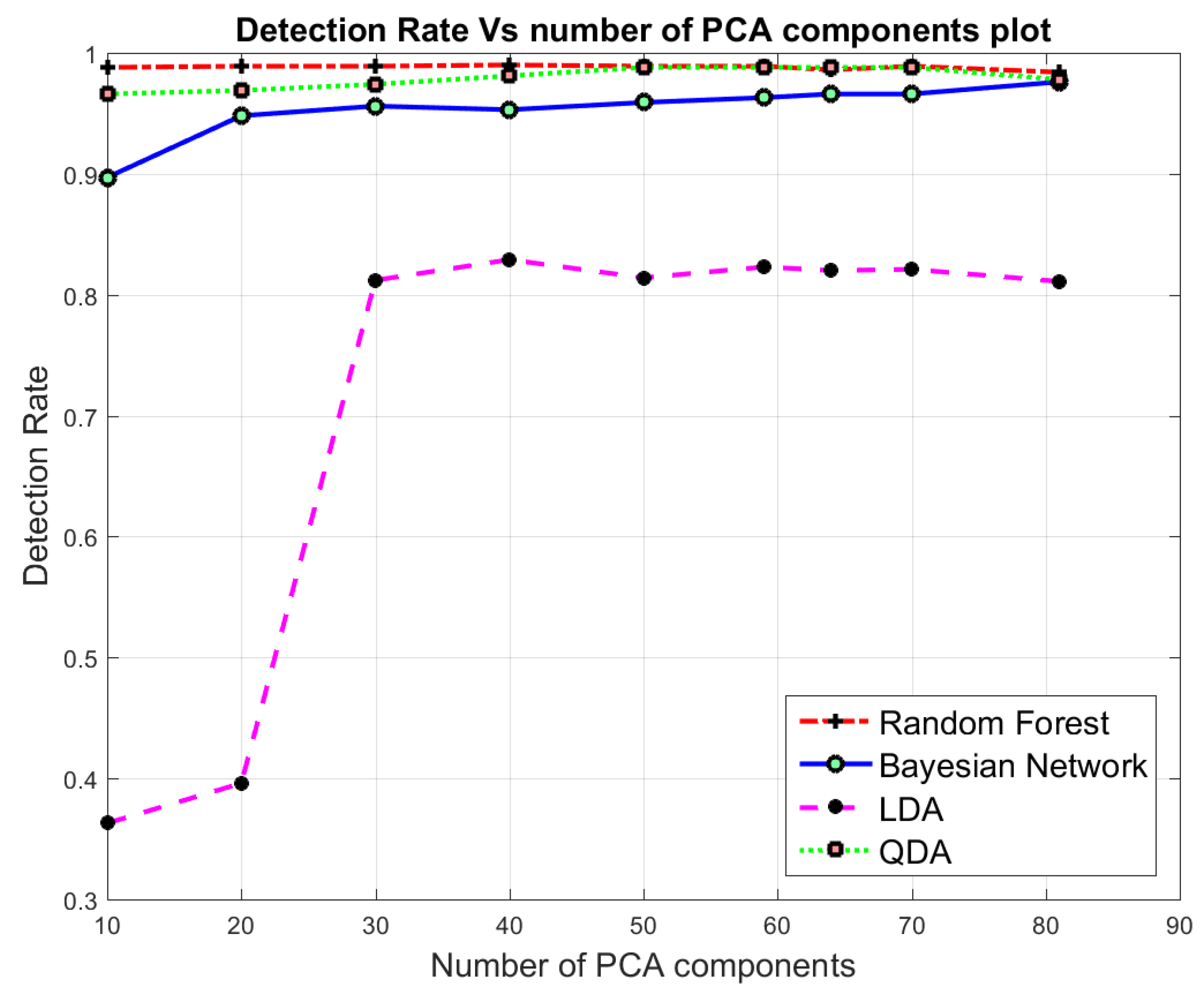
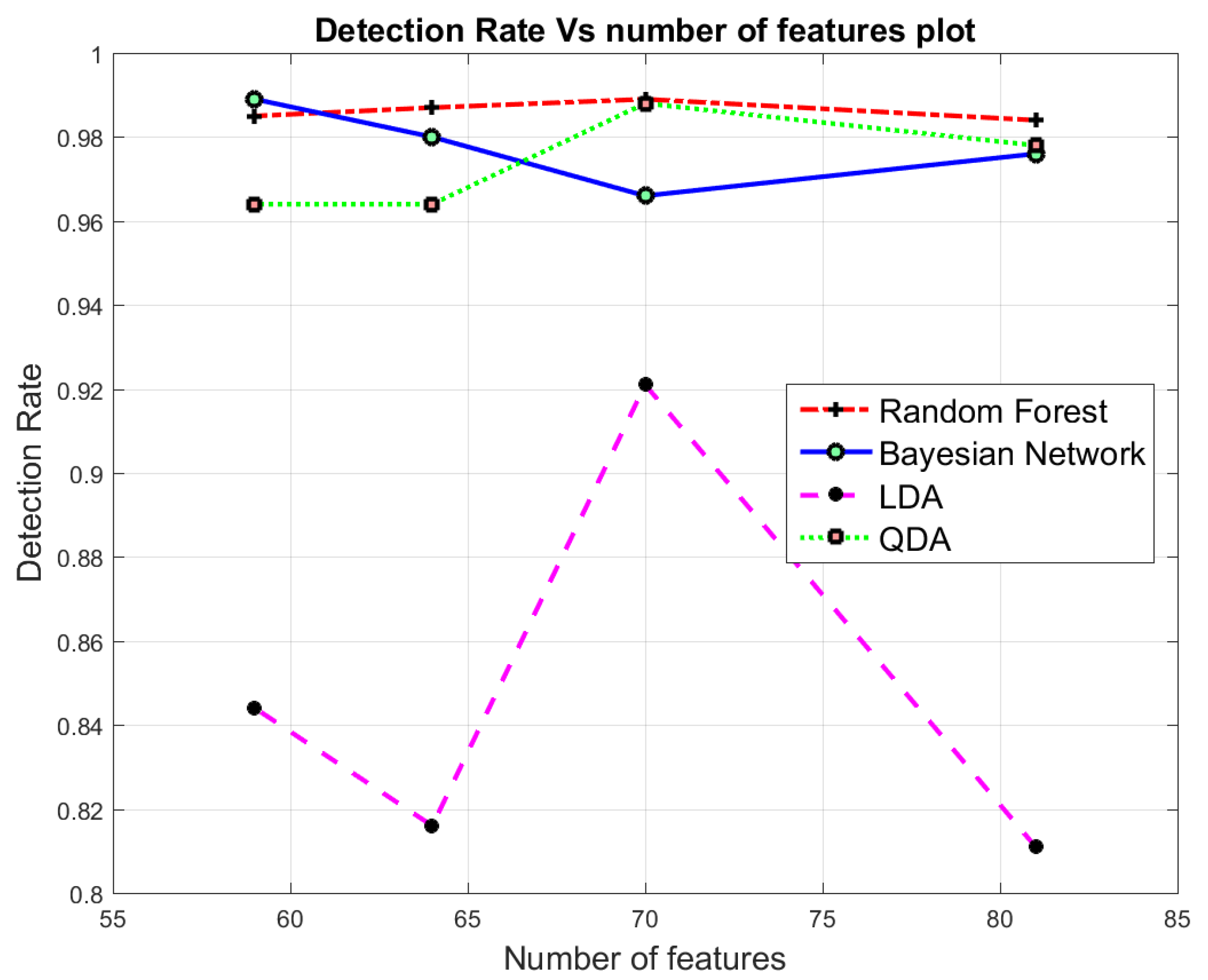
Figure 3 highlights the achieved detection rates resulted from the dimensionality reduction using PCA, whereas, Figure 4 shows the achieved detection rate using the reduced features set by AE. From Figure 3 and Figure 4, it is apparent that Random forest, QDA and Bayesian Network reported significantly higher detection rates than the LDA for the reduced feature dimensionality of CICIDS2017 using the PCA approach. The results from the classification using different classifiers assures that our reconstructing of new feature representation was good enough to achieve an overall accuracy of 98.5% with 59 features in binary classification using Random Forest from AE.

7.3. Multi-Class Classification

The study used the Acc, F-M, FPR, TPR, Precision, Recall, and the Combined multi-class metrics to evaluate the performance of multi-class classification.

Table 10. Performance evaluation of the proposed framework in multi-class classification using PCA.

	${(\mathit{PCA}-\mathit{RF})}_{\mathit{Mc}-\mathit{X}}$			${(\mathit{PCA}-\mathit{BN})}_{\mathit{Mc}-\mathit{X}}$			${(\mathit{PCA}-\mathit{LDA})}_{\mathit{Mc}-\mathit{X}}$			${(\mathit{PCA}-\mathit{QDA})}_{\mathit{Mc}-\mathit{X}}$
	Acc	F-M	${\mathit{CM}}_{\mathit{Mc}}$	Acc	F-M	${\mathit{CM}}_{\mathit{Mc}}$	Acc	F-M	${\mathit{CM}}_{\mathit{Mc}}$	Acc	F-M	${\mathit{CM}}_{\mathit{Mc}}$
81	0.985	0.995	0.986	0.930	0.953	0.925	0.901	0.914	0.801	0.972	0.974	0.961
70	0.996	0.988	0.988	0.948	0.964	0.942	0.894	0.906	0.735	0.967	0.975	0.967
64	0.996	0.997	0.986	0.949	0.966	0.955	0.893	0.906	0.745	0.967	0.975	0.985
59	0.996	0.995	0.987	0.952	0.967	0.917	0.893	0.906	0.677	0.967	0.975	0.880
50	0.996	0.996	0.987	0.924	0.941	0.916	0.859	0.880	0.679	0.927	0.946	0.885
40	0.996	0.997	0.9884	0.964	0.974	0.954	0.890	0.546	0.727	0.966	0.974	0.967
30	0.996	0.997	0.988	0.960	0.971	0.897	0.643	0.643	0.720	0.964	0.972	0.965
20	0.996	NAN	0.987	0.987	0.952	0.855	0.859	NAN	0.4805	0.892	0.886	0.886
10	0.996	NAN	0.986	0.953	0.964	0.946	0.850	NAN	0.363	0.856	0.886	0.886

and

Table 11. Performance evaluation of the proposed framework in multi-class classification using AE.

	${(\mathit{AE}-\mathit{RF})}_{\mathit{Mc}-\mathit{X}}$			${(\mathit{AE}-\mathit{BN})}_{\mathit{Mc}-\mathit{X}}$			${(\mathit{AE}-\mathit{LDA})}_{\mathit{Mc}-\mathit{X}}$			${(\mathit{AE}-\mathit{QDA})}_{\mathit{Mc}-\mathit{X}}$
	Acc	F-M	${\mathit{CM}}_{\mathit{Mc}}$	Acc	F-M	${\mathit{CM}}_{\mathit{Mc}}$	Acc	F-M	${\mathit{CM}}_{\mathit{Mc}}$	Acc	F-M	${\mathit{CM}}_{\mathit{Mc}}$
81	0.985	0.995	0.983	0.930	0.953	0.895	0.912	0.922	0.908	0.968	0.969	0.920
70	0.996	0.996	0.959	0.953	0.996	0.913	0.894	0.906	0.875	0.960	0.970	0.931
64	0.996	0.996	0.985	0.955	0.968	0.954	0.900	0.908	0.743	0.960	0.969	0.963
59	0.995	0.995	0.983	0.956	0.969	0.958	0.849	0.906	0.737	0.961	0.969	0.963

display the summary of the results obtained for the dimensionality reduction of the features for CICIDS2017 from 81 to 10 using PCA, and from 81 to 59 using AE, respectively.

Figure 5 presents the resulting accuracies in terms of the number of principle components. What is striking about the resulting accuracies in Figure 5 is that the Random Forest classifier shows a constantly high accuracy for reduced features from 81 through 10. In contrast, the resulting accuracies of LDA and QDA cases were oscillatory. For QDA, the accuracy is wobbling between 66% with 10 features and 96.7% with 60 features. For LDA with 10 and 40 features, the accuracy is fluctuating between 85% and 96.6%, respectively.

The results of the AE dimensionalty reduction approach are displayed in Figure 6. The observed accuracy for Random Forest is significant compared to LDA, QDA and the Bayesian Network classifiers. Furthermore, what stands out in this Figure 6, is the increase of the resulting accuracy for LDA for the reduced dimensionality from 81 through 59 features. Here, the AE reconstructed a new and reduced feature representation pattern that reflects the original data with minimum error. Unlike features selection techniques where the set of features made by feature selection is a subset of the original set of features that can be identified precisely, AE generated new features pattern with reduced dimensions.

A detailed analysis summary of the proposed framework in terms of False Positive Rate (FPR), True Positive Rate (TPR), Precision and Recall are tabulated in

Table 12. Performance evaluation before applying UDBB.

	(${\mathit{PCA}-\mathit{RF})}_{\mathit{Mc}-10}$ Original Distribution
	Recall	Precision	FP Rate	TP Rate
Benign	0.998	0.998	0.012	0.998
FTP-Patator	1.000	1.000	0.000	1.000
SSH-Patator	0.996	0.996	0.000	0.996
DDoS	0.877	0.900	0.001	0.877
HeartBleed	NAN	NAN	0.000	0.000
PortScan	1.000	0.998	0.000	1.000
DoSHulk	1.000	1.000	0.000	1.000
DoSGoldenEye	0.979	0.995	0.000	0.979
WebAttack: Brute Force	0.813	0.878	0.000	0.814
WebAttack:XSS	0.750	0.665	0.000	0.750
Infiltration	0.250	1.000	0.000	0.250
WebAttack:SQL	0.000	0.000	0.000	0.000
Botnet	0.960	0.991	0.000	0.960
Dos Slow HTTP Test	0.993	0.996	0.000	0.993
DoS Slow Loris	0.991	0.999	0.000	0.991
Weighted Average	0.996	0.965	0.010	0.996

and

Table 13. Performance evaluation after applying UDBB.

	(${\mathit{PCA}-\mathit{RF})}_{\mathit{Mc}-10}$ UDBB
	Recall	Precision	FP Rate	TP Rate
Benign	1.000	1.000	0.000	1.000
FTP-Patator	1.000	1.000	0.000	1.000
SSH-Patator	1.000	1.000	0.000	1.000
DDoS	1.000	1.000	0.000	1.000
HeartBleed	1.000	1.000	0.000	1.000
PortScan	1.000	0.999	0.000	1.000
DoSHulk	0.999	1.000	0.000	0.999
DoSGoldenEye	1.000	1.000	0.000	1.000
WebAttack: Brute Force	0.945	0.891	0.008	0.945
WebAttack:XSS	0.884	0.943	0.004	0.884
Infiltration	1.000	1.000	0.000	1.000
WebAttack:SQL	1.000	0.998	0.000	1.000
Botnet	1.000	1.000	0.000	1.000
Dos Slow HTTP Test	0.999	0.999	0.000	0.999
DoS Slow Loris	0.999	0.999	0.000	0.999
Weighted Average	0.988	0.989	0.001	0.988

. Table 12 depicts the results with 10 features (before applying UDBB), while Table 13 shows the results using 10 features (after applying UDBB). The weighted average result for all the attacks are presented in bold.

The results confirmed that the proposed framework with the reduced feature dimensionality achieved a maximum precision value of 0.996 and an FPR of 0.010, confirming the efficiency and effectiveness of the intrusion detection process. However, (${PCA-RF)}_{Mc-10}$ is unable to detect the HeartBleed attacks (noted as NAN in Table 12). In this Table, the Recall and Precision values for HeartBleed and WebAttack:SQL are 0.00, 0.000 and 0.000, 0.000, respectively. A justification of such outcome could be due to the fact that the number of instances of HeartBleed and WebAttack:SQL originally embedded in CICIDS2017 is equal to 11 and 21, respectively. This is expected, since the total number of HeartBleed instances in the original dataset is 11 instances. Thus, these instances were miss-classified by the classifier. To resolve this issue and to assure that the achieved accuracy is reflected due to the effective reduction approach, this paper applies the uniform distribution-based balancing technique to overcome the imbalanced class distributions of certain attacks in CICIDS2017.

Table 14. Performance evaluation of ${(PCA-X)}_{Mc-10}$.

Classifier	Acc	F-M	${\mathit{CM}}_{(\mathit{Mc})}$
Before applying UDBB
PCA-Random Forest (${PCA-RF)}_{Mc-10}$	0.996	NAN	0.9866
PCA-Bayesian Network (${PCA-BN)}_{Mc-10}$	0.953	0.964	0.9464
PCA-LDA (${PCA-LDA)}_{Mc-10}$	0.850	NAN	0.3626
PCA-QDA (${PCA-QDA)}_{Mc-10}$	0.856	0.886	0.8862
After applying UDBB
PCA-Random Forest (${PCA-RF)}_{Mc-10}$	0.988	0.988	0.9882
PCA-Bayesian Network (${PCA-BN)}_{Mc-10}$	0.976	0.977	0.9839
PCA-LDA (${PCA-LDA)}_{Mc-10}$	0.957	0.957	0.6791
PCA-QDA (${PCA-QDA)}_{Mc-10}$	0.989	0.990	0.8851

shows the performance before and after applying the UDBB approach. As observed, (${PCA-RF)}_{Mc-10}$ achieved 99.6% and 98.8% before and after applying UDBB, respectively. In the same manner, (${PCA-QDA)}_{Mc-10}$ achieved 85.6% and 98.9% before and after applying UDBB, respectively. The highest achieved F-M was obtained by (${PCA-QDA)}_{Mc-10}$. However, the highest $C{M}_{(Mc)}$ achieved was 98.6% by (${PCA-RF)}_{Mc-10}$.

The performance evaluation of (${PCA-X)}_{Bc-10}$ and (${PCA-X)}_{Mc-10}$ in terms of the time to build and test the model is presented in

Table 15. Time to build and test the models.

Classifier	Time to Build the Model (Sec.)	Time to Test the Model (Sec.)
Binary-class Classification
LDA	12.16	5.56
QDA	12.84	6.57
RF	752.67	21.52
BN	199.17	11.07
Multi-class Classification
LDA	17.5	2.96
QDA	15.35	3.16
RF	502.81	41.66
BN	175.17	10.07

(X represents the classifier). The lowest times to test the model were achieved by LDA with 2.96 s for multi-class and 5.56 s for binary class classification.

Here, the Random Forest classifier that has the best detection performance, comes with the highest overhead in terms of the time to build and test the model. The fundamental notion behind Random Forest is that it combines many decision trees into a single model and specifically in this work, the dataset has over 2.5 million instances in total. This is expected since the worst case time complexity of Random Forest is estimated using Equation (22) [48].

$$O(MK{N}^{2}logN)$$

(22)

where K is the number of trees, M is the number of variables used in each split, and N is the number of training samples.

Moreover, a visualization of the dataset with two PCA components before and after applying the distribution-based balancing approach is displayed in Figure 7 and Figure 8.

This observation of the CICIDS2017 dataset visually represents how the instances are set apart. As displayed in Figure 8, the same type of instances were positioned (clustered) together in groups. This shows a significant improvement over the PCA visualization before applying UDBB. Here, the normal instances are very clearly clustered in their own group. This is applied for other types of instances as well.

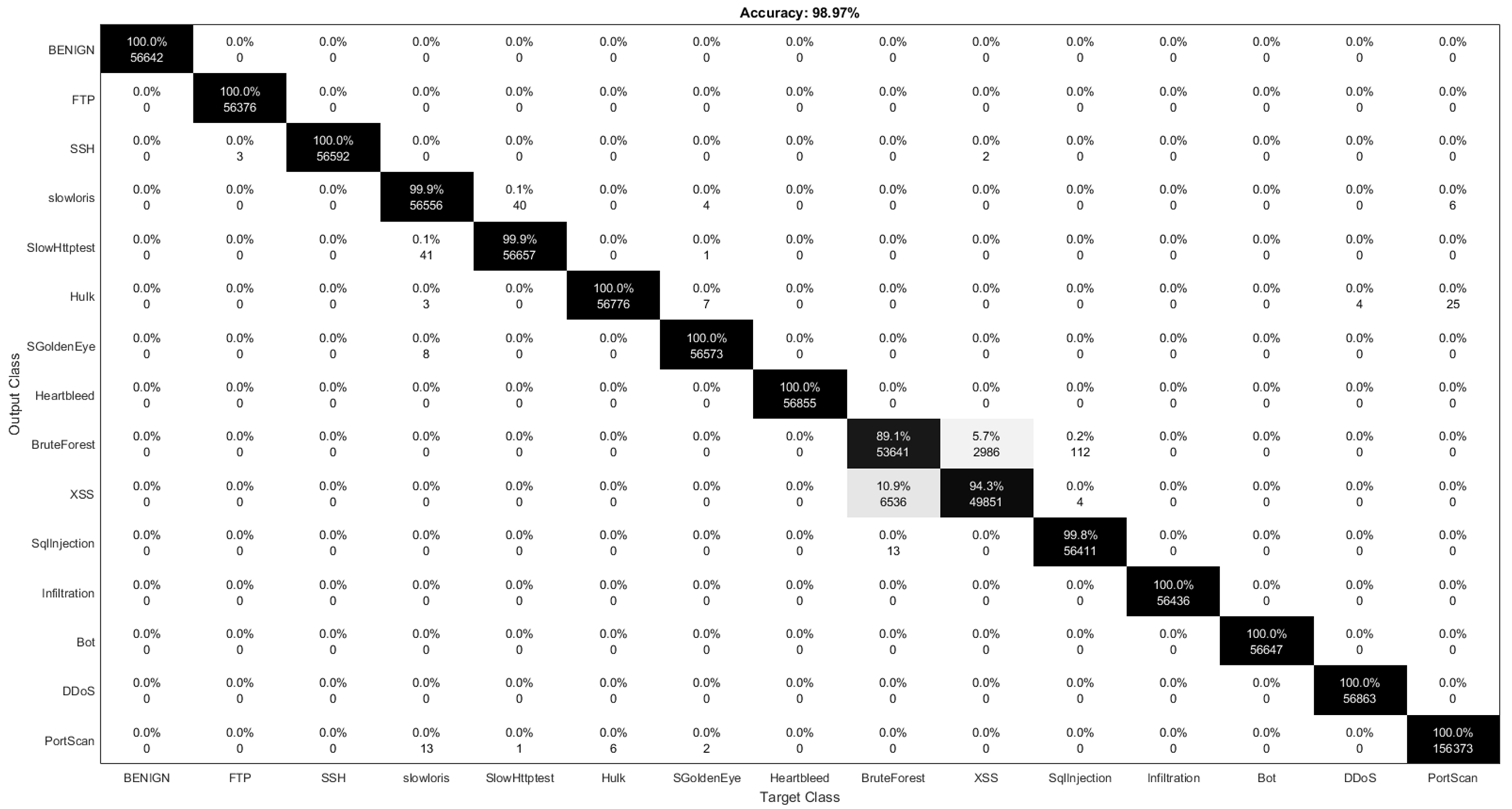
The confusion matrix for the $PCA-R{F}_{Mc-10}$ is shown in Figure 9. The value for HeartBleed is reported as NAN (Not A Number). These values result from operations which have undefined numerical values. The classifier $PCA-R{F}_{Mc-10}$ fails to classify HeartBleed attacks. In contrast, as a result of applying the UDBB technique, the $PCA-R{F}_{Mc-10}$ is able to detect 100% of HeartBleed attacks, as indicated from the confusion matrix in Figure 10.

A comparison between the proposed framework and related work is highlighted in

Table 16. A comparison of the proposed framework and previous studies.

Reference	Classifier Name	F-Measure	Feature
			Selection/Extraction
			(Features Count)
[4]	KNN	0.96	Random Forest
	RF	0.97	Regressor (54)
	ID3	0.98
	Adaboost	0.77
	MLP	0.76
	Naïve Bayes	0.04
	QDA	0.92
[13]	MLP	0.948	Payload related
			features
[15]	SVM	0.921	DBN
[14]	KNN	0.997	Fisher Scoring (30)
[51]	XGBoost	0.995	(80)
	for DoS Attacks
[49]	Deep Learning	Accuracy	(80)
	for Port Scan Attacks	97.80
[49]	SVM	Accuracy	(80)
	for Port Scan Attacks	69.79
[17]	XGBoost	Accuracy	DDR Features
		98.93	Selections (36)
[50]	Deep Multi Layer	Accuracy	Recursive feature
	Perceptron (DMLP)	91.00	elimination
	for DDoS Attacks		with Random Forest
Proposed
Framework	Random Forest	0.995	Auto-encoder (59)
Proposed		PCA with Original
Framework	Random Forest	0.996	Distribution (10)
Proposed		PCA With
Framework	Random Forest	0.988	UDBB(10)

. The authors in [17,49,50] reported the accuracy. Our proposed framework outperforms previous studies in terms of F-Measure and accuracy.

8. Challenges and Limitations

Although this study has successfully demonstrated the significance of the feature dimensionality reduction techniques which led to better results in terms of several performance metrics as well classification speeds for an IDS, it has certain limitations and challenges which are summarized as follows.

8.1. Fault Tolerance

Fault tolerance enables a system to continue operating properly in the event of failure or faults within any of its components. Fault tolerance can be achieved through several techniques. One aspect of fault tolerance in our system is the ability of the designed approach to detect a large set of well-known attacks. Our models have been trained to detect the 14 up-to-date and well-known type of attacks. Furthermore, fault tolerance can be achieved by adopting the majority voting technique [52]. The trained models of Random Forest, Bayesian Network, and LDA can be used in a majority voting-based intrusion detection system that can adapt fault tolerance. Moreover, the deployment of distributed intrusion detection systems in the network can enable fault tolerance.

8.2. Adaption to Non-Stationary Traffic/Nonlinear Models

The AE has the ability to represent models that are linear and nonlinear. Moreover, once the model is trained, it can be used for non-stationary traffic. We intend to further extend our work in the future with an online anomaly-based intrusion detection system.

8.3. Model Resilience

As presented in Table 12 and Table 13, the achieved FP rate is 0.010 and 0.001 respectively, which may reflect a built-in attack resiliency. Moreover, our models were trained in an offline manner. This ensures that an adversary cannot inject misclassified instances during the training phase. On the contrary, such case could occur with online-trained models. Therefore, it is essential for the machine learning system employed in intrusion detection to be resilient to adversarial attacks [53]. An approach to quantify the resilience of machine learning classifiers was introduced in [53]. The association of these factors will be investigated in future studies.

8.4. Ease of Dataset Acquisition/Model Building

The data used for our IDS model was acquired from the CICIDS2017 dataset which is a publicly available dataset provided by the Canadian Institute for Cybersecurity [35,36]. The dataset is open source and available for download and sharing.

8.5. Quality of Experience

According to [54], the Quality of Experience is used to measure and express, preferably as numerical values, the experience and perception of the users with a service or application software. The current research was not specifically designed to evaluate factors related to Quality of Experience. Future directions of this research may include such investigations.

9. Conclusion and Future Work

The aim of this research was to examine incorporating auto-encoder and PCA for dimensionality reduction and the use of classifiers towards designing an efficient network intrusion detection system on the CICIDS2017 dataset. The experimental analysis confirmed the significance of the feature dimensionality reduction techniques which led to better results in terms of several performance metrics as well as classification speeds. These findings highlight the potential usefulness of auto-encoder and PCA in dimensionality reduction for IDS. From our experiments, we found that PCA is superior, faster, more interpretable and can reduce the dimensionality of the data to as few as two components. The long training time and limited computational resources formed a barrier towards reducing the dimensionality beyond 59 features representation for the AE approach. This study suggests that AE can be used when the data necessitates a highly non-linear feature representation.

The large number of decision trees that the Random Forest classifier produced by randomly selecting a subset of training samples and a subset of variables for splitting at each tree node, makes the Random Forest classifier less sensitive to both the quality of training instances as well as the overfitting issue. Moreover, Random Forest is suitable, robust, and stable to classify high dimensional and correlated data. These explanations provide a justification as to why Random Forest yielded better results in comparison with other classifiers [55].

As exemplified by the obtained results, the PCA approach is able to preserve important information in CICIDS2017, while efficiently reducing the features dimensions in the used dataset, as well as presenting a reasonable visualization model of the data. Features such as Subflow Fwd Bytes, Flow Duration, Flow Inter arrival time (IAT), PSH Flag Count, SYN Flag Count, Average Packet Size, Total Len Fwd Pck, Active Mean and Min, ACK Flag Count, and Init_Win_bytes_fwd are observed to be the discriminating features embedded in CICIDS2017 [4]. Regarding this study, PCA was very efficient and produced better results than AE. In comparison with AE, the PCA approach is restricted to a linear mapping, whereas the AE can have a nonlinear encoder/decoder architecture.

As a future direction, this research will also serve as a base for further studies and investigations towards developing efficient IDS’s from various intrusion detection datasets. Furthermore, the trained models could be extended to implement an IDS for online anomaly-based detection.

References

- Albanese, M.; Erbacher, R.F.; Jajodia, S.; Molinaro, C.; Persia, F.; Picariello, A.; Sperlì, G.; Subrahmanian, V. Recognizing unexplained behavior in network traffic. In Network Science and Cybersecurity; Springer: Berlin, Germany, 2014; pp. 39–62. [Google Scholar]
- Abdulhammed, R.; Faezipour, M.; Elleithy, K. Intrusion Detection in Self organizing Network: A Survey. In Intrusion Detection and Prevention for Mobile Ecosystems; Kambourakis, G., Shabtai, A., Kolias, C., Damopoulos, D., Eds.; CRC Press Taylor & Francis Group: New York, NY, USA, 2017; Chapter 13; pp. 393–449. [Google Scholar]
- Lee, C.H.; Su, Y.Y.; Lin, Y.C.; Lee, S.J. Machine learning based network intrusion detection. In Proceedings of the 2017 2nd IEEE International Conference on Computational Intelligence and Applications (ICCIA), Beijing, China, 8–11 September 2017; pp. 79–83. [Google Scholar]
- Sharafaldin, I.; Lashkari, A.H.; Ghorbani, A.A. Toward generating a new intrusion detection dataset and intrusion traffic characterization. In Proceedings of the Fourth International Conference on Information Systems Security and Privacy, ICISSP, Funchal, Madeira, Portugal, 22–24 January 2018. [Google Scholar]
- Sorzano, C.O.S.; Vargas, J.; Montano, A.P. A survey of dimensionality reduction techniques. arXiv, 2014; arXiv:1403.2877. [Google Scholar]
- Fodor, I.K. A Survey of Dimension Reduction Techniques; Center for Applied Scientific Computing, Lawrence Livermore National Laboratory: Livermore, CA, USA, 2002; Volume 9, pp. 1–18. [Google Scholar]
- Rosaria, S.; Adae, I.; Aaron, H.; Michael, B. Seven Techniques for Dimensionality Reduction; KNIME: Zurich Switzerland, 2014. [Google Scholar]
- Van Der Maaten, L.; Postma, E.; Van den Herik, J. Dimensionality reduction: A comparative review. J. Mach. Learn. Res. 2009, 10, 66–71. [Google Scholar]
- Bertens, P. Rank Ordered Autoencoders. arXiv, 2016; arXiv:1605.01749. [Google Scholar]
- Vijayan, R.; Devaraj, D.; Kannapiran, B. Intrusion detection system for wireless mesh network using multiple support vector machine classifiers with genetic-algorithm-based feature selection. Comput. Secur. 2018, 77, 304–314. [Google Scholar] [CrossRef]
- Radford, B.J.; Richardson, B.D. Sequence Aggregation Rules for Anomaly Detection in Computer Network Traffic. arXiv, 2018; arXiv:1805.03735. [Google Scholar]
- Lavrova, D.; Semyanov, P.; Shtyrkina, A.; Zegzhda, P. Wavelet-analysis of network traffic time-series for detection of attacks on digital production infrastructure. SHS Web Conf. EDP Sci. 2018, 44, 00052. [Google Scholar] [CrossRef]
- Watson, G. A Comparison of Header and Deep Packet Features When Detecting Network Intrusions; Technical Report; University of Maryland: College Park, MD, USA, 2018. [Google Scholar]
- Aksu, D.; Üstebay, S.; Aydin, M.A.; Atmaca, T. Intrusion Detection with Comparative Analysis of Supervised Learning Techniques and Fisher Score Feature Selection Algorithm. In International Symposium on Computer and Information Sciences; Springer: Berlin, Germany, 2018; pp. 141–149. [Google Scholar]
- Marir, N.; Wang, H.; Feng, G.; Li, B.; Jia, M. Distributed Abnormal Behavior Detection Approach based on Deep Belief Network and Ensemble SVM using Spark. IEEE Access 2018. [Google Scholar] [CrossRef]
- Spark, A. PySpark 2.4.0 Documentation. 2018. Available online: https://spark.apache.org/docs/latest/api/python/index.html (accessed on 10 November 2018).
- Bansal, A. DDR Scheme and LSTM RNN Algorithm for Building an Efficient IDS. Master’s Thesis, Thapar Institute of Engineering and Technology, Punjab, India, 2018. [Google Scholar]
- Chen, T.; He, T.; Benesty, M. Xgboost: Extreme Gradient Boosting. R Package Version 0.4-2. 2015, pp. 1–4. Available online: http://cran.fhcrc.org/web/packages/xgboost/vignettes/xgboost.pdf (accessed on 11 March 2019).
- Hothorn, T.; Hornik, K.; Zeileis, A. Ctree: Conditional Inference Trees. The Comprehensive R Archive Network. 2015. Available online: https://cran.r-project.org/web/packages/partykit/vignettes/ctree.pdf (accessed on 23 January 2019).
- Aminanto, M.E.; Choi, R.; Tanuwidjaja, H.C.; Yoo, P.D.; Kim, K. Deep abstraction and weighted feature selection for Wi-Fi impersonation detection. IEEE Trans. Inf. Forensics Secur. 2018, 13, 621–636. [Google Scholar] [CrossRef]
- Zhu, J.; Ming, Y.; Song, Y.; Wang, S. Mechanism of situation element acquisition based on deep auto-encoder network in wireless sensor networks. Int. J. Distrib. Sens. Netw. 2017, 13. [Google Scholar] [CrossRef] [Green Version]
- Al-Qatf, M.; Lasheng, Y.; Alhabib, M.; Al-Sabahi, K. Deep Learning Approach Combining Sparse Autoen-coder with SVM for Network Intrusion Detection. IEEE Access 2018, 6, 52843–52856. [Google Scholar] [CrossRef]
- Tavallaee, M.; Bagheri, E.; Lu, W.; Ghorbani, A.A. Nsl-Kdd Dataset. 2012. Available online: http://www.unb.ca/research/iscx/dataset/iscx-NSL-KDD-dataset.html (accessed on 28 February 2016).
- Bay, S.D.; Kibler, D.; Pazzani, M.J.; Smyth, P. The UCI KDD archive of large data sets for data mining research and experimentation. ACM SIGKDD Explor. Newsl. 2000, 2, 81–85. [Google Scholar] [CrossRef] [Green Version]
- Javaid, A.; Niyaz, Q.; Sun, W.; Alam, M. A deep learning approach for network intrusion detection system. In Proceedings of the 9th EAI International Conference on Bio-inspired Information and Communications Technologies (formerly BIONETICS), ICST (Institute for Computer Sciences, Social-Informatics and Telecommunications Engineering), Cotonou, Benin, 24 May 2016; pp. 21–26. [Google Scholar]
- Min, E.; Long, J.; Liu, Q.; Cui, J.; Cai, Z.; Ma, J. SU-IDS: A Semi-supervised and Unsupervised Framework for Network Intrusion Detection. In International Conference on Cloud Computing and Security; Springer: Cham, Switzerland, 2018; pp. 322–334. [Google Scholar]
- Xia, D.; Yang, S.; Li, C. Intrusion Detection System Based on Principal Component Analysis and Grey Neural Networks. In Proceedings of the 2010 Second International Conference on Networks Security, Wireless Communications and Trusted Computing, Wuhan, Hubei, China, 24–25 April 2010; Volume 2, pp. 142–145. [Google Scholar] [CrossRef]
- Vasan, K.K.; Surendiran, B. Dimensionality reduction using Principal Component Analysis for network intrusion detection. Perspect. Sci. 2016, 8, 510–512. [Google Scholar] [CrossRef] [Green Version]
- Shiravi, A.; Shiravi, H.; Tavallaee, M.; Ghorbani, A.A. Toward developing a systematic approach to generate benchmark datasets for intrusion detection. Comput. Secur. 2012, 31, 357–374. [Google Scholar] [CrossRef]
- Aminanto, M.E.; Kim, K. Improving Detection of Wi-Fi Impersonation by Fully Unsupervised Deep Learning. In Proceedings of the Information Security Applications: 18th International Workshop (WISA 2017), Jeju Island, Korea, 24–26 August 2017. [Google Scholar]
- Aminanto, M.E.; Kim, K. Detecting Active Attacks in WiFi Network by Semi-supervised Deep Learning. In Proceedings of the Conference on Information Security and Cryptography 2017 Winter, Sochi, Russian Federation, 8–10 September 2017. [Google Scholar]
- Kolias, C.; Kambourakis, G.; Stavrou, A.; Gritzalis, S. Intrusion detection in 802.11 networks: Empirical evaluation of threats and a public dataset. IEEE Commun. Surv. Tutor. 2016, 18, 184–208. [Google Scholar] [CrossRef]
- Vilela, D.W.; Ed’Wilson, T.F.; Shinoda, A.A.; de Souza Araujo, N.V.; de Oliveira, R.; Nascimento, V.E. A dataset for evaluating intrusion detection systems in IEEE 802.11 wireless networks. In Proceedings of the 2014 IEEE Colombian Conference on Communications and Computing (COLCOM), Bogota, Colombia, 4–6 June 2014; pp. 1–5. [Google Scholar]
- Ring, M.; Wunderlich, S.; Grüdl, D.; Landes, D.; Hotho, A. Flow-based benchmark data sets for intrusion detection. In Proceedings of the 16th European Conference on Cyber Warfare and Security, Dublin, Ireland, 29–30 June 2017; pp. 361–369. [Google Scholar]
- Canadian Institute of Cybersecurity, University of New Brunswick. CICFlowMeter. 2017. Available online: https://www.unb.ca/cic/research/applications.html#CICFlowMeter (accessed on 23 January 2019).
- CIC. Canadian Institute of Cybersecurity. List of Extracted Traffic Features by CICFlowMeter-V3. 2017. Available online: https://www.unb.ca/cic/datasets/ids-2017.html (accessed on 23 January 2019).
- Kingma, D.P.; Welling, M. Auto-encoding variational bayes. arXiv, 2013; arXiv:1312.6114. [Google Scholar]
- Rezende, D.J.; Mohamed, S.; Wierstra, D. Stochastic backpropagation and approximate inference in deep generative models. arXiv, 2014; arXiv:1401.4082. [Google Scholar]
- Sakurada, M.; Yairi, T. Anomaly detection using autoencoders with nonlinear dimensionality reduction. In Proceedings of the MLSDA 2014 2nd Workshop on Machine Learning for Sensory Data Analysis, Gold Coast, QLD, Australia, 2 December 2014; p. 4. [Google Scholar]
- Makhzani, A. Unsupervised Representation Learning with Autoencoders. Ph.D. Thesis, University of Toronto, Toronto, ON, Canada, 2018. [Google Scholar]
- Mirsky, Y.; Doitshman, T.; Elovici, Y.; Shabtai, A. Kitsune: An ensemble of autoencoders for online network intrusion detection. arXiv, 2018; arXiv:1802.09089. [Google Scholar]
- Johnstone, I.M.; Lu, A.Y. Sparse principal components analysis. arXiv, 2009; arXiv:0901.4392. [Google Scholar]
- Espíndola, R.; Ebecken, N. On extending f-measure and g-mean metrics to multi-class problems. WIT Trans. Inf. Commun. Technol. 2005, 35. [Google Scholar] [CrossRef]
- García, V.; Sánchez, J.S.; Mollineda, R.A. On the effectiveness of preprocessing methods when dealing with different levels of class imbalance. Knowl.-Based Syst. 2012, 25, 13–21. [Google Scholar] [CrossRef] [Green Version]
- Hamed, T.; Dara, R.; Kremer, S.C. Network intrusion detection system based on recursive feature addition and bigram technique. Comput. Secur. 2018, 73, 137–155. [Google Scholar] [CrossRef]
- Bermejo, P.; Gámez, J.A.; Puerta, J.M. Improving the performance of Naive Bayes multinomial in e-mail foldering by introducing distribution-based balance of datasets. Expert Syst. Appl. 2011, 38, 2072–2080. [Google Scholar] [CrossRef]
- Abdulhammed, R.; Faezipour, M.; Abuzneid, A.; AbuMallouh, A. Deep and Machine Learning Approaches for Anomaly-Based Intrusion Detection of Imbalanced Network Traffic. IEEE Sens. Lett. 2019, 3, 7101404. [Google Scholar] [CrossRef]
- Louppe, G. Understanding Random Forests: From Theory to Practice. Ph.D. Thesis, University of Liège, Belgium, 2014. [Google Scholar]
- Aksu, D.; Aydin, M.A. Detecting Port Scan Attempts with Comparative Analysis of Deep Learning and Support Vector Machine Algorithms. In Proceedings of the 2018 International Congress on Big Data, Deep Learning and Fighting Cyber Terrorism (IBIGDELFT), Ankara, Turkey, 3–4 December 2018; pp. 77–80. [Google Scholar]
- Ustebay, S.; Turgut, Z.; Aydin, M.A. Intrusion Detection System with Recursive Feature Elimination by Using Random Forest and Deep Learning Classifier. In Proceedings of the 2018 International Congress on Big Data, Deep Learning and Fighting Cyber Terrorism (IBIGDELFT), Ankara, Turkey, 3–4 December 2018; pp. 71–76. [Google Scholar]
- Bansal, A.; Kaur, S. Extreme Gradient Boosting Based Tuning for Classification in Intrusion Detection Systems. In International Conference on Advances in Computing and Data Sciences; Springer: Singapore, 2018; pp. 372–380. [Google Scholar]
- Kaur, P.; Rattan, D.; Bhardwaj, A.K. An analysis of mechanisms for making ids fault tolerant. Int. J. Comput. Appl. 2010, 1, 22–25. [Google Scholar] [CrossRef]
- Viegas, E.; Santin, A.; Neves, N.; Bessani, A.; Abreu, V. A Resilient Stream Learning Intrusion Detection Mechanism for Real-time Analysis of Network Traffic. In Proceedings of the GLOBECOM 2017—2017 IEEE Global Communications Conference, Singapore, 4–8 December 2017; pp. 1–6. [Google Scholar]
- Al-Shehri, S.M.; Loskot, P.; Numanoglu, T.; Mert, M. Common Metrics for Analyzing, Developing and Managing Telecommunication Networks. arXiv, 2017; arXiv:1707.03290. [Google Scholar]
- Belgiu, M.; Drăguţ, L. Random forest in remote sensing: A review of applications and future directions. ISPRS J. Photogramm. Remote Sens. 2016, 114, 24–31. [Google Scholar] [CrossRef]
Figure 1.
Proposed Framework.
Figure 2.
The structure of an AE.
Figure 3.
Binary Class Classification: Detection Rate in terms of number of components using PCA.
Figure 4.
Binary Class Classification: Detection Rate in terms of number of features using Auto-Encoder.
Figure 5.
Multi Class Classification: Accuracy in terms of number of components using PCA.
Figure 6.
Multi Class Classification: Accuracy in terms of number of features using AE.
Figure 7.
2D Visualization of PCA on CICIDS2017 with original distribution.
Figure 8.
2D Visualization of PCA on CICIDS2017 with UDBB.
Figure 9.
Confusion Matrix for ( with original class distribution.
Figure 10.
Confusion Matrix for ( with UDBB.