Position Estimation of Automatic-Guided Vehicle Based on MIMO Antenna Array

Abstract

The existing positioning methods for the automatic guided vehicle (AGV) in the port can not achieve high location precision, Therefore, a novel multiple input multiple output (MIMO) antenna radar positioning scheme is proposed in this paper. The positioning problem for AGV is considered, and the joint estimation problem for direction of departure (DoD) and direction of arrival (DoA) is addressed in the multiple-input multiple-output (MIMO) radar system. With the radar detect the transponder and estimate the DoA/DoD, the relative location between the transponder and the AGV can be obtained. The corresponding Cramér–Rao lower bounds (CRLBs) for the target parameters are also derived theoretically. Finally, we compare the positioning accuracy of the traditional global position system (GPS) with the proposed MIMO radar system. Simulation results show that the proposed method can achieve better performance than the traditional GPS.

1. Introduction

The automatic guided vehicle (AGV) is widely used in modern intelligent ports or other industrial applications, which can safely moving materials to the rightful destination under the control of local area network [1,2]. The navigation of AGV mainly using vision, magnets, or lasers. Before the early 1980s, the embedded electromagnetic induction method was always the main guiding technology of AGV. With the development of electronic technology, new guiding technologies are constantly being researched and promoted. At present, the navigation of AGV including two types, the fixed path method and the free path method. The fixed path method is represented by magnetic navigation technology. Since the route is fixed, the path change and expansion is inconvenient. The free path method mainly includes laser position, visual position, millimeter wave radar method, inertial navigation system and global position system (GPS).

The laser position is based on the triangle localization method. By using some reflection sign, the laser scan the surrounding area and obtain the location information of the sign. The laser position has high precision, but is susceptible to weather and needs to install a large number of reflective signs. The machine vision navigation provides guidance through visual image processing that suitable for various scenes with high positioning accuracy. However, the cost of the systems is too high and the performance is greatly affected by image sensors. The inertial navigation system (INS) is a relative positioning method. A gyroscope is installed on the vehicle to accurately obtain the direction and speed of the trolley. When the coordinates of the starting position is known, the data of the trolley can be calculated. The system is simple and flexible with low cost and good real-time performance. The disadvantage is that the error accumulates due to various reasons, and long-term operation can lead to loss of precision completely. The GPS is a wireless navigation system that is positioned by navigation satellites. It can provide global, All-weather, continuous and real-time navigation and positioning. However, ordinary users can only use the standard positioning service (SPS) provided by GPS. The SPS accuracy is $\pm 10$ m on the horizontal plane, and the accuracy of AGV positioning requirement is 0.03 m∼0.1 m. The millimeter wave radar (MMWR) is place a millimeter wave radar on an AGV, the radar rotates to find a beacon installed at a known position, then uses the relative position information of the beacon to determine and continuously update the position of the AGV. The navigation accuracy of the method can reach $\pm 0.1$ m.

In this paper, the position of the AGV is addressed. Different from the above methods, a novel positioning method based on multiple input multiple output (MIMO) antenna array is proposed, where the direction of arrival (DoA) and direction of departure (DoD) is estimated to determine the position of the AGV. Additionally, we theoretically derive the corresponding Cramér-Rao lower bounds (CRLBs) for the target parameters. Then we compare the estimation performance of the traditional global position system (GPS) with the proposed MIMO radar system.

The remainder of the manuscript is organized as follows. The description of the proposed system is given in Section 2, and the system model is given in Section 3, the compressed sensing-based DoD and DoA estimation method is proposed in Section 4, The CRLB is given in Section 5. The simulation results are given in Section 6. Section 7 concludes the paper.

Notations:$\mathcal{E}\left\{·\right\}$ denotes the expectation operation, ${\mathit{I}}_P$ denotes a $P\times P$ identity matrix, ${\left(·\right)}^{⊺}$ denotes the matrix transposeand, ${\left(·\right)}^{\mathrm{H}}$ denotes the Hermitian transpose, $\mathcal{CN}\left(\mathbf{\mu },\mathit{R}\right)$ denotes the complex Gaussian distribution with the mean being $\mathbf{\mu }$ and the variance matrix being $\mathit{R}$, ${\parallel ·\parallel }_2$, ${\parallel ·\parallel }_0$, $\parallel ·\parallel$, ⊗, $vec\left\{·\right\}$ denote the ${\ell }_2$ norm, the ${\ell }_0$ norm, Frobenius norms, the Kronecker product, the vectorization of a matrix, respectively.

2. System Description

Figure 1 shows the AGV with an antenna frame for track guidance. With the aid of the transponder (L1) the deviation from the predetermined track is determined. With this information, an external computer is able to determine the new direction required to return to the predetermined track as soon as possible (the external computer is not part of the system). Rotary encoders enable changing the direction of travel whenever necessary. Thus, it is possible to switch tracks at predetermined points. Again, the AGV corrects its position independently upon reaching the next transponder.

When the antenna crosses a transponder, the transponder is supplied by a 128 KHz energy field and transmits its code number back to the reading antenna at half frequency. The relative transponder position rectangular to the direction of travel is measured. From this relative position it is not possible to derive a world coordinate system without further effort due to the fact, that the transponder field is rotationally symmetrical to the longitudinal axis of the transponder. The internal interpreter decodes the transponder code. Each exceeding of the coordinate axes in direction of travel generates a positioning impulse with adjustable duration. Due to the measuring principle different signal strengths of transponders and altitude variations of the antenna have hardly any influence on the output signal.

In 3-dimensional (3-D) space, in order to obtain the position of the AGV, three parameters including the x coordinate, y coordinate and the z coordinate should be determined. Since the height h between AGV and floor is a constant, We only need to estimate the x coordinate and y coordinate. As the distance between the AGV and transponder is very close (about 30 cm), the positioning accuracy can not be assured by measuring the distance or angles in the polar coordinates. Therefore, in this paper, multi-antenna array is adopted to estimate the DoD/DoA for precise positioning.

3. System Model

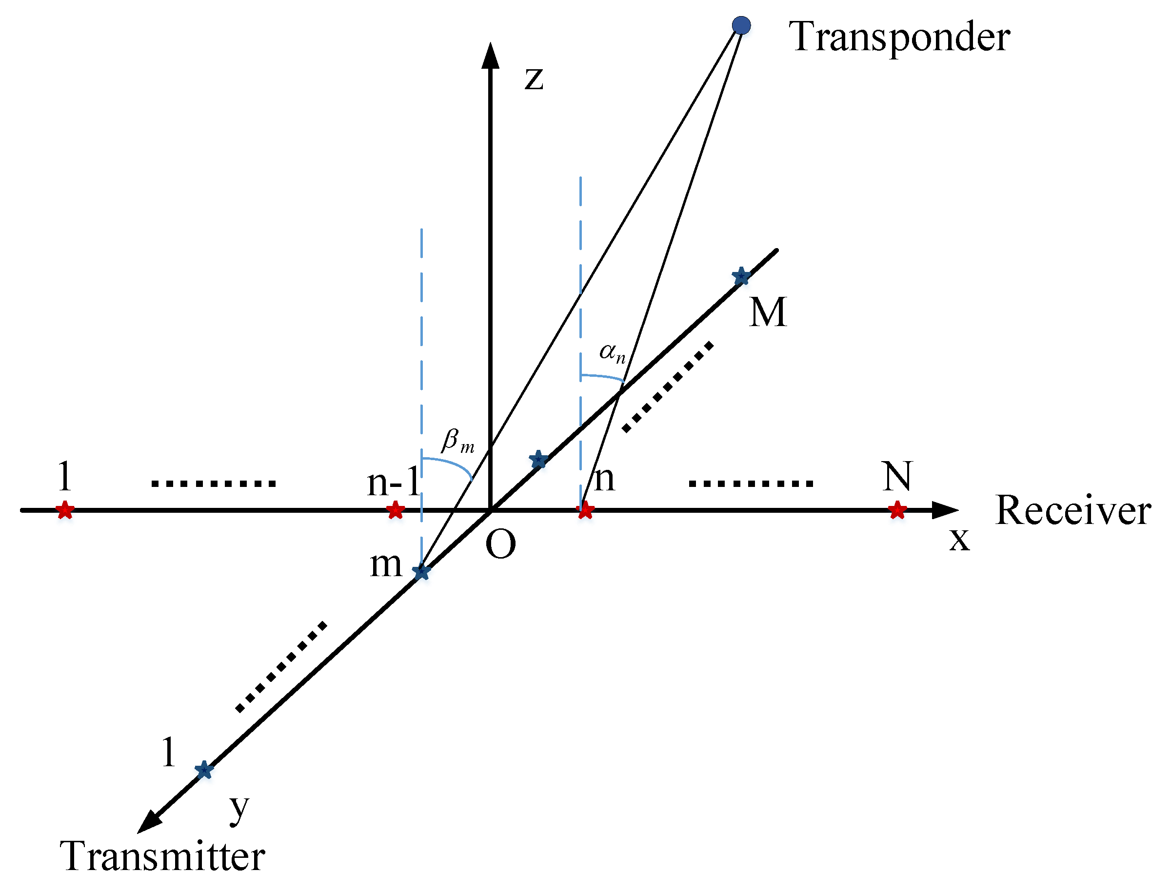
Consider a collocated MIMO radar with M element ULA as the transmitter and N element ULA as the receiver [3,4,5,6,7], as Figure 2 shows, the transmit element lined in the x-axis and the receive element lined in the y-axis. The transmitter transmits M orthogonal waveforms, each through one antenna which are separately extracted through matched filtering at the receiver. The transmitted waveform for the m-th transmitting antenna is denoted as $s_m(t,p)$ ($m=0,1,\dots ,M-1$) in the time domain, where p denotes the pulse index ($p=0,1,\dots ,P-1$) and the number of pulses is P. Therefore, for the transmitted waveforms, we have

$$\begin{array}{c}\hfill {\int }_{t\in T_p}{s}_m(t,p)s_{m^{\prime }}^H(t,p)dt=\left\{\begin{array}{cc}0,\hfill & m\ne m^{\prime }\hfill \\ 1,\hfill & m=m^{\prime }\hfill \end{array}\right.,\end{array}$$

(1)

where $T_p$ denotes the pulse duration.

As the distance between the AGV and transponder is very close, the transponders can be considered as near-field targets. Assuming that there are K near-field targets, the DoD and the DoA for the k-th target ($k=0,1,\dots ,K-1$) of the n-th antenna are denoted as ${\alpha }_k^n$ and ${\beta }_k^n$, respectively. In each target, we assume that the scattering coefficient is a type of Swelling II radar cross section (RCS) [8] and follows the independent and identically distribution (i.i.d.) between pulses. Therefore, during the p-th pulse, the scattering coefficient of the k-th target can be denoted as ${\mu }_k\left(p\right)$.

The received signals in the n-th antenna ($n=0,1,\dots ,N-1$) can be expressed as

$$\begin{array}{cc}\hfill r_n(t,p)=& \sum _{k=0}^{K-1}\sum _{m=0}^{M-1}{\mu }_k\left(p\right)s_m(t,p)e^{-j2\pi \frac{d}{\lambda }\left(nsin{\beta }_k^n+msin{\alpha }_k^n\right)}\hfill \\ & +w_n(t,p),\hfill \end{array}$$

(2)

where d denotes the fundamental antenna spacing, $\lambda$ denotes the wavelength, $w_n(t,p)$ denotes the additive white Gaussian noise (AWGN) in the n-th receiving antenna during the p-th pulse, and $w_n(t,p)\sim \mathcal{CN}(0,{\sigma }_n^2)$.

After the matched filter $h_m(t,p)\triangleq s_m^{*}(t_0-t,p)$ for the m-th transmitted waveform and sampling at time $t_0$, we can obtain the pulse compression result

$$\begin{array}{cc}\hfill r_{n,m}\left(p\right)& \triangleq {\int }_{t\in T_p}{r}_n(t,p)s_m^{*}(t,p)dt\hfill \\ & ={\int }_t\sum _{k=0}^{K-1}{e}^{-j2\pi \frac{nd}{\lambda }sin{\alpha }_k^n}\sum _{m^{\prime }=0}^{M-1}{\mu }_k\left(p\right)s_{m^{\prime }}(t,p)e^{-j2\pi \frac{m^{\prime }d}{\lambda }sin{\beta }_k^n}{s}_m^{*}(t,p)dt+\int w_n(p,t)s_m^{*}(t,p)dt\hfill \\ & =\sum _{k=0}^{K-1}{\mu }_k\left(p\right)e^{-j2\pi \frac{d}{\lambda }\left(nsin{\beta }_k^n+msin{\alpha }_k^n\right)}+w_{n,m}\left(p\right),\hfill \end{array}$$

(3)

where we define

$$\begin{array}{c}\hfill w_{n,m}\left(p\right)\triangleq {\int }_{t\in T_p}{w}_n(t,p)s^{*}(t,p)dt,\end{array}$$

(4)

and $w_{n,m}\left(p\right)\sim \mathcal{CN}(0,{\sigma }_n^2)$. By collecting $r_{n,m}\left(p\right)$ into a vector

$$\begin{array}{c}\hfill {\mathit{r}}_n\left(p\right)\triangleq {\left[r_{n,0}\left(p\right),r_{n,1}\left(p\right),\dots ,r_{n,M-1}\left(p\right)\right]}^T,\end{array}$$

(5)

the vector form of received signal can be obtained as

$$\begin{array}{cc}\hfill {\mathit{r}}_n\left(p\right)& =\sum _{k=0}^{K-1}{e}^{-j2\pi \frac{nd}{\lambda }sin{\beta }_k^n}{\mu }_k\left(p\right)\mathit{a}\left({\alpha }_k^n\right)+{\mathit{w}}_n\left(p\right),\hfill \end{array}$$

(6)

where the noise vector is defined as

$$\begin{array}{c}\hfill {\mathit{w}}_n\left(p\right)\triangleq {\left[w_{n,0}\left(p\right),r_{n,1}\left(p\right),\dots ,w_{n,M-1}\left(p\right)\right]}^T,\end{array}$$

(7)

and the steering vector in the transmitter is defined as

$$\begin{array}{c}\hfill \mathit{a}\left({\alpha }_k^n\right)\triangleq {\left[\begin{array}{c}1,e^{-j2\pi \frac{d}{\lambda }sin{\alpha }_k^n},\dots ,e^{-j2\pi \frac{(M-1)d}{\lambda }sin{\alpha }_k^n}\end{array}\right]}^T.\end{array}$$

(8)

Collect all the received signals into a matrix, and we can obtain

$$\begin{array}{cc}\hfill \mathit{R}\left(p\right)& \triangleq \left[\begin{array}{c}{\mathit{r}}_0\left(p\right),{\mathit{r}}_1\left(p\right),\dots ,{\mathit{r}}_{N-1}\left(p\right)\end{array}\right]\hfill \\ & =\sum _{k=0}^{K-1}{\mu }_k\left(p\right)\mathit{a}\left({\alpha }_k^n\right){\mathit{b}}^T\left({\beta }_k^n\right)+\mathit{W}\left(p\right),\hfill \end{array}$$

(9)

where the steering vector in the receiver is defined as

$$\begin{array}{c}\hfill \mathit{b}\left({\beta }_k^n\right)\triangleq {\left[\begin{array}{c}1,e^{-j2\pi \frac{d}{\lambda }sin{\beta }_k^n},\dots ,e^{-j2\pi \frac{(N-1)d}{\lambda }sin{\beta }_k^n}\end{array}\right]}^T,\end{array}$$

(10)

and the noise matrix is defined as

$$\begin{array}{c}\hfill \mathit{W}\left(p\right)\triangleq \left[\begin{array}{c}{\mathit{w}}_0\left(p\right),{\mathit{w}}_1\left(p\right),\dots ,{\mathit{w}}_{N-1}\left(p\right)\end{array}\right].\end{array}$$

(11)

Vectorizing the matrix of received signals into a vector $\mathit{r}\left(p\right)\triangleq vec\left\{\mathit{R}\left(p\right)\right\}$, the received signals can be expressed as the following form

$$\begin{array}{cc}\hfill \mathit{r}\left(p\right)& =\sum _{k=0}^{K-1}{\mu }_k\left(p\right)vec\left\{\mathit{a}\left({\alpha }_k^n\right){\mathit{b}}^T\left({\beta }_k^n\right)\right\}+\mathit{w}\left(p\right)\hfill \\ & =\sum _{k=0}^{K-1}{\mu }_k\left(p\right)\mathit{b}\left({\beta }_k^n\right)\otimes \mathit{a}\left({\alpha }_k^n\right)+\mathit{w}\left(p\right)\hfill \\ & =\mathit{G}\mu \left(p\right)+\mathit{w}\left(p\right),\hfill \end{array}$$

(12)

where $\mu \left(p\right)\triangleq {\left[\begin{array}{c}{\mu }_0\left(p\right),{\mu }_1\left(p\right),\cdots ,{\mu }_{K-1}\left(p\right)\end{array}\right]}^T$, $\mathit{G}\triangleq \left[\begin{array}{c}{\mathit{g}}_0,{\mathit{g}}_1,\cdots ,{\mathit{g}}_{K-1}\end{array}\right]$, and ${\mathit{g}}_k\triangleq \mathit{b}\left({\beta }_k^n\right)\otimes \mathit{a}\left({\alpha }_k^n\right)$. $\mathit{w}\left(p\right)\triangleq vec\left\{\mathit{W}\left(p\right)\right\}$, and $\mathit{w}\left(p\right)\sim \mathcal{CN}\left(\mathbf{0},{\sigma }_n^2{\mathit{I}}_{MN}\right)$.

Collect the received signals from all pulses, and the matrix form of all received signals can be obtained as

$$\begin{array}{cc}\hfill \mathit{R}\triangleq & \left[\begin{array}{c}r\left(0\right),r\left(1\right),\cdots ,r(P-1)\end{array}\right]\hfill \\ & =\mathit{G}\Gamma +\mathit{W},\hfill \end{array}$$

(13)

where

$$\begin{array}{c}\hfill \mathit{W}\triangleq \left[\begin{array}{c}{\omega }_0\left(p\right),{\omega }_1\left(p\right),\cdots ,{\omega }_{K-1}\left(p\right)\end{array}\right],\end{array}$$

(14)

$$\begin{array}{c}\hfill \Gamma \triangleq \left[\begin{array}{c}\mu \left(0\right),\mu \left(1\right),\cdots ,\mu (K-1)\end{array}\right].\end{array}$$

(15)

The vector form of all received signals can be written as

$$\begin{array}{cc}\hfill \mathit{r}\triangleq & {\left[\begin{array}{c}r{\left(0\right)}^T,r{\left(1\right)}^T,\cdots ,r{(P-1)}^T\end{array}\right]}^T\hfill \\ & =({\mathit{I}}_P\otimes \mathit{G})\mu +\omega ,\hfill \end{array}$$

(16)

where

$$\begin{array}{c}\hfill \mathit{\omega }\triangleq {\left[\begin{array}{c}\omega {\left(0\right)}^T,\omega {\left(1\right)}^T,\cdots ,\omega {(P-1)}^T\end{array}\right]}^T,\end{array}$$

(17)

$$\begin{array}{c}\hfill \mathbf{\mu }\triangleq vec\{\Gamma \}.\end{array}$$

(18)

Therefore, the problem of DoD/DoA estimation is formulated in Equation (16), where both ${\alpha }_k^n$ and ${\beta }_k^n$ will be estimated from the received signal $\mathit{r}$ without the knowledge of target scattering coefficient ${\mu }_k\left(p\right)$, in the next section, we will develop an compressed sensing based algorithm to estimate the DoA/DoD.

4. Compressed Sensing Based DoA/DoD Estimation Algorithm

The DoA estimation algorithms with array antennas are widely applied in many fields, which are known as spectral estimation, angle of arrival (AoA) estimation, and bearing estimation. Much of the state-of-the-art in DoA estimation has its roots in time series analysis, spectrum analysis, periodograms, eigenstructure methods, parametric methods, linear prediction methods, beamforming, array processing, and adaptive array methods [9,10,11,12]. These estimation algorithms which are having different capabilities and limitations. In array signal processing, most high-resolution algorithms need to accurately estimate the signal subspace or noise subspace, so subspace estimation plays an important role. The conventional subspace estimation methods are obtained by eigenvalue decomposition of the covariance matrix of the received data or singular value decomposition of the received data. In the case of a large number of array elements, the two methods have high computational complexity. It is difficult to meet the requirements of real-time processing. Besides, in the signal environment of small sample support, due to the influence of noise, the sampling covariance matrix is difficult to reflect the real signal characteristics, resulting in the performance of the subspace estimated based on the eigenvalue decomposition method is significantly limited. Compressive Sensing (CS) theory is a new theory that has been proposed in the field of signal processing in recent years [13,14,15,16,17]. Using the CS theory to reduce the dimension of the high-dimensional original feature set can reduce the amount of underlying feature calculations and, thus, improve the algorithm speed. Besides, in the field of target tracking, the tracking algorithm based on covariance matrix can fuse multiple underlying features while maintaining low-dimensional characteristics, which reduces the computational complexity of the target matching process and maintains the balance between algorithm efficiency and robustness.

The transponder can be considered as a sparse target to the MIMO antenna array, therefore, a sparse-based method is proposed to estimate the DoAs/DoDs [13,18,19,20,21,22]. Discretize the angle of detection area into B grids, and the possible DoDs/DoAs are from the following two discretized sets

$$\begin{array}{cc}\hfill {\mathbb{S}}_{\alpha }& \triangleq \left\{{\alpha }_b|b=0,1,\dots ,B-1\right\},\hfill \end{array}$$

(19)

$$\begin{array}{cc}\hfill {\mathbb{S}}_{\beta }& \triangleq \left\{{\beta }_b|b=0,1,\dots ,B-1\right\},\hfill \end{array}$$

(20)

where ${\alpha }_b\le {\alpha }_{b+1}$, ${\beta }_b\le {\beta }_{b+1}$, and we can define $\mathit{D}$ as the dictionary matrix as following

$$\begin{array}{c}\hfill \mathit{D}\triangleq \left[\begin{array}{c}{\mathit{d}}_{0,0},{\mathit{d}}_{1,0},\dots ,{\mathit{d}}_{B-1,0},{\mathit{d}}_{0,1},\dots ,{\mathit{d}}_{B-1,B-1}\end{array}\right],\end{array}$$

(21)

where ${\mathit{d}}_{b_1,b_2}\triangleq \mathit{b}\left({\beta }_k^n\right)\otimes \mathit{a}\left({\alpha }_k^n\right)$, the b-th column can be denoted as ${\mathit{d}}_b$ [11,21,22,23,24]. Then, the estimation of DoA/DoD can be addressed by solve the following sparse reconstruction problem

$$\begin{array}{cc}\hfill \underset{\mathit{A}}{min}& {∥\mathit{A}∥}_{2,0}\hfill \\ \hfill \mathrm{s}.\mathrm{t}.& {∥\mathit{r}-\mathit{DA}∥}_F^2\le \epsilon ,\hfill \end{array}$$

(22)

where $\epsilon$ is the factor to control the estimation accuracy, the non-zero entries of the sparse vector $\mathit{A}$ denote the targets scattering coefficients, and the positions of the non-zero entries denote the DoAs/DoDs.

The orthogonal matching pursuit (OMP) method can be adopted to reconstruct the sparse vector $\mathit{A}$ [20,25,26,27,28,29,30]. Details of the OMP algorithm is shown in Algorithm 1, we can estimate the target scattering coefficients and the DoDs/DoAs from the non-zero entries of set $\mathcal{R}$.

Algorithm 1 The DoA/DoD estimation method via OMP.

1: Input: The dictionary matrix $\mathit{D}$, the received signal $\mathit{r}$ and the iteration number T. 2: Initialization:$t=0$, $\mathcal{R}=\varnothing$, ${\mathit{r}}^{\prime }=\mathit{r}$. 3: while$t\le T-1$do 4:  $\mathcal{F}=arg{max}_b\left|{\mathit{d}}_b^H{\mathit{r}}^{\prime }\right|$. 5:  $\mathcal{R}=\mathcal{R}\cup \mathcal{F}$. 6:  ${\widehat{\mathit{A}}}_{\mathcal{R}}=arg{min}_{{\mathit{A}}_{\mathcal{R}}}{∥\mathit{r}-{\mathit{D}}_{\mathcal{R}}{\mathit{A}}_{\mathcal{R}}∥}_2^2$. 7:  ${\mathit{r}}^{\prime }=\mathit{r}-{\mathit{D}}_{\mathcal{R}}{\widehat{\mathit{A}}}_{\mathcal{R}}$. 8: end while 9: Output: The estimated sparse vector ${\mathit{A}}_{\mathcal{R}}$, and the non-zero entries index set $\mathcal{R}$.

5. The Theoretical Carmér-Rao Lower Bound (CRLB)

In this section, we will derive the Carmér-Rao Lower Bound (CRLB) theoretically [31,32,33]. The parameter vector can be denoted as $\mathit{v}\triangleq {\left[\begin{array}{c}{\alpha }^T,{\beta }^T,{\mu }^T\end{array}\right]}^T$, from the distribution of the received signals $\mathit{r}$ we can obtain the joint CRLB of $\mathit{v}$. According to (12),the received signal $\mathit{r}$ follows the Gaussian distribute, and the probability density function (PDF) of $\mathit{r}$ can be expressed as [34]

$$\begin{array}{c}\hfill f\left(\mathit{r}|\mathit{v}\right)=\frac{1}{{\pi }^{L}det\left({\sigma }_w^2\mathit{I}\right)}{e}^{-{(\mathit{r}-\mathit{G}\mu )}^H{\sigma }_w^{-2}\mathit{I}(\mathit{r}-\mathit{G}\mu )},\end{array}$$

(23)

where $L\triangleq MN$, and we can calculate the Fisher information matrix (FIM) as

$$\begin{array}{c}\hfill \mathit{F}\triangleq -\mathcal{E}\left\{\frac{{\partial }^{2}lnf\left(\mathit{r}\right|\mathit{v})}{{\partial }^2\mathit{v}}\right\}=\left[\begin{array}{ccc}{\mathit{F}}_{\beta \beta }& {\mathit{F}}_{\beta \alpha }& {\mathit{F}}_{\beta \mu }\\ {\mathit{F}}_{\alpha \beta }& {\mathit{F}}_{\alpha \alpha }& {\mathit{F}}_{\alpha \mu }\\ {\mathit{F}}_{\mu \beta }& {\mathit{F}}_{\mu \alpha }& {\mathit{F}}_{\mu \mu }\end{array}\right],\end{array}$$

(24)

where

$$\begin{array}{c}{\mathit{F}}_{\beta \beta }\triangleq -\mathcal{E}\left\{\frac{{\partial }^{2}lnf\left(\mathit{r}\right|\mathit{v})}{{\partial }^2\beta }\right\},{\mathit{F}}_{\beta \alpha }\triangleq -\mathcal{E}\left\{\frac{{\partial }^{2}lnf\left(\mathit{r}\right|\mathit{v})}{\partial \beta \partial \alpha }\right\},\hfill \\ {\mathit{F}}_{\beta \mu }\triangleq -\mathcal{E}\left\{\frac{{\partial }^{2}lnf\left(\mathit{r}\right|\mathit{v})}{\partial \beta \partial \mu }\right\},{\mathit{F}}_{\alpha \beta }\triangleq -\mathcal{E}\left\{\frac{{\partial }^{2}lnf\left(\mathit{r}\right|\mathit{v})}{\partial \alpha \partial \beta }\right\},\hfill \\ {\mathit{F}}_{\alpha \alpha }\triangleq -\mathcal{E}\left\{\frac{{\partial }^{2}lnf\left(\mathit{r}\right|\mathit{v})}{{\partial }^2\alpha }\right\},{\mathit{F}}_{\alpha \mu }\triangleq -\mathcal{E}\left\{\frac{{\partial }^{2}lnf\left(\mathit{r}\right|\mathit{v})}{\partial \alpha \partial \mu }\right\},\hfill \\ {\mathit{F}}_{\mu \beta }\triangleq -\mathcal{E}\left\{\frac{{\partial }^{2}lnf\left(\mathit{r}\right|\mathit{v})}{\partial \mu \partial \beta }\right\},{\mathit{F}}_{\mu \alpha }\triangleq -\mathcal{E}\left\{\frac{{\partial }^{2}lnf\left(\mathit{r}\right|\mathit{v})}{\partial \mu \partial \alpha }\right\},\hfill \\ {\mathit{F}}_{\mu \mu }\triangleq -\mathcal{E}\left\{\frac{{\partial }^{2}lnf\left(\mathit{r}\right|\mathit{v})}{{\partial }^2\mu }\right\}.\hfill \end{array}$$

The detailed calculation of the entries in $\mathit{F}$ is given in the Appendix. With the FIM, we can define ${\mathit{f}}^{\prime }\triangleq diag\left\{{\mathit{F}}^{-1}\right\}$, and $f_k^{\prime }$ denotes the k-th entry of ${\mathit{f}}^{\prime }$. Therefore, we can obtain the CRLBs of $\alpha$ and $\beta$

$$\begin{array}{cc}\hfill {\mathrm{CRLB}}_{\alpha }& =\sum _{i=K}^{2K-1}{f}_i^{\prime },\hfill \end{array}$$

(25)

$$\begin{array}{cc}\hfill {\mathrm{CRLB}}_{\beta }& =\sum _{i=0}^{K-1}{f}_i^{\prime }.\hfill \end{array}$$

(26)

6. Simulation Results

The simulation results are given in this section, and the parameters are set as follows: the echo signals signal-to-noise ratio (SNR) is 20 dB, the pulses number is $P=100$, the space between antennas is $d=\frac{1}{2}\lambda$, the number of the vertical and horizontal receiving antennas is $M=24$ and $N=40$, respectively, the detection angle range is $[-{90}^{\circ },{90}^{\circ }]$. Since the size of antenna array is $2260\times 1160\times 185$ mm, the distance between two transponders is 25 feet ($7.62$ m), and the sensing area of the antenna array is about $x-y$ axes $500\times 1560$ mm, the AGV can only detect one or two transponders at one time, for this consideration, the targets number is 2. Additionally, the root mean square error (RMSE) can be defined as following

$$\begin{array}{c}\hfill \mathrm{RMSE}\triangleq \sqrt{\frac{{\sum }_{q=0}^{Q-1}{∥{[{\beta }^T,{\alpha }^T]}^T-{[{\widehat{\beta }}_q^T,{\widehat{\alpha }}_q^T]}^T∥}_2^2}{Q}}.\end{array}$$

(27)

where ${\widehat{\beta }}_q^T$, ${\widehat{\alpha }}_q^T$ denote the estimated DoD and DoA in the q-th simulation, respectively. $Q={10}^3$ denotes the total number of the simulations.

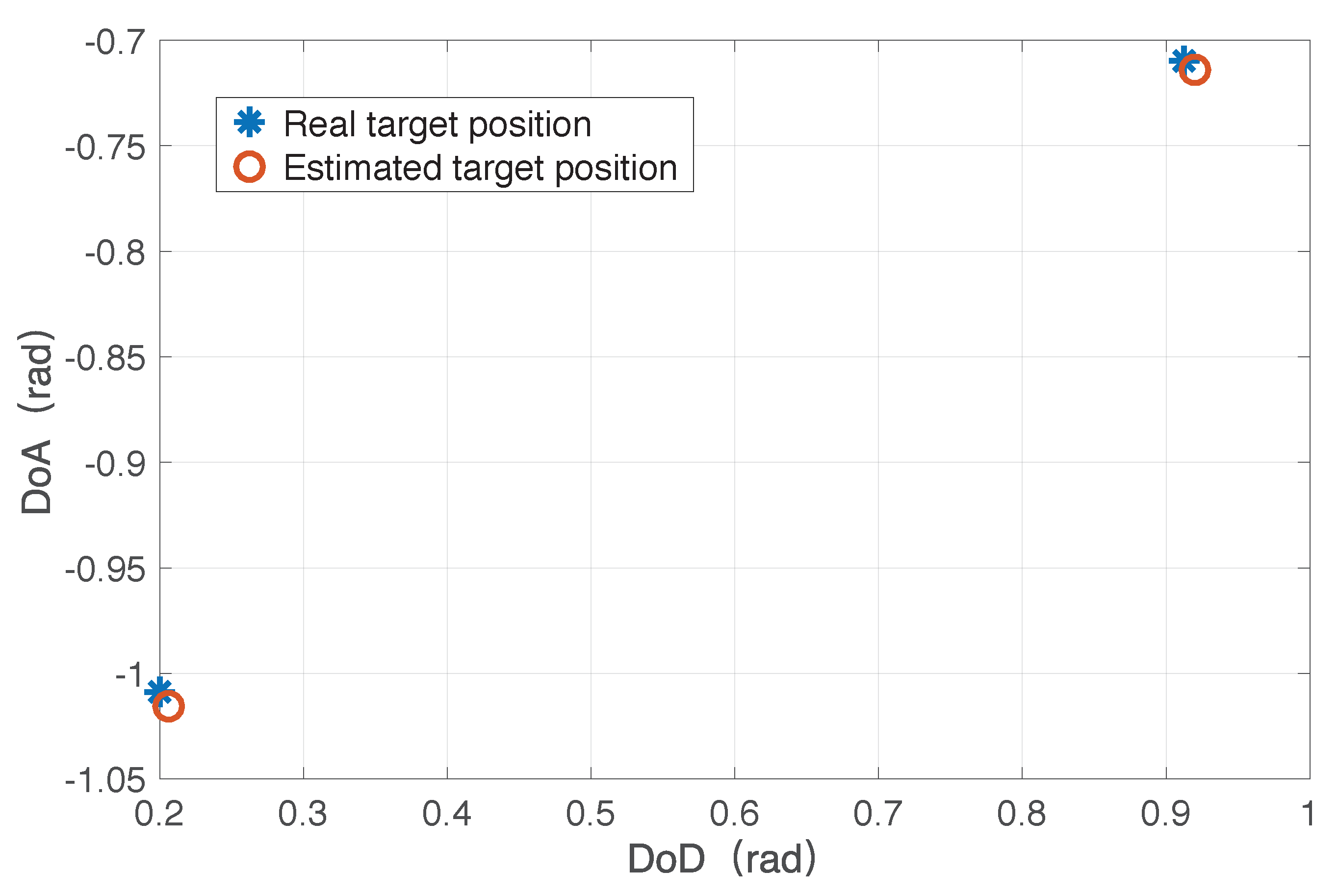
The two targets randomly distribute in the area ${\beta }_k\in [0,\frac{\pi }{2}]$ and ${\alpha }_k\in [-\frac{\pi }{2},0]$, set the numbers of discretized DoD/DoA are both 100, therefore, only two entries are non-zeros, the DoD/DoA estimation problem can be considered as a sparse reconstruction problem, and the OMP method can be used. The simulation results of the OMP estimation method is shown in Figure 3. From Figure 3 we can see that the proposed method can exactly estimate the DoDs/DoAs.

The DoD/DoA estimation performance of two targets is given in Figure 4, and we compare the estimated results with the CRLB derived in this paper. As shown in Figure 4, the RMSEs between simulation and CRLB shows a significant discrepancy in the lower SNR region, and as the SNR increases, the discrepancy can be converged to $0.1$. The discrepancy is mainly caused by the grid mismatch problem with a discrete potential angle space. We can improve it by increasing the discrete grid number. However, it will increase the complexity of the system.

We also give the comparison of the proposed angular estimation positioning system and the traditional GPS. GPS is a wireless navigation system that is positioned by navigation satellites. It consists of space, ground monitoring and user receivers. It can achieve omnipotence (marine, terrestrial, aerospace, aerospace), global, all-weather, continuous and real-time navigation and positioning capabilities provide precise position and speed information. It is one of the navigation systems suitable for port AGV applications.

The AGV positioning geometry is shown in Figure 5. One of the two satellite detectors is used as the coordinate origin $(0,0)$. The distance between the two detectors is L, and the coordinates of the other detector are $(L,0)$. Assuming that the coordinates of the AGV are (x, y), the angles of the AGV signals received by the two satellite detectors can be estimated as $\alpha$ and $\beta$ by the spatial spectrum algorithm. Then, the coordinates of the AGV can be obtained by the following geometric relations

$$\begin{array}{cc}\hfill x& =\frac{Ltan\alpha }{tan\alpha -tan\beta },\hfill \end{array}$$

(28)

$$\begin{array}{cc}\hfill y& =\frac{L}{tan\alpha -tan\beta }.\hfill \end{array}$$

(29)

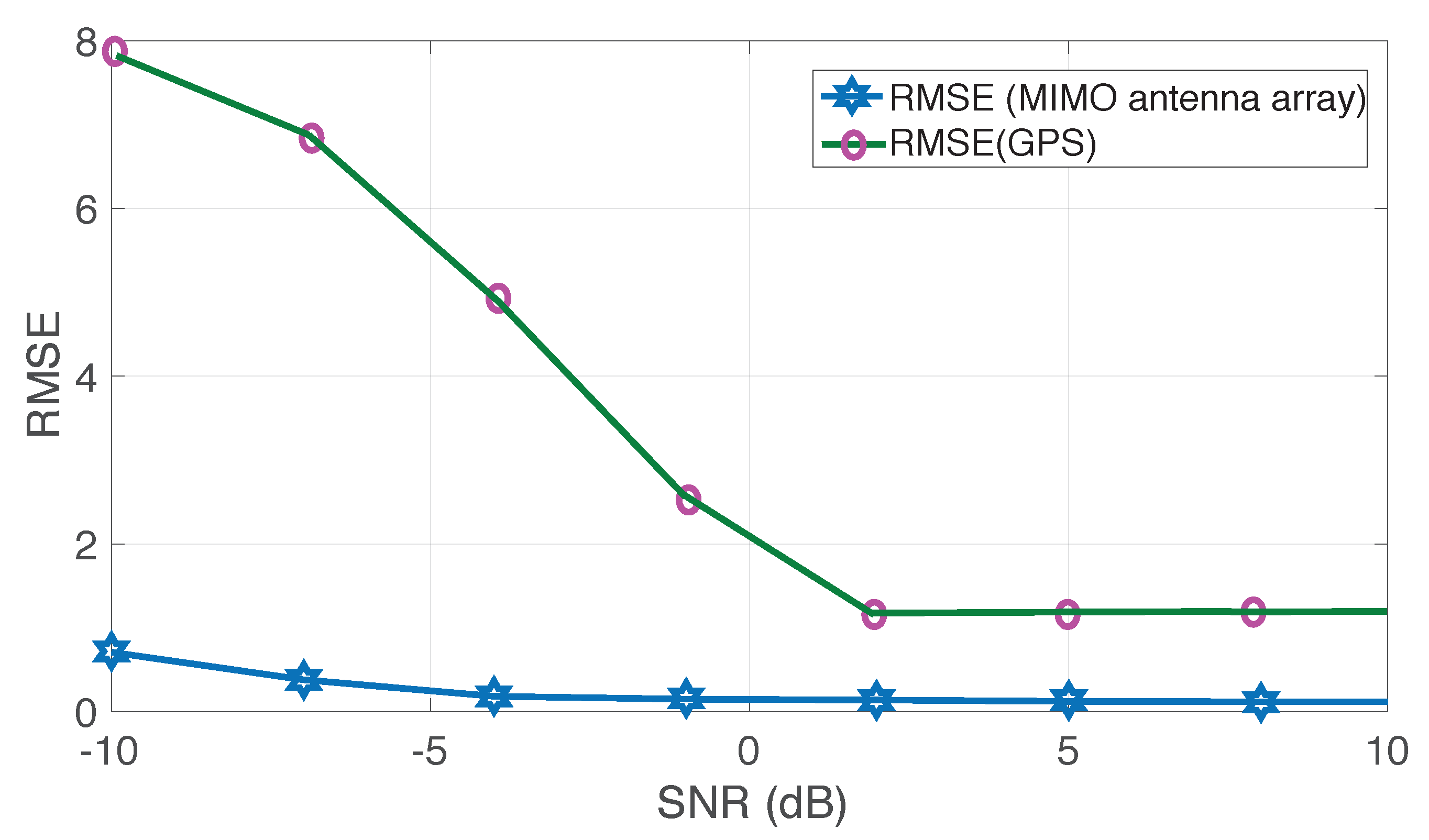
From Equations (28) and (29), we can obtain the AGV $x-y$ coordinate, and the angle can be derived directly. Figure 6 shows the RMSE of both the proposed MIMO antenna positioning method and GPS method, where the SNR of the received GPS signal is the equivalent value after despreaded and the actual SNR of GPS signal is 30 dB lower than that. Additionally, the estimation performance of the proposed method and GPS is shown in Figure 7, we can see that the proposed CS-based positioning method outperforms the traditional GPS method.

7. Conclusions

This paper utilizes the antenna array to acquire the arrival angle information of the transponder signal reaching each antenna, thereby obtaining the position information of the transponder and performing the AGV positioning by using the relative position of the transponder and the AGV. According to the method provided by the present invention, high-precision positioning of the AGV can be realized in an outdoor environment where there are many obstacles such as ports and docks. Compared with the GPS, the positioning method can ignore the influence of obstacles on signal propagation, the system structure can be simplified and the cost can be reduced.

References

- Le-Anh, T.; De Koster, M.B.M. A review of design and control of automated guided vehicle systems. Eur. J. Oper. Res. 2006, 171, 1–23. [Google Scholar] [CrossRef] [Green Version]
- Lei Wang, J.; Shu, T.; Kumagai, M. A 3D scanning laser rangefinder and its application to an autonomous guided vehicle. In Proceedings of the IEEE Vehicular Technology Conference, Boston, MA, USA, 24–28 September 2000; pp. 331–335. [Google Scholar]
- Li, J.; Stoica, P. MIMO radar with colocated antennas. IEEE Signal Process. Mag. 2007, 24, 106–114. [Google Scholar] [CrossRef]
- Davis, M.; Showman, G.; Lanterman, A. Coherent MIMO radar: The phased array and orthogonal waveforms. IEEE Aerosp. Electron. Syst. Mag. 2014, 29, 76–91. [Google Scholar] [CrossRef]
- Chen, Z.; Cao, Z.; He, X.; Jin, Y.; Li, J.; Chen, P. DoA and DoD Estimation and Hybrid Beamforming for Radar-Aided mmWave MIMO Vehicular Communication Systems. Electronics 2018, 3, 40. [Google Scholar] [CrossRef]
- Chen, P.; Wu, L.; Qi, C. Waveform optimization for target scattering coefficients estimation under detection and peak-to-average power ratio constraints in cognitive radar. Circ. Syst. Signal Process. 2016, 35, 163–184. [Google Scholar] [CrossRef]
- Chen, P.; Wu, L. Coding matrix optimization in cognitive radar system with EBPSK-based MCPC signal. J. Electromagn. Waves Appl. 2015, 29, 1497–1507. [Google Scholar] [CrossRef]
- Skolnik, M. Radar Handbook, 3rd ed.; McGraw-Hill: New York, NY, USA, 2008. [Google Scholar]
- Lemma, A.N.; van der Veen, A.; Deprettere, E.F. Analysis of joint angle-frequency estimation using ESPRIT. IEEE Trans. Signal Process. 2003, 51, 1264–1283. [Google Scholar] [CrossRef] [Green Version]
- Chen, Z.; Chen, P.; Li, J.; Miao, P. Non-orthogonal multi-carrier MIMO communication system using M-ary efficient modulation. Digit. Signal Process. 2018, 76, 14–21. [Google Scholar] [CrossRef]
- Zamani, H.; Zayyani, H.; Marvasti, F. An iterative dictionary learning-based algorithm for DOA estimation. IEEE Commun. Lett. 2016, 20, 1784–1787. [Google Scholar] [CrossRef]
- Chen, Z.; Wu, L.; Chen, P. Efficient modulation and demodulation methods for multi-carrier communication. IET Commun. 2016, 10, 567–576. [Google Scholar] [CrossRef]
- Petropulu, A.P.; Poor, H.V. Measurement matrix design for compressive sensing–based MIMO radar. IEEE Trans. Signal Process. 2011, 59, 5338–5352. [Google Scholar]
- Donoho, D.L. Compressed sensing. IEEE Trans. Inf. Theory 2006, 52, 1289–1306. [Google Scholar] [CrossRef]
- Candes, E.J.; Wakin, M.B. An Introduction To Compressive Sampling. IEEE Signal Process. Mag. 2008, 25, 21–30. [Google Scholar] [CrossRef]
- Donoho, D.L.; Tsaig, Y.; Drori, I.; Starck, J. Sparse Solution of Underdetermined Systems of Linear Equations by Stagewise Orthogonal Matching Pursuit. IEEE Trans. Inf. Theory 2012, 58, 1094–1121. [Google Scholar] [CrossRef]
- Massa, A.; Rocca, P.; Oliveri, G. Compressive Sensing in Electromagnetics–A Review. IEEE Antennas Propag. Mag. 2015, 57, 224–238. [Google Scholar] [CrossRef]
- Baraniuk, R. Compressive sensing. IEEE Signal Process. Mag. 2007, 24, 118–121. [Google Scholar] [CrossRef]
- Yao, Y.; Petropulu, A.P.; Poor, H.V. MIMO radar using compressive sampling. IEEE J. Sel. Areas Signal Process. 2010, 4, 146–163. [Google Scholar]
- Zhao, T.; Peng, Y.; Nehorai, A. Joint sparse recovery method for compressed sensing with structured dictionary mismatches. IEEE Trans. Signal Process. 2014, 62, 4997–5008. [Google Scholar]
- Fishler, E.; Haimovich, A.; Blum, R.S.; Cimini, L.J.; Chizhik, D.; Valenzuela, R.A. Spatial diversity in radars-models and detection performance. IEEE Trans. Signal Process. 2006, 54, 823–838. [Google Scholar] [CrossRef]
- Fishler, E.; Haimovich, A.; Blum, R.; Chizhik, D.; Cimini, L.; Valenzuela, R. MIMO radar: An idea whose time has come. In Proceedings of the IEEE Radar Conference, Philadelphia, PA, USA, 26–29 April 2004; pp. 71–78. [Google Scholar]
- Yang, Z.; Xie, L. Exact joint sparse frequency recovery via optimization methods. IEEE Trans. Signal Process. 2016, 64, 5145–5157. [Google Scholar] [CrossRef]
- Chen, P.; Qi, C.; Wu, L.; Wang, X. Estimation of Extended Targets Based on Compressed Sensing in Cognitive Radar System. IEEE Trans. Veh. Technol. 2017, 66, 941–951. [Google Scholar] [CrossRef]
- Khwaja, A.S.; Cetin, M. Compressed Sensing ISAR Reconstruction Considering Highly Maneuvering Motion. Electronics 2017, 6, 21. [Google Scholar] [CrossRef]
- Tropp, J.A.; Gilbert, A.C. Signal recovery from random measurements via orthogonal matching pursuit. IEEE Trans. Inf. Theory 2007, 53, 4655–4666. [Google Scholar] [CrossRef]
- Chen, P.; Zheng, L.; Wang, X.; Li, H.; Wu, L. Moving target detection using colocated MIMO radar on multiple distributed moving platforms. IEEE Trans. Signal Process. 2017, 65, 4670–4683. [Google Scholar] [CrossRef]
- Zheng, L.; Wang, X. Super-Resolution Delay-Doppler Estimation for OFDM Passive Radar. IEEE Trans. Signal Process. 2017, 65, 2197–2210. [Google Scholar] [CrossRef]
- Davenport, M.; Wakin, M. Analysis of orthogonal matching pursuit using the restricted isometry property. IEEE Trans. Inf. Theory 2010, 56, 4395–4401. [Google Scholar] [CrossRef]
- Pinchera, D.; Migliore, M.D.; Lucido, M.; Schettino, F.; Panariello, G. A Compressive-Sensing Inspired Alternate Projection Algorithm for Sparse Array Synthesis. Electronics 2018, 6, 3. [Google Scholar] [CrossRef]
- Chen, P.; Qi, C.; Wu, L. Antenna placement optimisation for compressed sensing-based distributed MIMO radar. IET Radar Sonar Navig. 2017, 11, 285–293. [Google Scholar] [CrossRef]
- Chen, Z.; Chen, P. Compressed sensing-based DOA and DOD estimation in bistatic co-prime MIMO arrays. In Proceedings of the 2017 IEEE Conference on Antenna Measurements & Applications (CAMA), Ibaraki, Japan, 4–6 December 2017; pp. 297–300. [Google Scholar]
- Gogineni, S.; Nehorai, A. Target estimation using sparse modeling for distributed MIMO radar. IEEE Trans. Signal Process. 2011, 59, 5315–5325. [Google Scholar] [CrossRef]
- Beckmann, P. Statistical distribution of the amplitude and phase of a multiply scattered field. J. Res. Natl. Bur. Stand. 1962, 660, 231–240. [Google Scholar] [CrossRef]
Figure 1.
AGV with an antenna frame for track guiding.
Figure 2.
System model of the MIMO antenna for AGV positioning.
Figure 3.
The estimated and the real targets position.
Figure 4.
The 3D positioning error map of GPS.
Figure 5.
Geometry relationship of AGV positioning via GPS.
Figure 6.
RMSE as a function of SNR with different positioning method.
Figure 7.
The estimation performance of the proposed method and GPS.
© 2018 by the authors. Licensee MDPI, Basel, Switzerland. This article is an open access article distributed under the terms and conditions of the Creative Commons Attribution (CC BY) license (http://creativecommons.org/licenses/by/4.0/).
Share and Cite
MDPI and ACS Style
Chen, Z.; He, X.; Cao, Z.; Jin, Y.; Li, J. Position Estimation of Automatic-Guided Vehicle Based on MIMO Antenna Array. Electronics 2018, 7, 193. https://doi.org/10.3390/electronics7090193
AMA Style
Chen Z, He X, Cao Z, Jin Y, Li J. Position Estimation of Automatic-Guided Vehicle Based on MIMO Antenna Array. Electronics. 2018; 7(9):193. https://doi.org/10.3390/electronics7090193
Chicago/Turabian StyleChen, Zhimin, Xinyi He, Zhenxin Cao, Yi Jin, and Jingchao Li. 2018. "Position Estimation of Automatic-Guided Vehicle Based on MIMO Antenna Array" Electronics 7, no. 9: 193. https://doi.org/10.3390/electronics7090193
Note that from the first issue of 2016, this journal uses article numbers instead of page numbers. See further details here.