

Machine Learning Based Fast QTMTT Partitioning Strategy for VVenC Encoder in Intra Coding

1
IETR, UMR CNRS 6164, Electronics and Computer Engineering Department, INSA Rennes, University of Rennes, 35000 Rennes, France
2
Laboratory of Intelligent Systems, Geo-Resources and Renewable Energies, Faculty of Sciences and Technologies, Sidi Mohamed Ben Abdellah University, Fez 30000, Morocco
3
Laboratory of Intelligent Systems, Geo-Resources and Renewable Energies, National School of Applied Sciences, Sidi Mohamed Ben Abdellah University, Fez 30000, Morocco
*
Author to whom correspondence should be addressed.
Electronics 2023, 12(6), 1338; https://doi.org/10.3390/electronics12061338
Submission received: 31 January 2023
/
Revised: 4 March 2023
/
Accepted: 9 March 2023
/
Published: 11 March 2023
(This article belongs to the Special Issue Video Coding, Processing, and Delivery for Future Applications)
Abstract
:The newest video compression standard, Versatile Video Coding (VVC), was finalized in July 2020 by the Joint Video Experts Team (JVET). Its main goal is to reduce the bitrate by 50% over its predecessor video coding standard, the High Efficiency Video Coding (HEVC). Due to the new advanced tools and features included in VVC, it actually provides high coding performances—for instance, the Quad Tree with nested Multi-Type Tree (QTMTT) involved in the partitioning block. Furthermore, VVC introduces various techniques that allow for superior performance compared to HEVC, but with an increase in the computational complexity. To tackle this complexity, a fast Coding Unit partition algorithm based on machine learning for the intra configuration in VVC is proposed in this work. The proposed algorithm is formed by five binary Light Gradient Boosting Machine (LightGBM) classifiers, which can directly predict the most probable split mode for each coding unit without passing through the exhaustive process known as Rate Distortion Optimization (RDO). These LightGBM classifiers were offline trained on a large dataset; then, they were embedded on the optimized implementation of VVC known as VVenC. The results of our experiment show that our proposed approach has good trade-offs in terms of time-saving and coding efficiency. Depending on the preset chosen, our approach achieves an average time savings of 30.21% to 82.46% compared to the VVenC encoder anchor, and a Bjøntegaard Delta Bitrate (BDBR) increase of 0.67% to 3.01%, respectively.
1. Introduction
A recent study was conducted by Cisco shows that, by 2023, video traffic will represent a huge amount of the global Internet traffic [1]. This increase is caused by the high demand on the Ultra High Definition (UHD), High Dynamic Range (HDR), Virtual Reality (VR), Augmented Reality (AR) and 360-degree videos and also the versatility of video applications such as web TV, video on demand, streaming websites, and many other advanced video technologies. These different emerging applications continuously require more efficient video coding techniques than those already adopted in the current video coding standards such as High Efficiency Video Coding (HEVC) [2]. This is why the Versatile Video Coding (VVC) [3] standard introduces many new advanced features to meet these requirements, allowing it to achieve higher coding efficiency, handle various video applications, and support current and emerging video formats. VVC is the new-generation video coding standard developed by the Joint Video Exploration Team (JVET) of the International Telecommunications Union (ITU) and the Moving Picture Experts Group (MPEG). It is intended to be the successor to the current standards and aims to improve compression efficiency by up to 50% while maintaining a high level of video quality over the HEVC standard [3]. Similarly to HEVC, a block-based hybrid video coding scheme was primarily designed for VVC. Additionally, to overcome some limitations of HEVC and enhance VVC coding efficiency further, multiple sophisticated tools were also involved. For instance, in the partitioning block, VVC supports separate trees for Luminance (Luma) and Chrominance (Chroma) partitioning. It also supports larger Coding Tree Unit (CTU) sizes than HEVC by allowing the coding of blocks of 128 × 128 [3]. Moreover, VVC has introduced the new Quad Tree with a nested Multi-Type Tree (QTMTT) scheme, which replaces the previously used Quad Tree structure of HEVC. Another major advancement in the VVC standard is related to the intra-frame prediction. The Intra prediction takes full advantage of the spatial redundancy within the same frame to predict a Coding Unit (CU). This predicted sample is based on the neighboring samples in the left and above CUs that have already been encoded. Moreover, the intra-frame prediction in VVC utilizes significantly more modes for prediction compared to HEVC, which only supported 33 angular modes in addition to Planar and DC modes [3]. VVC has expanded the number of angular modes to 65 angular and wide angular modes, while still maintaining the DC and Planar modes. Furthermore, new prediction techniques for intra-frame coding were added in VVC. Among them, the adoption of Intra Sub-Partition (ISP), which divides the CU Luma component into two or four sub-partitions vertically or horizontally and shares the coding mode information while separating the prediction and transform processes. Another intra-frame technique, called Multiple Reference Line (MRL), has been added to allow the prediction of Luma samples from non-adjacent reference lines that can be two or three lines away from the current block. Other techniques, such as Wide-Angle Intra Prediction (WAIP), Cross-Component Linear Model (CCLM), and Matrix-based Intra Prediction (MIP), have also been included in VVC. The Transformation and Quantization block in VVC was designed similarly to HEVC. In addition, VVC introduced a new Multi Transform Selection (MTS) block by supporting more separable trigonometrical transform types in addition to those already used in HEVC. It added to the DCT-2, two new types of sine and cosine transform (DST-7 and DCT-8). The Low-Frequency Non-Separable Transform (LFNST) was also introduced in this video coding standard [3]. VVC incorporates additional features and tools to improve its coding efficiency, at the cost of a high computational complexity. As a result, when compared to HEVC, a greater number of coding tools are supported in VVC, though for an optimized encoder, evaluating all possible choices per each tool is typically not practical because of the high cost of the search space.
Many previous works in the literature are highly active to overcome the VVC computational complexity. Some of them focused on hardware implementations [4,5,6,7]. While others aim to reduce this complexity by using statistical- and heuristic-based approaches, such as [8,9,10], or algorithmic optimization, by introducing Machine Learning (ML) and Deep Learning (DL) based approaches, such as [11,12,13,14,15].
Machine learning and deep learning have shown a significant efficiency in various domains, since they can be used to address a wide range of complex problems. In the field of medical diagnosis, machine learning algorithms have been used to analyze medical images and detect anomalies, leading to improved diagnosis and better patient outcomes [16,17]. Similarly, deep learning has been used in the renewable energy sector to optimize energy production and improve solar panel efficiency, which can lead to cost savings and a reduced environmental impact [18]. The efficiency of ML and DL in these and other domains depends on various factors such as data quality and quantity, model accuracy, and specific requirements of each domain. Nonetheless, with the right data and models, ML and DL can greatly improve efficiency and increase accuracy in a wide range of applications. In this context, due to the increasing demand on video applications, it is crucial to find ways to reduce the computational complexity of video coding standards while preserving a high coding efficiency. Machine learning presents itself as a promising solution in this scenario, as it has the potential to significantly reduce the computational effort without having a huge impact on the coding efficiency.
Among the various machine learning techniques, Light Gradient Boosting Machine (LightGBM) has been proven to be a highly effective and versatile approach. This technique has been used in a broad range of applications and has demonstrated remarkable results [19]. LightGBM is based on Decision Tree (DT) classifiers and is designed to be hardware-friendly, making it ideal for use in battery-powered devices commonly used in video applications. Furthermore, LightGBM provides superior customization compared to other traditional machine learning techniques, such as Support Vector Machine (SVM), Decision Tree (DT), and Random Forest (RF) [19]. This is due to the combination of gradient descent and boosting techniques that LightGBM employs, which offers a large set of adjustable hyper-parameters that can be optimized for the specific needs of the application. Thus, LightGBM demonstrated an outstanding results in various cases which make it an ideal choice for video coding applications [13].
In this particular case, our contributions rely on proposing a new approach to reduce the complexity of VVC encoder targeting real-time processing by optimizing the CU partitioning of the VVC encoder in intra configuration. In order to achieve this goal, we combined the use of an optimized implementation of VVC by selecting the VVenC encoder developed by The Fraunhofer Heinrich Hertz Institute (HHI) [20], and the use of an efficient machine learning algorithm through the use of LightGBM [21], which offers a reduced inference time. The LightGBM models were trained using a dataset generated by the VVenC encoder by extracting features during the encoding process. In addition, instead of the usually used multiclassification strategy, a new method based on five binary classifiers is introduced in order to handle the classification problem. Moreover, to tackle the problem of misclassification, we used the concept of risk intervals, which leads to improving the classification performances. This way results in a noticeable decrease in the computational complexity with a slight and acceptable increase in the BDBR loss. The main target is the design of a real-time encoder with multiple trade-off points between rate distortion performances and time-saving. We also proposed a new preset that is designed to provide a good balance between the encoding time and the coding efficiency, making it an attractive option for real-time video encoding applications. It should also be noted that all the mentioned state-of-the-art works were integrated into the VVC Test Model (VTM) reference software [22], whereas our approach has been integrated into the VVenC encoder. This can help to validate and demonstrate the effectiveness of our approach, and can contribute to the development of new and improved video encoding techniques.
The remainder of this paper is organized as follows: Section 2 presents the VVenC encoder, the partitioning block in VVC and a review of the state-of-the-art works focusing on the complexity reduction of this block. Section 3 describes the proposed method to reduce the complexity of the CU partitioning in VVC. In Section 4, experimental results are shown and compared to the literature results. Finally, the paper is concluded in Section 5.
2. Background and Related Works
2.1. VVenC: An Open and Optimized Implementation of VVC Encoder
Since the standardization of VVC, JVET supplies a VVC Test Model software reference called VTM [22]. It is usually used as the reference software to evaluate the proposed techniques dedicated to the complexity reduction. Furthermore, just after the finalization of VVC standard, the Fraunhofer HHI presented a project to develop an encoder based on VTM software with the purpose of providing a real-world encoder known as VVenC [20]. VVenC can be defined as an open optimized implementation of VVC including all VTM’s performance at shorter runtimes. Moreover, it presents real-world encoder features such as single-pass and two-pass rate control, and an efficient multi-threading for a further speedup. Based on VTM and written in C++, the VVenC software has been optimized with a new design to reduce performance bottlenecks, enhanced SIMD optimization, faster encoder search algorithms, and multi-threading support to take full advantage of parallel processing. In addition, VVenC offers practical encoding features such as frame-level bitrate control and visually optimized encoding to support a dynamic, quick, as well as an easy-to-use video encoding solution for the VVC standard. Thus, VVenC is more optimized for a Random Access (RA) use case and for high resolution videos [23]. Additionally, two standalone encoder executables are provided, known as vvencapp and vvencFFapp. The first executable, vvencapp, is a simple application optimized for ease of use and only provides basic options. The second one, vvencFFapp, is a full-featured encoder application with a VTM style interface, allowing for the specification of more options and parameters’ configuration.
VVenC allows users to select from different speed presets to find the best trade-off between encoding efficiency and speed. The five speed presets available are Slower, Slow, Medium, Fast and Faster [23]. The Slower preset offers a higher coding efficiency, but it takes more time to encode a video. The Slow preset, on the other hand, takes less time for encoding compared to the Slower, at the cost of a decreased coding efficiency. The Medium preset offers a balance between encoding speed and output quality. The Fast preset, in contrast, prioritizes speed over quality and thus it takes less time to encode a video but produces a lower image quality. The Faster preset takes the shortest amount of time to encode with the lowest coding efficiency. Thus, users can select the most appropriate preset based on their specific requirements and the trade-off between quality and speed that is acceptable for their applications. The VVenC analysis in [24] confirm that these presets are selected based on whether the target is to achieve a high visual quality or a reduced encoding time as well as they show a consistent behavior for random-access encoding.
2.2. The Partitioning Block in VVC
Like the vast majority of video encoders, VVC includes five main steps [3]: The partitioning block that divides the frame into smaller blocks to be encoded, the prediction block, for either intra- or inter-frame prediction, the transform and quantization, and the entropy coding, as illustrated in Figure 1.
Concerning the partitioning block in VVC, each frame is initially divided into one or more tile rows and one or more tile columns. A tile is a group of Coding Tree Units (CTUs) that cover a rectangular area in a frame. This latter is made up of one or three Coding Tree Blocks (CTBs), depending on whether the video signal is a monochrome signal or has three color components. In addition, VVC supports separated trees for both Luma and Chroma partitioning [3].
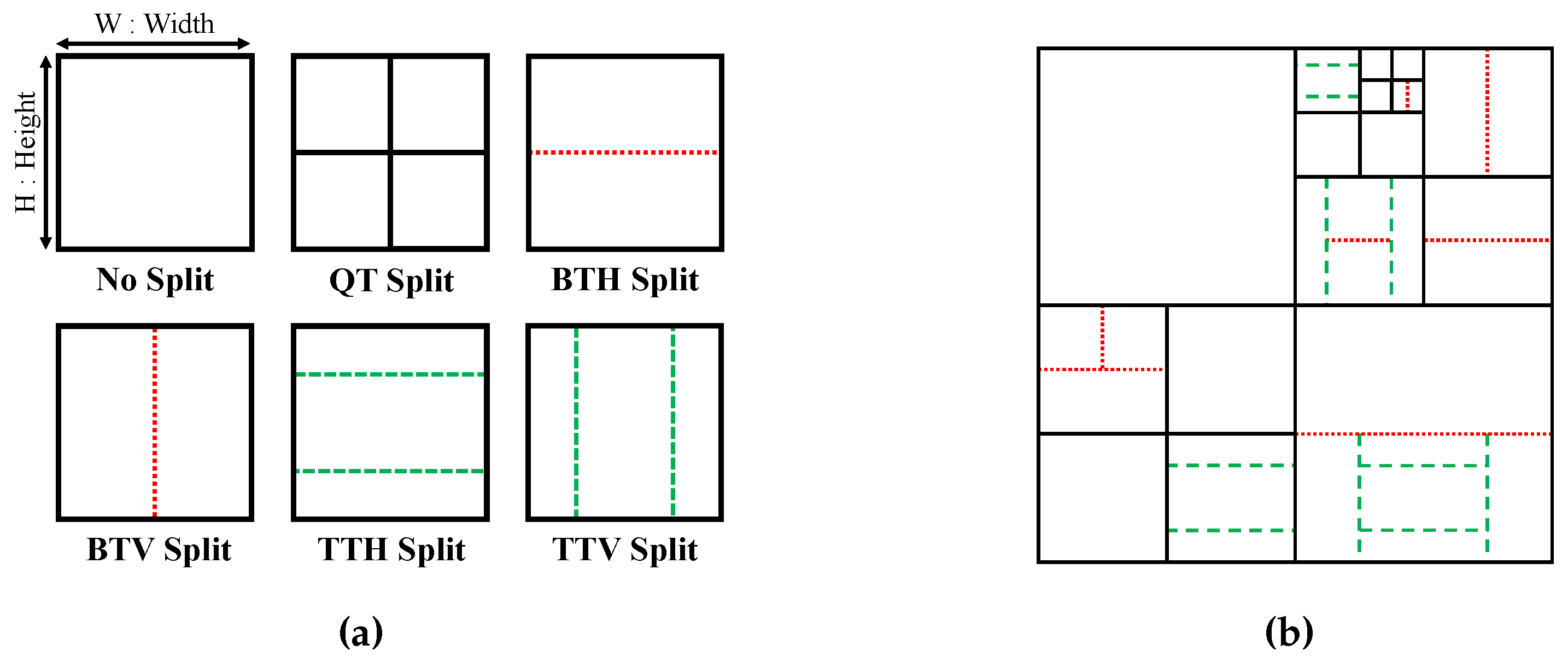
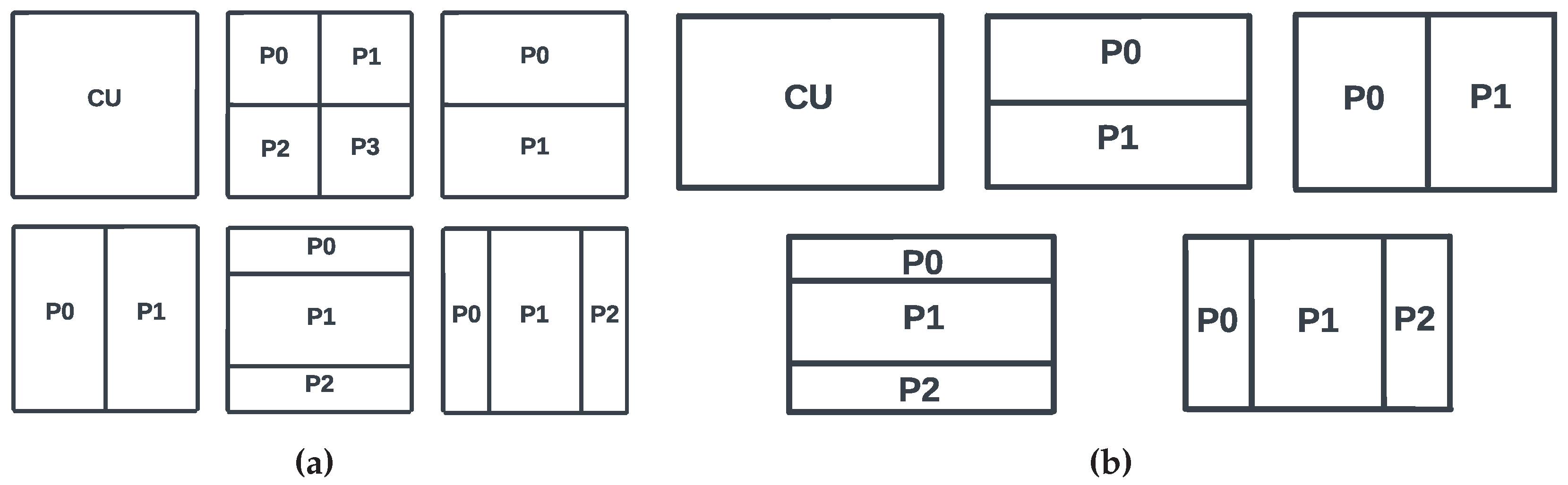
As a result, a picture is segmented into equal-sized blocks called CTU, with a maximum size of 128 × 128 pixels. Then, each frame is processed from top left to bottom right in a raster scan order. Furthermore, in a low level, each CTU is recursively subdivided into smaller blocks, either square or rectangular shapes, called Coding Units (CUs); using the recursive quad tree and finer mode splits binary and ternary tree in both directions, horizontal and vertical. This leads to six possible split modes, including: No Split (NS), Quad Tree (QT), Binary Tree Horizontal (BTH), Binary Tree Vertical (BTV), Ternary Tree Horizontal (TTH) and Ternary Tree Vertical (TTV), as illustrated in Figure 2a.
In the QTMTT scheme, if a CU is assigned the NS mode, it retains its original size and the coding process begins. If a CU of size W × H (W: Width, H: Height) is defined as a QT split, it is divided into four equal sub-CUs of size W/2 × H/2. For a CU with a BTH split mode, it is divided into two sub-CUs of size W × H/2 or W/2 × H for a BTV split mode. For a CU with a TT split mode, it is divided into three sub-CUs. For TTH, the first sub-CU has a size of H/4 × W, the middle one has a size of H/2 × W, and the last one has a size of H/4 × W. However, for a TTV split, the first sub-CU has a size of H × W/4, the second one has a size of H × W/2, and the third one has a size of H × W/4. These different split modes result in a partitioning scheme of six possible modes, as illustrated in Figure 2a, while Figure 2b represents an example of CTU division using the QTMTT scheme. During the encoding process, VVC uses the Rate Distortion Optimization (RDO) process, which is involved in comparing multiple coding options for each coding unit. These coding options include different coding and prediction modes, among others. The goal of the RDO process is to find the optimal coding option that provides the best trade-off between rate and distortion for each coding unit in video frames. Thus, VVC uses the RDO process to evaluate the six options available in the QTMTT scheme in order to minimize the distortion of the reconstructed video while keeping the bitrate low. The best CTU partitioning structure is the one leading to the lowest Rate Distortion cost () [25] calculated by Equation (1):
where D stands for the calculated distortion between the original and predicted blocks, B denotes the cost in bits of a specific mode, multiplied by , which is the Lagrange multiplier.
VVC added some constraints to limit the larger number of possible split combinations. Therefore, each CU split mode has to necessarily respect the constraints of the maximum and minimum sizes of CUs as mentioned in the VTM draft [22]. In fact, in All Intra configuration, VVC forces a CTU of 128 × 128 to be divided into four sub-CUs following the QT split. Then, for each 64 × 64 CU, VVC checks whether it can be divided into four sub-CUs following the QT split or to keep the original CU size. Table 1 shows all the possible splits corresponding to each CU size in the All Intra configuration.
In addition to the constraints on CU size, several other limitations must be respected. For example, a QT split is no longer allowed after a BT or a TT split. Thus, Figure 2b shows a possible CTUs partitioning with the QT, BT, and TT splits combination performed by the QTMTT scheme included in VVC.
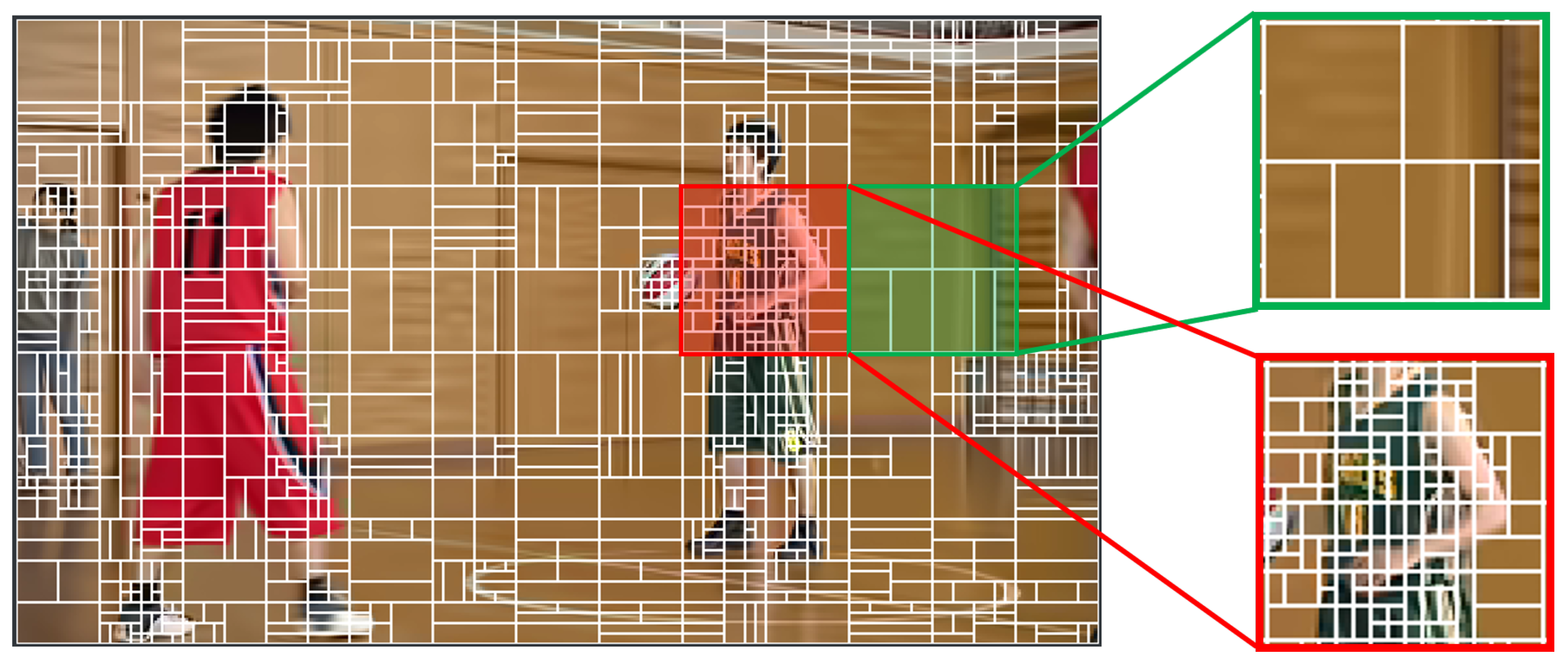
Figure 3 illustrates the first frame of BasketballPass video sequence in the Common Test Conditions (CTC) sequences [26]. This frame was encoded using the VVenC encoder under the All Intra configuration, with a Quantization Parameter (QP) of 37. The smooth areas of the image tend to have fewer details, so larger blocks can be used to encode them as shown in the green square. For areas with complex texture, smaller blocks are used to better capture the details of the image. This allows the encoder to more efficiently compress the data in the video. It is critical here to highlight that there are additional factors that influence coding efficiency and encoding time—for instance, the QP value as well as the depth of QT and MTT splits. Overall, the RDO process is a computationally intensive process, as it requires evaluating the RD cost for a large number of possible CU partitions. However, it is a highly effective technique for achieving high-quality video compression, as it enables the encoder to select the optimal coding mode for each CU based on its content and complexity.
2.3. Related Works
One of the key features of VVC is the use of the RDO process, which allows for an efficient decision-making by selecting the optimal configuration choices at each level of the coding process such as partitioning, intra/inter prediction, transform, etc. However, this process can increase the computational complexity of the encoder since it requires testing all possible coding modes for each coding block before selecting the optimal one. To address this issue, various optimization techniques were proposed, including early termination and fast algorithms to reduce the number of candidate modes to be tested and speed up the RDO process.
A study by Tissier et al. [27] has shown that there are several opportunities for reducing the computational complexity of VVC in various modules. They encoded the different CTC sequences using VTM 3.0 in All Intra configuration mode, and they save the ground truth values for the three block (Partitioning, Transform, Intra-prediction). These parameters were used as input for the second test, where they directly use the optimal choices without passing by the RDO process. It was confirmed by this study that around 97% in encoding time could be saved if the optimal split mode in the partitioning block could be directly predicted, which has a great potential for complexity reduction.
In [9], the authors proposed an early termination algorithm to skip unnecessary CU split modes, by using a directional gradient that can directly decide either to Horizontally or Vertically split the current block for both binary and ternary modes. This algorithm can save around 52% in encoding time with a BDBR degradation of 1.2% when compared to the reference software VTM 5.0.
In [28], Fu et al. proposed a fast CU partitioning algorithm that incorporates two early skipping methods. The first method skips vertical splits (BTV and TTV) early, and the second one skips horizontal ternary splits (TTH) early. This approach was integrated into VTM 1.0, and it resulted in an average time savings of 45% with an increase in BDBR of about 1.02%.
With the emergence and the excellent performances of Machine Learning (ML), many researchers have introduced several ML algorithms to the video compression field. For instance, Tissier et al. proposed a two-stage learning-based technique in [11]. This method was implemented in VTM 10.2, and it uses a Convolutional Neural Network (CNN) to predict the spatial features of the input block by employing a vector of probabilities that describes the partition at each 4 × 4 edge. After that, a Decision Tree (DT) model is used to predict the most probable splits at each block using this vector of spatial features. The RDO process then only processes the N most probable splits based on this prediction. Their approach was able to achieve a significant reduction in encoding time of 47.4% and 70.4%, with a BDBR loss of 0.79% and 2.49%, for the top-3 and top-2 configurations, respectively.
Li et al. in [12] proposed a deep learning approach to accelerate the encoding process of the intra-mode in VVC by predicting the CU partition mode. This approach is based on a Multi-Stage Exit (MSE) CNN which takes as input the CTU and then decides at each stage, among others, the most probable split mode according to the CU size. Therefore, they reduced the encoding time from 44.65% to 66.88% with a degradation in BDBR from 1.322% to 3.188%, respectively, over the original VTM 7.0.
Qiuwen et al. in [29] proposed a fast CU partition decision approach based on DenseNet Network, and it was integrated into VTM 10.0. This approach takes a CTU and divides it into four blocks of 64 × 64. These blocks are used as input for a CNN to predict the probability that the boundaries of all the 4 × 4 blocks within each 64 × 64 CU are divided. This method can save around 53.98% of encoding time while increasing the BDBR by 1.80%.
In [30], Hoang et al. proposed a fast CU partition method for intra prediction using an Early-Terminated Hierarchical CNN model to predict the coding unit map, which is also fed into the VVC encoder to early terminate the block partitioning process. In addition, according to experimental results, this method reduced the encoding time by 30.29% with a BDBR increase of 1.39% over the VTM 12.1.
A fast CU partitioning approach for VVC intra coding was also proposed by Zhang et al. [31], where they designed a Global Convolutional Network (GCN) module with a large kernel size convolution, which is able to effectively capture the CU global information and predict the partition mode over the QTMTT structure. With this technique implemented in VTM 10.0, they achieved an encoding time reduction ranging between 51.06% and 61.15% with an increase of the BDBR varying from 0.84% to 1.52%. They also used this method to accelerate VVenC at its slower preset, where they showed that the proposed slower maintains the same average coding performance with a reduced encoding time in comparison with the slow preset original. They also showed that the accelerated VVenC slower decreased the BDBR by 0.25% in comparison with the medium, which resulted in an improved performance and less complexity.
Based on a machine learning algorithm, authors in [13] designed a configurable fast block partitioning for VVC by using LightGBM models to directly predict the CU split without passing through the RDO process. This approach was embedded on VTM 10.0, and it can save around 54.20% in encoding time with an increase in BDBR of 1.42%.
A fast coding unit partition decision algorithm is presented by Chen et al. in [14]. This algorithm is based on six Support Vector Machine (SVM) classifiers to select the division directions using some features that are derived from entropy, texture contrast, and Haar-wavelet of the current CU. Experimental results of the comparison with the reference VTM 4.0, show that this method can save around 51.23% of encoding time with a degradation in BDBR by 1.62%.
A two-stage machine learning approach is designed by Quan et al. [15] based on two Random Forest (RF) [32] classifiers integrated into VTM 7.0, where the CUs are initially separated into three types named: simple, fuzzy, and complex CUs. The first RF classifier is developed to directly find the best division mode for both simple and complex CUs. Another RF classifier is used for fuzzy CUs to predict whether the partition process is terminated or not. This method can save about 57% of encoding time with an increase of 1.21% in BDBR.
In [33], a machine learning-based algorithm is proposed to accelerate the VTM 10.0 encoder, where they use two SVM classifiers to terminate the redundant partitions early. The classifiers were trained to predict the CU partition mode using texture information. The first classifier is used to test if a CU should be split or not, and the second classifier is to predict if the split should be horizontal or vertical. This approach yields a 63.16% reduction in encoding time and a BDBR loss of 2.71%.
A summary of the machine learning based algorithms for CU partitioning block complexity reduction is presented in Table 2 for an easier comparison. These results confirm that CNNs provide better trade-offs, but their hardware implementations’ complexity is still a big challenge, due to the computational requirements and the need of a large number of parameters to achieve a better accuracy. Additionally, it can be clearly seen that other ML models such as RF in [15] and LightGBM in [13] outperform other ML models in this use case when applied to the VTM software.
3. The Proposed Method
In the VVC standard, the RDO process has also been employed in the CU partition process to improve the coding efficiency. It is involved in evaluating all possible split modes to select the optimal one that provides the lowest RD cost, as described in the previous Section 2.2. However, reducing the encoding time while maintaining the coding efficiency can be achieved by skipping certain evaluations in the QTMTT structure. This approach is desirable for optimizing the CU partitioning process and can lead to an improved overall performance.
Since our main goal is to design a real-time encoder, we combined the use of an optimized implementation of VVC known as VVenC [20], and the use of an efficient ML algorithm called LightGBM [21], which is also less complex and simple to be embedded in the encoder compared to some other ML algorithms [21]. LightGBM models were trained to select the most probable split mode of each coding unit, using the features extracted from the pixel domain that provide significant information about the texture complexity of the CU. Furthermore, instead of using only one multi-classifier, the multi-classification problem was divided into a binary classification by introducing five binary classifiers to make the decision. The decision is made using risk intervals for each classifier rather than default thresholds. As a result, the classification performance of the classifiers was improved, as described in the following sections. These LightGBM classifiers were subsequently integrated into the VVenC encoder to directly predict the most probable split mode to pass to the RDO process and skip the evaluation of the remaining modes.
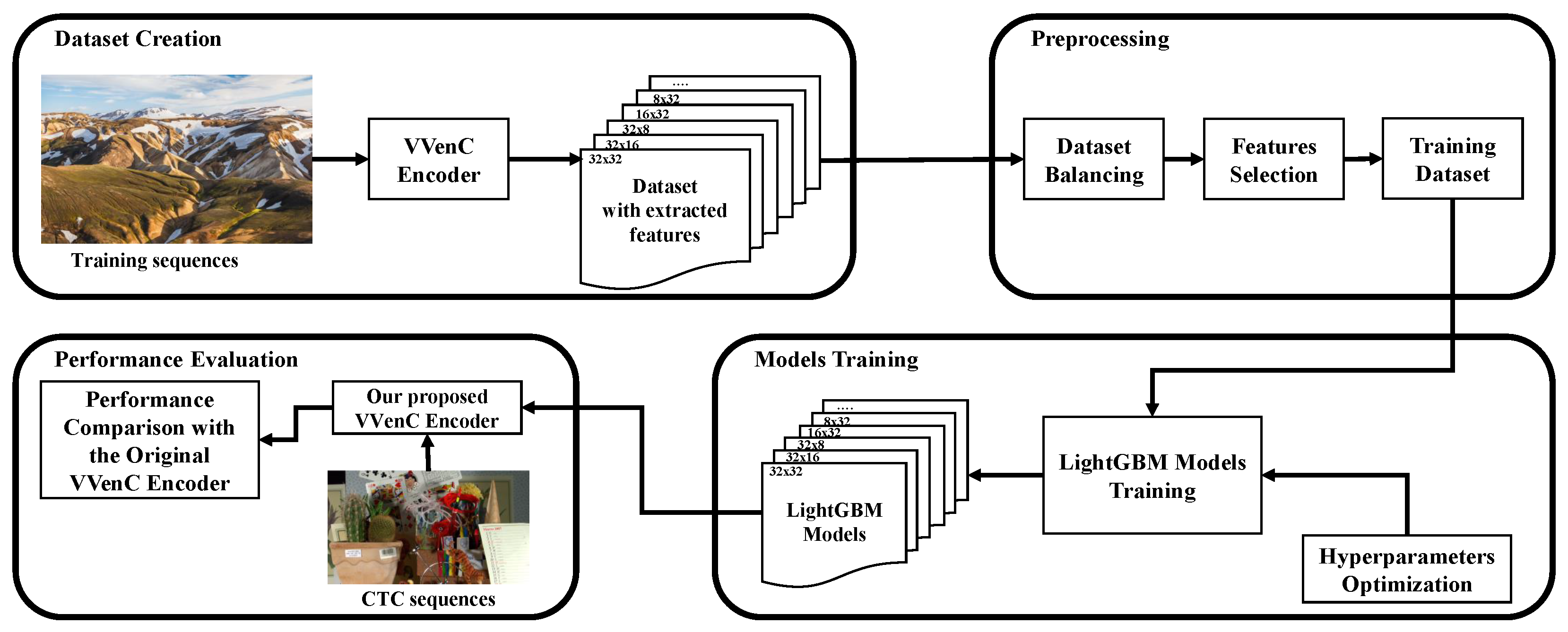
The main stages of our approach are illustrated in Figure 4. First, a set of video sequences was created using different image databases such as Div2k, 4K images, and flickr2k. These video sequences were then encoded using the modified VVenC encoder capable of calculating the CU texture information and other features to generate the dataset of each split mode over the six possible options in the QTMTT scheme, including No split, QT, BTH, BTV, TTH, and TTV. The dataset was preprocessed in the preprocessing stage using dataset balancing and feature mutual information to select the most important features for the training process. In the training stage, the hyper-parameters were optimized using the Optuna tool [34], and then they were used to train our classifiers to be integrated into the VVenC encoder. Finally, our proposed encoder was evaluated according to the Common Test Conditions [26] using the 22 CTC video sequences, and the four values of QP including 22, 27, 32, and 37. The results are presented in the experimental results Section 4.
3.1. Fast CU Partition Decision Structure
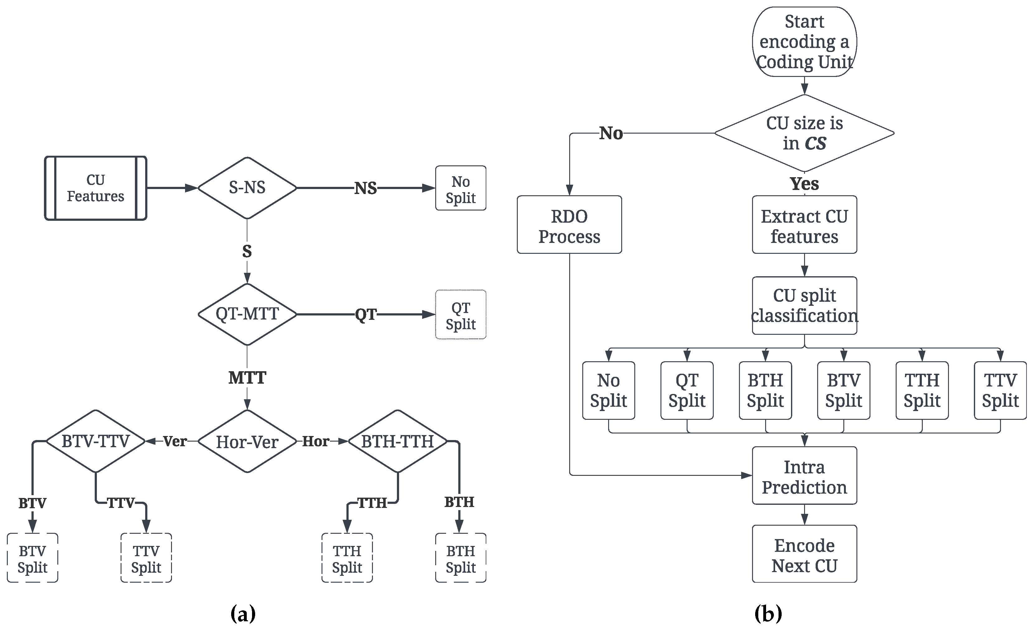
The prediction of the partition that results in the best image quality for each CU while minimizing its RD-cost is the objective of our solution. By ignoring certain split modes, the number that must be checked by the RDO process is reduced. Thus, the selection of the best split mode among the six possible splits already presented in Figure 2a is the problem that must be addressed. As a result, the six-class classification problem has been approached by separating it into five consecutive binary classifiers, as depicted in Figure 5a, rather than building a single LightGBM classifier to handle it directly. This separation affords greater flexibility in the decision structure and allows for the training of each classifier on specific features, resulting in improved classification performance. This new suggested technique investigates eight CU size classes in (CS ), where CS ∈ {32 × 32, 32 × 16, 16 × 32, 16 × 16 32 × 8, 8 × 32, 8 × 16, 16 × 8}. Other CU sizes are processed by the RDO process in the encoder directly as illustrated in Figure 5b.
The five binary classifiers are used in a specific order and they are named according to their function as follows:
- S-NS: It is used to decide whether a block should be divided into smaller sub-blocks or encoded as it is;
- QT-MTT: It is used to decide the type of tree structure used for dividing the CU, it could be QT or Multi Type Tree (BT, TT);
- Hor-Ver: It is used to decide the direction of the split, it could be horizontal or vertical;
- BTH-TTH: It is used to determine whether a BTH or TTH split is the optimal option for a given CU;
- BTV-TTV: It is used to determine whether a BTV or TTV split is the best option for a given CU.
Indeed, after evaluating the intra-frame prediction of the concerned CU sizes, our solution calculates and extracts the coding unit features to feed the LightGBM classifiers. Then, the classification is made following the already presented algorithm in Figure 5a. Subsequently, the most probable split type is selected according to the prediction process detailed in Section 3.4 to be processed by the RDO process. Otherwise, the encoder calls the RDO process to test all possible split types and select the one with the lowest RD-cost. Finally, the CU partitioning process is terminated for the current CU and started for the next one.
3.2. Dataset Creation and Feature Extraction
To enhance and improve the training process of the LightGBM models, a dataset was created for this purpose. As the study focuses on All Intra coding, no temporal relationship between frames is required. Therefore, five public picture databases were selected for the dataset, as described in [11], which are: 4K images, Div2k, jpeg-ai, HDR google, and flickr2k. The images were then down-scaled to generate various resolutions, and finally the pseudo-video sequences were created by combining the images of the same resolution, as shown in Table 3, which presents the number of images per resolution.
The modified VVenC encoder was used to encode the pseudo-video sequences using the Slower preset in order to extract the CU features with the corresponding split mode as labels. For this purpose, various pixel domain features of CUs and sub-CUs were carefully selected, such as the quantization parameter, the horizontal and the vertical gradients, the block pixels mean, the block variance and the sub-blocks’ texture complexity difference. These features were calculated as described in our previous work [35], among these features:
- Quantization Parameter, QP:
- The vertical gradient, GradV:
- The horizontal gradient, GradH:
- The CU Pixels Mean, CUMean:
- The CU Pixels Variance, CUVar:
- The sub-CU’s texture complexity, SCTC:where W and H represent the width and height of the CU or the sub-CU, respectively. denotes the variance of the i sub-CU, obtained by Equation (5). is the average value of the variance of the sub-CUs, corresponding to the split mode noted by j, whereas k denotes the number of sub-CUs parts as indicated in Table 4:
The calculation of these features is performed for the entire CU and all of its sub-CUs parts denoted by . For a square-shaped CU, the features are calculated for the sub-CUs parts as shown in Figure 6a. In the case of a rectangular CU, the features are calculated by evaluating its respective sub-CUs parts, as depicted in Figure 6b.
3.3. LightGBM Models Training
The proposed fast CU partition decision approach uses the LightGBM algorithm which is an open-source machine learning tool that builds a model based on the Gradient Boosting Decision Tree (GBDT) approach [21]. This algorithm is known for its efficiency in training on large datasets while using minimal memory. It incorporates two innovative techniques, Gradient-based One-Side Sampling (GOSS) and Exclusive Feature Bundling (EFB), to enhance performance. GOSS allows LightGBM to train on each tree using only a small portion of the entire dataset, while EFB enables it to handle high-dimensional sparse features more efficiently. In addition, LightGBM supports distributed training, which reduces communication costs, and GPU-accelerated training, which speeds up the training process [21]. It is known for its efficiency and scalability, making it a popular choice for training large models on large datasets. It is also designed to be distributed and efficient, having the ability to handle a large-scale of data with lower memory usage. It has many hyper-parameters that can be tuned to improve the model performance, such as the maximum number of leaves in a tree, the learning rate, the maximum depth of a tree, and the minimum number of samples required at a leaf node, as well as other hyper-parameters that control the fraction of samples and features used for training a single tree [21]. Hyper-parameter tuning is an essential step in optimizing the performance of LightGBM models, and various techniques such as grid search or Bayesian optimization can be used to find the optimal values for these hyper-parameters. In order to optimize our training parameters, we applied the the Tree-structured Parzen Estimator (TPE) algorithm [36] using Optuna tool, which is a Python library for hyper-parameter tuning that supports random search, grid search, and other algorithms [34]. Thus, we estimated the best parameter values as presented in Table 5.
The LightGBM models were trained on a computer with Intel Xeon(R) W-2145 CPU @ 3.70 GHz, NVIDIA GeForce RTX 2080 Ti GPU and 64 GB RAM, using Ubuntu 20.04 LTS as an operating system. We trained our LightGBM classifiers independently for each size of CUs. Then, after obtaining the trained models for the CU sizes, with: CUSize ∈ {32 × 32, 32 × 16, 16 × 32, 16 × 16 32 × 8, 8 × 32, 8 × 16, 16 × 8}, they were integrated into the VVenC encoder according to the proposed flowchart shown in Figure 5b to predict the split mode for CUs during the encoding process.
To evaluate the classification efficiency of our trained classifiers, we measured their performances using the base metrics commonly used for machine learning models evaluation, such as Accuracy, Precision, Recall and F1-score.
Accuracy is defined as the number of accurately classified instance divided by a total number of instances in the dataset. It is calculated as in Equation (7),
where
- TP stands for True Positive, and it represents an instance that is actually positive (i.e., belongs to the class 1), and it is correctly classified as positive by the model;
- TN means True Negative, and it represents an instance that is actually negative (i.e., belongs to the class 0), and it is correctly classified as negative by the model;
- FP means False Positive, and it corresponds to an instance that is actually negative but is incorrectly classified as positive by the model;
- FN means False Negative, and it corresponds to an instance that is actually positive but is incorrectly classified as negative by the model.
Precision is a metric that measures the proportion of true positive predictions among all positive predictions made by a machine learning model. In other words, it measures the model’s ability to correctly identify the positive class. Precision is calculated as in Equation (8),
Recall, also known as sensitivity or true positive rate, is a metric that measures the proportion of true positive instances that are correctly identified by a machine learning model. In other words, it measures the model’s ability to correctly identify the positive class among all positive instances in the dataset. It is calculated as in Equation (9),
By taking both precision and recall into account, the F1 score provides more significant information about the model performance, where a high F1 score indicates that the model is able to achieve both high precision and high recall, while avoiding false positives and false negatives. F1-score is calculated as defined in Equation (10):
Consequently, Table 6 presents the accuracy and F1 score results achieved by each classifier. It is clearly shown that these results are stable, which indicates that our trained models achieved good classification performance.
These results confirm the effectiveness of the classifiers in the prediction of the CU split mode, which could potentially lead to an improved video coding efficiency. Furthermore, in comparison with the LightGBM classifiers used by Saldanha et al. in [13], our classifiers outperform them by achieving better classification performance. Indeed, most of our classifiers achieve an accuracy up to 72%, while some of them reach around 98%.
3.4. Prediction Process and Decision-Making
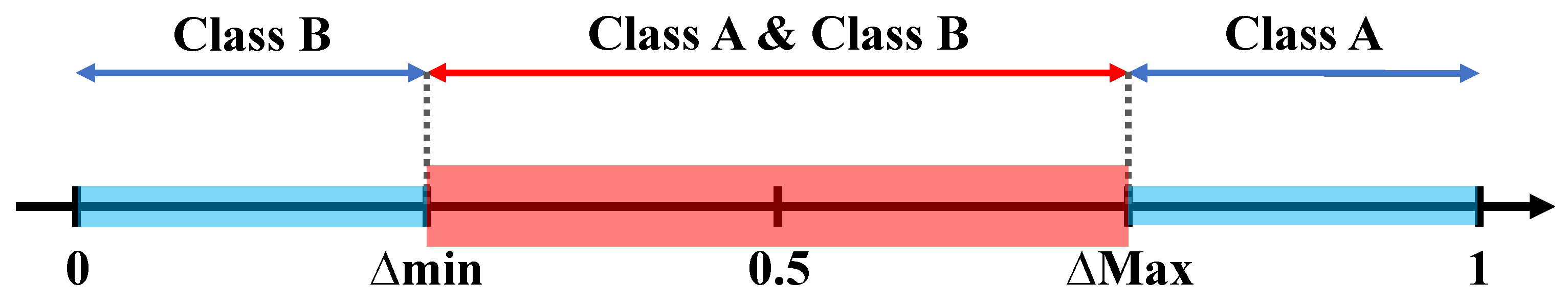
Misclassification is a common problem in classification tasks, where classifiers may incorrectly assign an instance to a class [35]. One reason for misclassification is the use of default thresholds for making classification decisions. These thresholds may not always be optimal for a particular dataset or task, leading to a poor performance. To address this issue, we used the risk intervals as a way to increase the classification performance. Risk interval is defined as a range of predicted probabilities or scores that are used to decide which class a given sample should be assigned to. In our case, we trained binary classifiers with two possible outputs; class A and B, where: (A, B) ∈ {(S, NS), (QT, MTT), (Hor, Ver), (BTH, TTH), (BTV, TTV)}. A given binary classifier output class is: class A when its output probability is greater than Max, and class B when output probability is less than min. Otherwise, the two possible classes are tested when the output probability is in the risk interval, i.e., between min and Max, as shown in Figure 7, where min and Max are the minimum and maximum boundaries for decisions A and B, respectively.
The risk interval concept allows for a more nuanced evaluation of the classifier’s performance, taking into account the level of uncertainty associated with the classification accuracy.
It was determined through further analysis that the risk interval boundaries min and Max must be adjusted for each classifier. Hence, different risk intervals were defined as follows: firstly, a video sequence was created by concatenating 10 images of the same resolution of 832 × 480. This video was encoded using the VVenC Encoder and the Slower preset in the All Intra configuration mode. The encoding process was then repeated six times by testing the predefined intervals (, , , , , ) and then compared to the RD performance information of the VVenC encoder anchor at the Slower preset in AI coding:
- = [0.10; 0.90]
- = [0.20; 0.80]
- = [0.30; 0.70]
- = [0.35; 0.65]
- = [0.40; 0.60]
- = [0.45; 0.55]
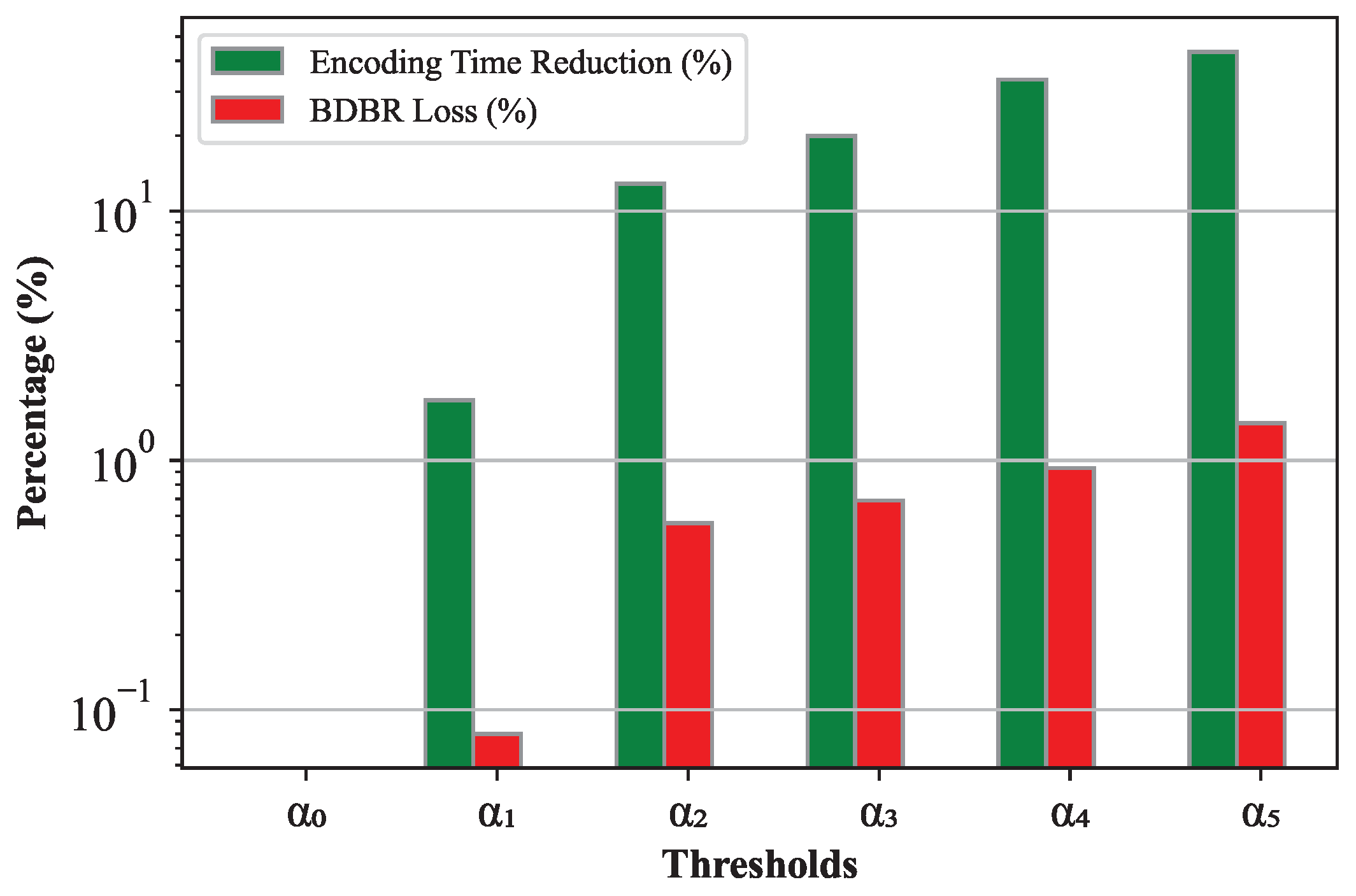
These risk intervals were evaluated using the BDBR loss as in Equation (11) and the encoding time reduction as in Equation (12). The trade-offs between time-saving and coding efficiency are illustrated in Figure 8, where it is shown clearly that trimming the risk interval and making it smaller, from to , results in a gain in terms of time-saving but at the cost of an increased BDBR loss. This explains the impact of the risk interval size on the performance of the classifiers.
These results showed that the two following risk intervals ( and ) with the predefined boundaries min and Max presented the best trade-offs in encoding efficiency and encoding time saving:
- Larger Risk Interval: = [0.30; 0.70];
- Smaller Risk Interval: = [0.45; 0.55].
Table 7 shows the different set of risk intervals values for each classifier. Indeed, the classifiers with lower accuracy have higher false positive and false negative rates, which leads to a higher uncertainty in the predictions. Therefore, a larger risk interval () is needed to account for this uncertainty. However, for classifiers with higher accuracy, smaller risk intervals () are used.
4. Experimental Results
4.1. Implementation Details and Evaluation Environment
By evaluating our proposed approach on a different set of video sequences than the video sequences used for training, it is possible to obtain a more accurate sense of how well the model will perform on new data. This is especially crucial in the context of video coding, where the characteristics of the video data can vary widely, so the model must be able to adapt to different types of video content. As a result, the test set for this study consists of the 22 CTC video sequences of JVET common test conditions [26]. These videos are then encoded using our proposed solution included in VVenC v1.3.1 [37] through its Full Feature encoder (vvencFFapp), in All Intra coding mode, over the five predefined presets, and the four QP values including 22, 27, 32 and 37.
To evaluate the results and the performance of this solution, the Bjontegaard Delta Bitrate (BDBR) [38] was adopted as a metric. It is used to measure the improvement in bitrate efficiency achieved by using a certain video coding method or technology compared to a reference method. It is defined as mentioned in [39], and it is calculated as a weighted average of the BDBR with a ratio of 6:1:1, for the luma component Y, and the two chroma components U and V of a video signal by using the following Equation (11):
The encoding time is also used to determine the time-saving noted by Encoding Time Reduction (ETR) and calculated using Equation (12),
This equation indicates that the global time saving is estimated by averaging the time differences between the needed encoding times by the original and proposed method over the four QP values (22, 27, 32 and 37). and are respectively the encoding time taken by the VVenC Reference and the VVenC Proposed encoders.
All our experiments have been performed on a cluster equipped with 48 CPUs of Intel Xeon E5-2603 v4 and a memory of 385 GB running on a Linux 5.15.0-50-generic operating system.
4.2. VVenC Encoder in All Intra Configuration Analysis: Comparison with VTM
As already stated in the previous Section 2.1, VVenC is more optimized for a Random Access (RA) use case. In fact, it includes all of VTM’s coding tools in addition to other optimizations. For instance, when compared to VTM, additional speedups are implemented for partitioning search, motion and merge search including new motion models (affine, adaptive motion vector resolution, symmetric merge vector difference, merge with motion vector difference and geometric partitioning mode), and new intra tools including intra sub-partitions and matrix-based intra prediction [23]. In addition, an optimized integer based RDOQ is included and enabled in Faster and Fast presets [23]. Consequently, VVenC has a 1.5x speedup compared to VTM, which shows clearly that VVenC in RA is closer to the VTM, while it is not optimized for the All Intra configuration use case. As mentioned in [23], the runtime difference of VVenC various presets is smaller when using the AI configuration, which is reasonable considering that the software has not been optimized for that use case. In AI configuration, each frame in a video is encoded independently without reference to any other frames, using only intra-frame prediction. This can lead to a higher quality video, but it may also require a higher bitrate and take a longer time to encode compared to coding modes that use inter-frame prediction. For these reasons, our work aims to further optimize the VVenC encoder in order to gain more in encoding time reduction while maintaining its encoding performances for AI coding significantly. Table 8 presents a side-by-side comparison of the encoding performance achieved using the two video encoders: the anchor VVenC 1.3.1 with its Slower preset, and VTM 10.0. The evaluation was conducted under the AI configuration and according to the common test conditions settings [26].
The comparison insights show that the VVenC Slower is slightly faster than the VTM 10.0 in the AI configuration, with a gain in the encoding time of 29.23%, at the cost of a degradation in BDBR by 1.10% over the six CTC classes. This is an interesting behavior, since VVenC does not include any additional coding tools optimized for this use case [23]. The slight advantage could be attributed to a different implementation of some intra-oriented coding tools [23], such as ISP and LFNST, which are implemented in VVenC inside the transform coding loop search rather than the coding unit loop search as in VTM. Therefore, this preset can be considered as the closest preset to the VTM intra encoder, which validates our choice to use it as the reference preset for evaluating our proposed approach and comparing it with the other remaining presets.
4.3. Comparison of the Slower with the Other Original Presets in AI Coding: Slow, Medium, Fast and Faster
It is important to consider the trade-offs between the encoding time and the coding efficiency when selecting a preset in the VVenC encoder. The Slower preset was utilized as the reference for evaluating the performance of the other presets, which enables a comprehensive assessment of the trade-offs between the encoding time and the encoding efficiency of each preset. Table 9 presents the comparison results in terms of Encoding Time Reduction (ETR) and BDBR Loss.
These results show that the Slow preset leads to an encoding time reduction of 54.42% with a slight increase in BDBR loss of 1.33% on average compared to Slower. This is due to the features and tools that were disabled in this preset compared to Slower. The second preset Medium provides a reduction in encoding time of 77.72% with a degradation in the video quality by around 2.49% of BDBR loss because it is optimized to achieve a good balance between encoding speed and compression efficiency, which is achieved by using a combination of compression techniques and tools, such as the reduced depth of the QT and MTT division tree [20]. The Fast and Faster presets offer a greater encoding time reduction up to 94% but at the cost of an increased BDBR loss of 9.43% and 20.41%, respectively. As the results show, going from the Slower to the Faster, a great encoding time reduction is achieved at the cost of a relative video quality degradation.
These presets are suitable for a variety of different use cases, depending on the specific needs of the user. For example, users who are more concerned with achieving the highest possible quality may choose to use one of the slower presets, while those who are more focused on speed may opt for a faster preset. By providing a range of options, the VVenC encoder allows users to find the optimal balance between performance and efficiency for their specific needs.
4.4. Performance Evaluation of the Proposed VVenC Encoder Presets: Slower, Slow, Medium, Fast and Faster
In order to evaluate our proposed approach, the 22 CTC sequences were encoded using the five presets and compared to the results of the encoding process using the Slower preset of the VVenC anchor as a reference. The experimental results shown in Table 10 demonstrate that the Slower preset resulted in an average of 30.21% in the encoding time reduction with a slight increase in BDBR loss of 0.67%. This level of BDBR loss is generally considered to be a negligible degradation in coding efficiency, indicating that this speedup in encoding time can be achieved without a significant loss in video quality.
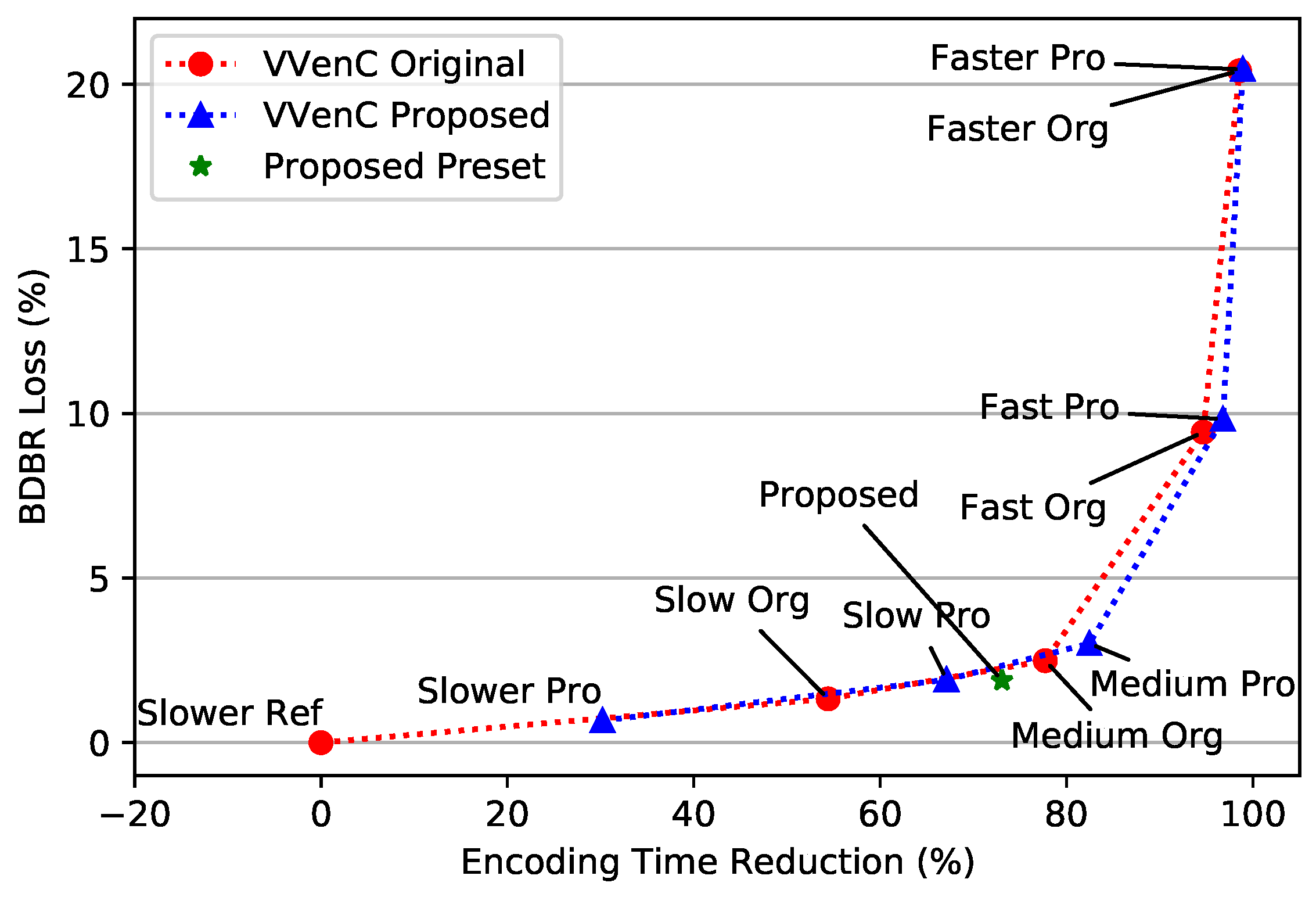
In the proposed Slower preset, the maximum ETR is presented by the FourPeople sequence by over 41.84%, and the minimum is presented by the ParkRunning3 sequence with an encoding time reduction of 10.88%. The second preset, Slow, provides a time savings of up to 67.12% and a BDBR loss of 1.91% on average compared to the reference, which is a good behavior since Slow is more optimized in terms of runtime compared to Slower. This is followed by the Medium, which resulted in about 82.46% in encoding time reduction with a loss in BDBR of 3.01%. This preset offers a balanced trade-off in encoding time and efficiency. The Fast and Faster presets accelerated the encoding process by saving time, but also caused a higher BDBR loss. For instance, the Fast preset reduced the encoding time by 96.78%, at the cost of 9.83% in BDBR loss. The Faster preset reduced the encoding time by 98.91%, but with an increased BDBR of 20.45%.
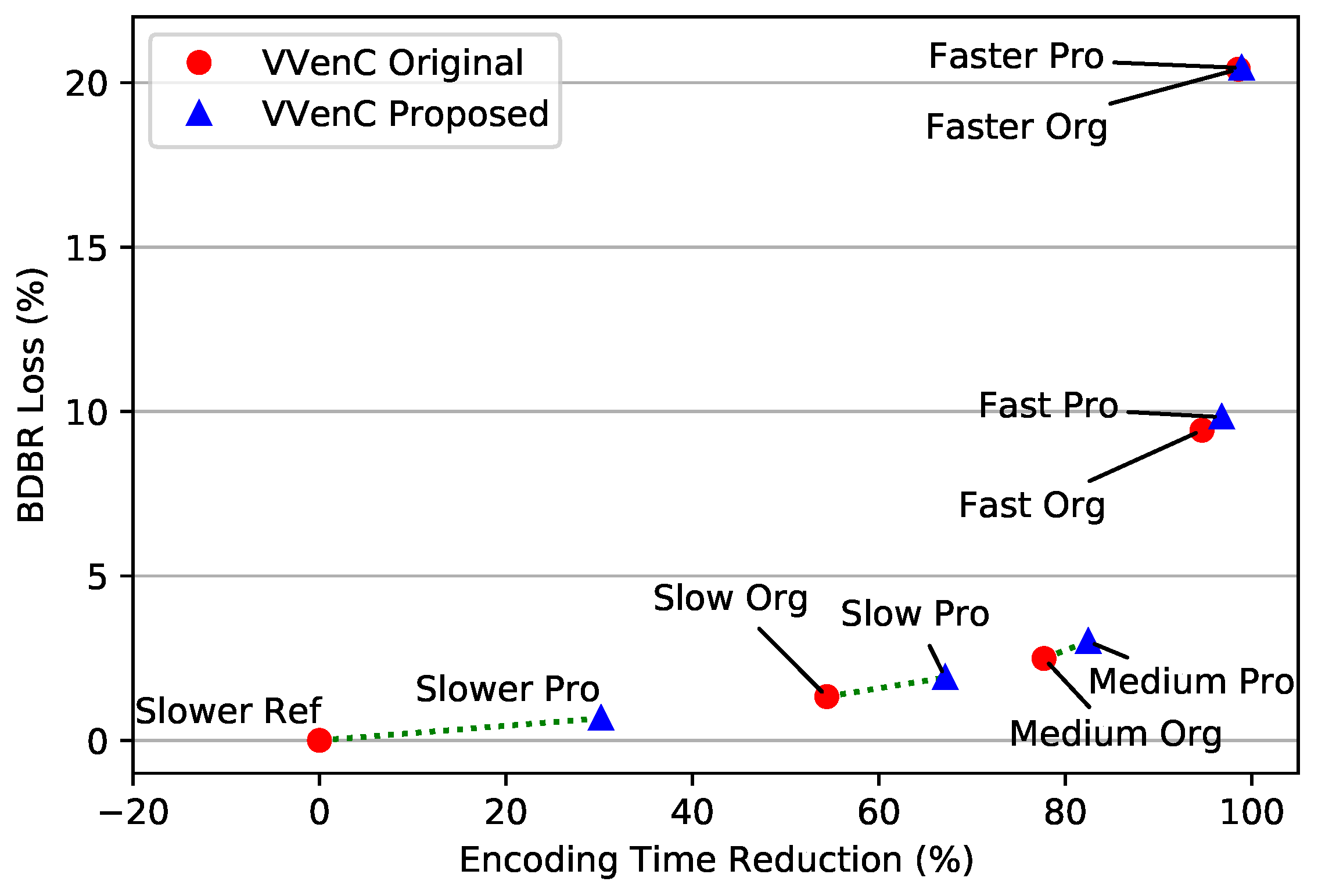
Figure 9 illustrates the trade-offs between the encoding time saving and the BDBR loss for each VVenC preset, when comparing the original and the proposed solution. It shows that the proposed approach can significantly save more time with a slight increase in BDBR degradation, which is confirmed by the results presented in Table 10.
These experimental results illustrated in Figure 9 show that we could achieve great speedups for the Slower, Slow and Medium presets. Additionally, we introduced a new preset, depicted by a green star in Figure 10, which demonstrated a significant reduction in encoding time with a reasonable increase in BDBR. This proposed preset is primarily based on the original Medium preset with some parameter adjustments.
This indicates that there is a relationship between the time-saving and the BDBR loss. In other words, as the encoding time is reduced, the quality of the encoded video will also decrease. The choice of the preset will depend on the specific needs of the user, such as the desired balance between the encoding time and video quality.
To further examine our proposed solution, we compared each preset individually using the original and the proposed encoders, and the results shown in Table 11 were achieved. Consequently, the results indicate that the proposed approach was able to significantly reduce the encoding time by over 27% on average across these presets. At the same time, the proposed approach was able to maintain a good level of image quality, as indicated by the BDBR measurements. The BDBR loss is likely to decrease slightly from the Slower preset to the Medium, which may be due to changes in the configuration files of the values of certain parameters related to the CU partitioning process, such as the maximum depth of the QTMTT structure and the maximum CTU size.
Overall, these results demonstrate that the proposed approach was able to effectively balance the trade-off between encoding time and image quality. This is an important consideration for many users, as the encoding process can be resource-intensive and time-consuming. By using the proposed approach, users may be able to save time and resources while still maintaining a high level of image quality.
4.5. Comparison with the State-of-the-Art Techniques
In this subsection, a comparison of the proposed solution with other state-of-the-art approaches was conducted in terms of encoding time reduction (ETR) and BDBR loss. Table 12 shows the average trade-offs over the different video sequences’ classes. The state-of-the-art approaches were embedded and evaluated using the VTM reference software, while the proposed approach was integrated into the VVenC 1.3.1 [37] using the Slower preset as a reference. In addition, a new preset was proposed to further increase the speed of the encoding process with a slight BDBR degradation. These two presets show a great improvement in the encoding process by saving time while maintaining a significant image quality. It is important to note that a direct comparison of the proposed approach implemented in the VVenC encoder with the state-of-the-art works that utilize the VTM reference software may not be entirely significant. Therefore, a more appropriate comparison would be to compare the proposed approach with other state-of-the-art works embedded on the VVenC encoder and that have been optimized for similar use cases.
The results in Table 12 showed that, in terms of encoding efficiency, the best results measured by the BDBR metric were achieved by our proposed approach using the Slower preset followed by the approach presented by Saldanha in [13] and Zhang in [31] with values of 1.42% and 1.52%, respectively, while Guoqing in [33] achieved reached a higher degradation in BDBR of 2.71%. In terms of ETR, our proposed preset outperforms the other cited works with an average of 73.07%, followed by the solutions of Guoqing [33], Zhang [31], Saldanha [13], and finally our proposed solution with the Slower preset.
Indeed, the Slower preset offers the lowest BDBR degradation by only 0.67% with a significant time savings of 31.21%, which is a good trade-off in comparison with the other mentioned works. Concerning the proposed preset, it leads to a larger ability to save time by up to 73.07% over these state-of-the-art works with a reasonable increase in BDBR loss of 1.89%. Overall, the proposed solution demonstrated good performance in comparison to the other works by achieving a good balance between BDBR degradation and encoding time reduction. As also shown in Figure 10, the proposed preset represented by the green star is under the two curves of the original and proposed VVenC presets. This confirms clearly that it is able to save more time at the cost of a reasonable BDBR loss of 1.89% compared to the all remaining presets. These results indicate that the proposed solution is a promising approach, although there is potential for further improvements in the encoding process efficiency.
5. Conclusions
In this paper, we presented a new approach based on LightGBM models to accelerate the CU partitioning process in the VVC intra coding. This approach integrated into the VVenC encoder extracts CU features and uses them to feed the LightGBM classifiers, which can directly predict the most probable split mode among all the available options in the QTMTT structure. Additionally, predefined risk intervals were used for each classifier to further improve their classification performance. We also proposed a new preset that offers a good balance between quality and speed, by saving around 73.07% in the encoding time with only 1.89% in BDBR loss compared to the other presets. The experiments showed that our approach can significantly reduce encoding time while maintaining a good encoding efficiency compared to other state-of-the-art techniques. Overall, the proposed approach can save time and resources while providing a significant encoding efficiency, which makes it a potentially attractive choice for a wide range of applications.
Author Contributions
Conceptualization, I.T., D.M., A.M. and A.A.; methodology, I.T., D.M., A.M. and A.A.; software, I.T.; validation D.M., A.M. and A.A.; formal analysis, I.T., D.M., A.M. and A.A.; investigation, I.T., D.M., A.M. and A.A.; data curation, I.T.; writing—original draft preparation, I.T.; writing—review and editing, D.M., A.M. and A.A.; visualization, I.T., D.M., A.M. and A.A.; supervision, D.M., A.M. and A.A. All authors have read and agreed to the published version of the manuscript.
Funding
This work was financially supported by Campus France and the Moroccan National Center of Scientific and Technology Research (CNRST) through the PHC Maghreb project Eco-VVC (Grant No. 45988WG).
Data Availability Statement
The data that support the findings of this study are available from the corresponding author, Ibrahim Taabane, upon reasonable request.
Acknowledgments
We would like to thank Campus France and the Moroccan CNRST for their financial support within the framework of the PHC Maghreb project number 23MAGH21 (45988WG). We also thank INSA Rennes and USMBA University for their support and access to their resources.
Conflicts of Interest
All the authors declare that they have no conflict of interest.
References
- Cisco Annual Internet Report—Cisco Annual Internet Report (2018–2023) White Paper. 2022. Available online: https://www.cisco.com/c/en/us/solutions/collateral/executive-perspectives/annual-internet-report/white-paper-c11-741490.html (accessed on 1 July 2022).
- Sullivan, G.J.; Ohm, J.R.; Han, W.J.; Wiegand, T. Overview of the high efficiency video coding (HEVC) standard. IEEE Trans. Circuits Syst. Video Technol. 2012, 22, 1649–1668. [Google Scholar] [CrossRef]
- Bross, B.; Wang, Y.K.; Ye, Y.; Liu, S.; Chen, J.; Sullivan, G.J.; Ohm, J.R. Overview of the Versatile Video Coding (VVC) Standard and its Applications. IEEE Trans. Circuits Syst. Video Technol. 2021, 31, 3736–3764. [Google Scholar] [CrossRef]
- Kammoun, A.; Hamidouche, W.; Philippe, P.; Déforges, O.; Belghith, F.; Masmoudi, N.; Nezan, J.F. Forward-inverse 2D hardware implementation of approximate transform core for the VVC standard. IEEE Trans. Circuits Syst. Video Technol. 2019, 30, 4340–4354. [Google Scholar] [CrossRef]
- Farhat, I.; Hamidouche, W.; Grill, A.; Menard, D.; Déforges, O. Lightweight hardware implementation of VVC transform block for ASIC decoder. In Proceedings of the ICASSP 2020—2020 IEEE International Conference on Acoustics, Speech and Signal Processing (ICASSP), Barcelona, Spain, 4–8 May 2020; pp. 1663–1667. [Google Scholar] [CrossRef] [Green Version]
- Yibo, F.; Jiro, K.; Heming, S.; Xiaoyang, Z.; Yixuan, Z. A minimal adder-oriented 1D DST-VII/DCT-VIII hardware implementation for VVC standard. In Proceedings of the 2019 32nd IEEE International System-on-Chip Conference (SOCC), Singapore, 3–6 September 2019; pp. 176–180. [Google Scholar] [CrossRef]
- Gao, H.; Chen, X.; Esenlik, S.; Chen, J.; Steinbach, E. Decoder-side motion vector refinement in VVC: Algorithm and hardware implementation considerations. IEEE Trans. Circuits Syst. Video Technol. 2020, 31, 3197–3211. [Google Scholar] [CrossRef]
- Lei, M.; Luo, F.; Zhang, X.; Wang, S.; Ma, S. Look-ahead prediction based coding unit size pruning for VVC intra coding. In Proceedings of the 2019 IEEE International Conference on Image Processing (ICIP), Taipei, Taiwan, 22–25 September 2019; pp. 4120–4124. [Google Scholar] [CrossRef]
- Cui, J.; Zhang, T.; Gu, C.; Zhang, X.; Ma, S. Gradient-based early termination of CU partition in VVC intra coding. In Proceedings of the 2020 Data Compression Conference (DCC), Snowbird, UT, USA, 24–27 March 2020; pp. 103–112. [Google Scholar] [CrossRef]
- Fan, Y.; Sun, H.; Katto, J.; Ming’E, J. A fast QTMT partition decision strategy for VVC intra prediction. IEEE Access 2020, 8, 107900–107911. [Google Scholar] [CrossRef]
- Tissier, A.; Hamidouche, W.; Mdalsi, S.B.D.; Vanne, J.; Galpin, F.; Menard, D. Machine Learning based Efficient QT-MTT Partitioning Scheme for VVC Intra Encoders. IEEE Trans. Circuits Syst. Video Technol. 2023. [Google Scholar] [CrossRef]
- Li, T.; Xu, M.; Tang, R.; Chen, Y.; Xing, Q. DeepQTMT: A Deep Learning Approach for Fast QTMT-Based CU Partition of Intra-Mode VVC. IEEE Trans. Image Process. 2021, 30, 5377–5390. [Google Scholar] [CrossRef] [PubMed]
- Saldanha, M.; Sanchez, G.; Marcon, C.; Agostini, L. Configurable Fast Block Partitioning for VVC Intra Coding Using Light Gradient Boosting Machine. IEEE Trans. Circuits Syst. Video Technol. 2022, 32, 3947–3960. [Google Scholar] [CrossRef]
- Chen, F.; Ren, Y.; Peng, Z.; Jiang, G.; Cui, X. A fast CU size decision algorithm for VVC intra prediction based on support vector machine. Multimed. Tools Appl. 2020, 79, 27923–27939. [Google Scholar] [CrossRef]
- He, Q.; Wu, W.; Luo, L.; Zhu, C.; Guo, H. Random Forest Based Fast CU Partition for VVC Intra Coding. In Proceedings of the IEEE International Symposium on Broadband Multimedia Systems and Broadcasting (BMSB), Chengdu, China, 4–6 August 2021; pp. 31–34. [Google Scholar] [CrossRef]
- Vo, T.H.; Nguyen, N.T.K.; Kha, Q.H.; Le, N.Q.K. On the road to explainable AI in drug-drug interactions prediction: A systematic review. Comput. Struct. Biotechnol. J. 2022, 20, 2112–2123. [Google Scholar] [CrossRef] [PubMed]
- Lam, L.H.T.; Do, D.T.; Diep, D.T.N.; Nguyet, D.L.N.; Truong, Q.D.; Tri, T.T.; Thanh, H.N.; Le, N.Q.K. Molecular subtype classification of low-grade gliomas using magnetic resonance imaging-based radiomics and machine learning. NMR Biomed. 2022, 35, e4792. [Google Scholar] [CrossRef] [PubMed]
- El Ydrissi, M.; Ghennioui, H.; Ghali Bennouna, E.; Alae, A.; Abraim, M.; Taabane, I.; Farid, A. Dust InSMS: Intelligent soiling measurement system for dust detection on solar mirrors using computer vision methods. Expert Syst. Appl. 2023, 211, 118646. [Google Scholar] [CrossRef]
- Random Forest vs. Lightgbm. Available online: https://mljar.com/machine-learning/lightgbm-vs-random-forest/ (accessed on 30 July 2022).
- Wieckowski, A.; Brandenburg, J.; Hinz, T.; Bartnik, C.; George, V.; Hege, G.; Helmrich, C.; Henkel, A.; Lehmann, C.; Stoffers, C.; et al. VVenC: An Open in addition, Optimized VVC Encoder Implementation. In Proceedings of the IEEE International Conference on Multimedia Expo Workshops (ICMEW), Shenzhen, China, 5–9 July 2021; pp. 1–2. [Google Scholar] [CrossRef]
- Ke, G.; Meng, Q.; Finley, T.; Wang, T.; Chen, W.; Ma, W.; Ye, Q.; Liu, T.Y. LightGBM: A Highly Efficient Gradient Boosting Decision Tree. In Proceedings of the Advances in Neural Information Processing Systems; Curran Associates, Inc.: Long Beach, CA, USA, 2017; Volume 30, Available online: https://proceedings.neurips.cc/paper/2017/file/6449f44a102fde848669bdd9eb6b76fa-Paper.pdf (accessed on 1 July 2022).
- VTM VVC Reference Software. Available online: https://vcgit.hhi.fraunhofer.de/jvet/VVCSoftware_VTM (accessed on 1 July 2022).
- Wieckowski, A.; Stoffers, C.; Bross, B.; Marpe, D. VVenC: An open optimized VVC encoder in versatile application scenarios. In Proceedings of the Applications of Digital Image Processing XLIV; Tescher, A.G., Ebrahimi, T., Eds.; International Society for Optics and Photonics; SPIE: San Diego, CA, USA, 2021; Volume 11842, p. 118420H. [Google Scholar] [CrossRef]
- Brandenburg, J.; Wieckowski, A.; Henkel, A.; Bross, B.; Marpe, D. Pareto-optimized coding configurations for VVenC, a fast and efficient VVC encoder. In Proceedings of the IEEE 23rd International Workshop on Multimedia Signal Processing (MMSP 2021), Tampere, Finland, 6–8 October 2021. [Google Scholar] [CrossRef]
- Sullivan, G.; Wiegand, T. Rate-distortion optimization for video compression. IEEE Signal Process. Mag. 1998, 15, 74–90. [Google Scholar] [CrossRef] [Green Version]
- Bossen, F.; Boyce, J.; Suehring, X.; Li, X.; Seregin, V. JVET Common Test Conditions and Software Reference Configurations for SDR Video 2019. In Proceedings of the JVET 14th Meeting, Geneva, Switzerland, 19–27 March 2019. [Google Scholar]
- Tissier, A.; Mercat, A.; Amestoy, T.; Hamidouche, W.; Vanne, J.; Menard, D. Complexity Reduction Opportunities in the Future VVC Intra Encoder. In Proceedings of the IEEE 21st International Workshop on Multimedia Signal Processing (MMSP 2019), Kuala Lumpur, Malaysia, 27–29 September 2019. [Google Scholar] [CrossRef] [Green Version]
- Fu, T.; Zhang, H.; Mu, F.; Chen, H. Fast CU partitioning algorithm for H.266/VVC intra-frame coding. In Proceedings of the IEEE International Conference on Multimedia and Expo, Shanghai, China, 8–12 July 2019; pp. 55–60. [Google Scholar] [CrossRef]
- Zhang, Q.; Guo, R.; Jiang, B.; Su, R. Fast CU Decision-Making Algorithm Based on DenseNet Network for VVC. IEEE Access 2021, 9, 119289–119297. [Google Scholar] [CrossRef]
- Hoangvan, X.; Nguyenquang, S.; Dinhbao, M.; Dongoc, M.; Duong, D.T. Fast QTMT for H.266/VVC Intra Prediction using Early-Terminated Hierarchical CNN model. In Proceedings of the 2021 International Conference on Advanced Technologies for Communications (ATC), Ho Chi Minh City, Vietnam, 14–16 October 2021; pp. 195–200. [Google Scholar] [CrossRef]
- Zhang, S.; Feng, S.; Chen, J.; Zhou, C.; Yang, F. A GCN-based fast CU partition method of intra-mode VVC. J. Vis. Commun. Image Represent. 2022, 88, 103621. [Google Scholar] [CrossRef]
- Liu, Y.; Wang, Y.; Zhang, J. New Machine Learning Algorithm: Random Forest. In Proceedings of the Information Computing and Applications; Liu, B., Ma, M., Chang, J., Eds.; Springer: Berlin/Heidelberg, Germany, 2012; pp. 246–252. [Google Scholar] [CrossRef]
- Wu, G.; Huang, Y.; Zhu, C.; Song, L.; Zhang, W. SVM based fast CU partitioning algorithm for VVC intra coding. In Proceedings of the IEEE International Symposium on Circuits and Systems, Daegu, Republic of Korea, 22–28 May 2021. [Google Scholar] [CrossRef]
- Akiba, T.; Sano, S.; Yanase, T.; Ohta, T.; Koyama, M. Optuna: A Next-generation Hyperparameter Optimization Framework. In Proceedings of the 25rd ACM SIGKDD International Conference on Knowledge Discovery and Data Mining, Anchorage, AK, USA, 4–8 August 2019. [Google Scholar] [CrossRef]
- Taabane, I.; Menard, D.; Mansouri, A.; Ahaitouf, A. A Fast CU Partition Algorithm for VVenC Encoder in Intra Configuration. In Proceedings of the 2022 IEEE Workshop on Signal Processing Systems (SiPS), Rennes, France, 2–4 November 2022; pp. 1–6. [Google Scholar] [CrossRef]
- Bergstra, J.; Bardenet, R.; Bengio, Y.; Kégl, B. Algorithms for hyper-parameter optimization. In Proceedings of the 24th International Conference on Neural Information Processing Systems, Granada, Spain, 12–15 December 2011; pp. 2546–2554. [Google Scholar]
- Fraunhofer Versatile Video Encoder (VVENC). Available online: https://github.com/fraunhoferhhi/vvenc/releases/tag/v1.3.1 (accessed on 23 February 2023).
- Bjontegaard, G. Calculation of Average PSNR Differences between RD-Curves. VCEG-M33 2001. Available online: https://cir.nii.ac.jp/crid/1571980074917801984 (accessed on 28 January 2023).
- Ström, J.; Andersson, K.; Sjöberg, R.; Segall, A.; Bossen, F.; Sullivan, G.; Ohm, J.; Tourapis, A. Working practices using objective metrics for evaluation of video coding efficiency experiments. ITU-T ISO/IEC JTC 2021, 1, 23002-8. Available online: https://www.itu.int/pub/T-TUT-ASC-2020-HSTP1 (accessed on 23 February 2023).
Figure 1.
The main steps of a VVC encoder.

Figure 2.
QTMTT structure for the partitioning block in VVC. (a) Available CU split modes in VVC. (b) Example of a QTMTT scheme division for a CTU.
Figure 2.
QTMTT structure for the partitioning block in VVC. (a) Available CU split modes in VVC. (b) Example of a QTMTT scheme division for a CTU.

Figure 3.
Illustration of the QTMTT scheme partitioning on an encoded video sequence.

Figure 4.
Framework of the proposed approach for CU partitioning decision using LightGBM models integrated into the VVenC encoder.
Figure 4.
Framework of the proposed approach for CU partitioning decision using LightGBM models integrated into the VVenC encoder.

Figure 5.
The proposed approach algorithm and its implementation flowchart. (a) The proposed algorithm for CU partition selection. (b) Flowchart of the proposed approach.
Figure 5.
The proposed approach algorithm and its implementation flowchart. (a) The proposed algorithm for CU partition selection. (b) Flowchart of the proposed approach.

Figure 6.
CU block for feature extraction. (a) Squared Sub-CUs blocks. (b) Rectangular Sub-CUs blocks.
Figure 6.
CU block for feature extraction. (a) Squared Sub-CUs blocks. (b) Rectangular Sub-CUs blocks.

Figure 7.
Risk interval in machine learning.

Figure 8.
Risk intervals’ trade-offs in terms of encoding time reduction and BDBR loss for a video sequence encoded using different thresholds for classification.
Figure 8.
Risk intervals’ trade-offs in terms of encoding time reduction and BDBR loss for a video sequence encoded using different thresholds for classification.

Figure 9.
Original vs. proposed VVenC encoder presets’ speedups.

Figure 10.
Original vs. proposed VVenC encoder presets’ trade-offs in terms of ETR (%) and BDBR (%).
Figure 10.
Original vs. proposed VVenC encoder presets’ trade-offs in terms of ETR (%) and BDBR (%).


Table 1.
Possible split modes according to the CU size.
| Width | 64 | 32 | 16 | 8 | 4 | |
|---|---|---|---|---|---|---|
| Height | ||||||
| 64 | QT | - | ||||
| 32 | - | All | BT, TT | BT TTH | BTH TTH | |
| 16 | BT, TT | All | ||||
| 8 | BT, TTV | BT | BTH | |||
| 4 | BTV, TTV | BTV | - | |||
Table 2.
Comparison of the state-of-the-art works.
| Approach | Reference Software | Technique | BDBR Loss (%) | Complexity Reduction (%) |
|---|---|---|---|---|
| Jing Cui [9] | VTM 5.0 | Heuristic | 1.23 | 51.01 |
| Fu [28] | VTM 1.0 | Heuristic | 1.02 | 45.00 |
| Tissier [11] | VTM 10.2 | ML+DL | 0.79 | 47.4 |
| Saldanha [13] | VTM 10.0 | ML (LightGBM) | 1.42 | 54.20 |
| Chen [14] | VTM 4.0 | ML (SVM) | 1.62 | 51.23 |
| Quan [15] | VTM 7.0 | ML (RF) | 1.21 | 57.00 |
| Guoqing [33] | VTM 10.0 | ML (SVM) | 2.71 | 63.16 |
| Li [12] | VTM 7.0 | DL | 1.32 | 44.65 |
| Qiuwen [29] | VTM 10.0 | DL | 1.80 | 53.98 |
| Hoang [30] | VTM 12.1 | DL | 1.39 | 30.29 |
| Zhang [31] | VTM 10.0 | DL | 1.52 | 61.15 |
Table 3.
Distribution of our dataset by image resolutions.
| Resolution | 240p | 480p | 720p | 1080p | 4K | 8K | Total |
|---|---|---|---|---|---|---|---|
| Number of images | 500 | 500 | 579 | 2557 | 654 | 418 | 5208 |
Table 4.
Split modes and their corresponding number of sub-CUs parts.
| Split Mode (j) | QT | BTH | BTV | TTH | TTV |
|---|---|---|---|---|---|
| Number of sub-CUs parts (k) | 4 | 2 | 2 | 3 | 3 |
Table 5.
Training parameters for our LightGBM models.
| Parameter Name | Parameter Setting |
|---|---|
| Number of features | 65 |
| Number of estimators | 30 |
| Maximum Depth | 15 |
| Learning rate | 0.05 |
| Boosting type | GBDT |
Table 6.
Accuracy and F1-score for each classifier.
| Classifier | Metric | 32 × 32 | 32 × 16 | 32 × 8 | 8 × 32 | 16 × 32 | 16 × 16 | 16 × 8 | 8 × 16 |
|---|---|---|---|---|---|---|---|---|---|
| S-NS | Accuracy (%) | 98.28 | 96.21 | 94.27 | 95.77 | 96.36 | 97.46 | 93.51 | 92.83 |
| F1 score (%) | 97.29 | 96.12 | 93.95 | 94.85 | 96.14 | 97.22 | 93.18 | 92.41 | |
| QT-MTT | Accuracy (%) | 86.65 | - | - | - | - | 82.24 | - | - |
| F1 score (%) | 86.73 | - | - | - | - | 82.17 | - | - | |
| Hor-Ver | Accuracy (%) | 87.60 | 90.21 | 84.17 | 83.23 | 93.16 | 87.35 | 77.51 | 79.83 |
| F1 score (%) | 87.52 | 89.95 | 84.27 | 83.38 | 92.88 | 87.21 | 77.35 | 78.16 | |
| BH-TH | Accuracy (%) | 84.55 | 87.21 | - | 85.64 | 93.16 | 87.76 | - | 74.36 |
| F1 score (%) | 84.13 | 87.38 | - | 85.14 | 92.96 | 86.94 | - | 74.12 | |
| BV-TV | Accuracy (%) | 85.18 | 85.67 | 81.62 | - | 72.73 | 82.68 | 79.56 | - |
| F1 score (%) | 85.34 | 84.03 | 81.11 | - | 70.98 | 81.87 | 77.12 | - |
Table 7.
Risk intervals for each classifier.
| Classifier | 32 × 32 | 32 × 16 | 32 × 8 | 8 × 32 | 16 × 32 | 16 × 16 | 16 × 8 | 8 × 16 |
|---|---|---|---|---|---|---|---|---|
| S-NS | ||||||||
| QT-MTT | - | - | - | - | - | - | ||
| Hor-Ver | ||||||||
| BH-TH | - | - | ||||||
| BV-TV | - | - |
Table 8.
VVenC encoder in All Intra configuration analysis compared to the VTM 10.0 encoder.
| Presets | Slower | |
|---|---|---|
| Class | BDBR (%) | ΔETR (%) |
| A1 (3840 × 2160) | 1.14 | 32.37 |
| A2 (3840 × 2160) | 3.85 | 36.28 |
| B (1920 × 1080) | 0.28 | 29.57 |
| C (832 × 480) | 0.72 | 25.25 |
| D (416 × 240) | 0.73 | 24.07 |
| E (1280 × 720) | −0.12 | 27.88 |
| Average | 1.10 | 29.23 |
Table 9.
Trade-offs between Encoding Time Reduction ETR (%) and coding efficiency BDBR (%): results of the VVenC original presets compared to the Slower original.
Table 9.
Trade-offs between Encoding Time Reduction ETR (%) and coding efficiency BDBR (%): results of the VVenC original presets compared to the Slower original.
| Presets | Slow | Medium | Fast | Faster | ||||
|---|---|---|---|---|---|---|---|---|
| Class | BDBR (%) | ΔETR (%) | BDBR (%) | ΔETR (%) | BDBR (%) | ΔETR (%) | BDBR (%) | ΔETR (%) |
| A1 | 1.21 | 54.78 | 1.61 | 73.73 | 8.05 | 92.19 | 18.02 | 97.83 |
| A2 | 1.48 | 51.34 | 2.46 | 74.87 | 10.83 | 94.07 | 21.38 | 98.58 |
| B | 1.40 | 54.85 | 2.50 | 78.11 | 9.32 | 94.90 | 20.46 | 98.70 |
| C | 1.49 | 55.31 | 3.00 | 80.55 | 9.60 | 95.95 | 21.24 | 98.99 |
| D | 1.02 | 57.11 | 2.34 | 81.50 | 8.26 | 96.17 | 17.38 | 99.10 |
| E | 1.39 | 53.14 | 3.00 | 77.56 | 10.52 | 94.76 | 23.99 | 98.17 |
| Average | 1.33 | 54.42 | 2.49 | 77.72 | 9.43 | 94.67 | 20.41 | 98.56 |
Table 10.
Trade-offs between Encoding Time Reduction ETR (%) and encoding efficiency BDBR (%): results of the proposed solution of the five presets compared to the Slower original.
Table 10.
Trade-offs between Encoding Time Reduction ETR (%) and encoding efficiency BDBR (%): results of the proposed solution of the five presets compared to the Slower original.
| Presets | Slower | Slow | Medium | Fast | Faster | ||||||
|---|---|---|---|---|---|---|---|---|---|---|---|
| Class | Video | BDBR (%) | ΔETR (%) | BDBR (%) | ΔETR (%) | BDBR (%) | ΔETR (%) | BDBR (%) | ΔETR (%) | BDBR (%) | ΔETR (%) |
| A1 | Campfire | 0.49 | 32.56 | 1.71 | 79.94 | 2.56 | 81.15 | 9.88 | 95.68 | 16.06 | 98.37 |
| Tango2 | -0.40 | 30.76 | 0.76 | 77.61 | 1.07 | 68.94 | 8.30 | 96.15 | 21.56 | 97.58 | |
| FoodMarket4 | 0.23 | 32.15 | 1.66 | 69.96 | 1.86 | 69.40 | 6.51 | 94.89 | 16.55 | 97.89 | |
| Average | 0.11 | 31.82 | 1.38 | 75.84 | 1.83 | 73.16 | 8.23 | 95.57 | 18.06 | 97.95 | |
| A2 | DaylightRoad2 | 0.94 | 20.61 | 2.33 | 67.90 | 3.57 | 79.57 | 14.74 | 96.88 | 26.69 | 98.95 |
| CatRobot1 | 0.50 | 18.21 | 2.28 | 62.54 | 3.31 | 75.36 | 11.36 | 95.51 | 24.05 | 98.45 | |
| ParkRunning3 | 0.61 | 10.88 | 1.72 | 56.81 | 2.17 | 74.53 | 8.10 | 94.75 | 13.49 | 98.48 | |
| Average | 0.68 | 16.57 | 2.11 | 62.42 | 3.02 | 76.49 | 11.40 | 95.71 | 21.41 | 98.63 | |
| B | MarketPlace | 0.45 | 34.31 | 1.63 | 64.70 | 2.08 | 85.77 | 7.35 | 98.97 | 14.90 | 99.52 |
| RitualDance | 0.94 | 38.07 | 2.19 | 65.75 | 3.11 | 87.83 | 8.62 | 98.88 | 17.59 | 99.28 | |
| BQTerrace | 1.32 | 33.92 | 2.95 | 68.56 | 4.36 | 89.39 | 11.04 | 98.44 | 22.63 | 99.42 | |
| BasketBallDrive | 0.49 | 33.25 | 1.99 | 67.92 | 3.39 | 87.74 | 12.08 | 99.62 | 27.52 | 99.58 | |
| Cactus | 0.73 | 30.62 | 1.77 | 66.43 | 2.93 | 88.22 | 9.90 | 98.79 | 19.85 | 99.50 | |
| Average | 0.79 | 34.03 | 2.11 | 66.67 | 3.17 | 87.79 | 9.80 | 98.94 | 20.50 | 99.46 | |
| C | PartyScene | 0.41 | 33.88 | 1.38 | 68.25 | 2.53 | 89.60 | 8.05 | 97.29 | 15.41 | 99.56 |
| BQMall | 0.91 | 27.94 | 2.20 | 66.40 | 3.75 | 88.56 | 11.51 | 97.70 | 22.95 | 99.70 | |
| BasketBallDrill | 1.36 | 23.20 | 3.65 | 63.24 | 5.63 | 87.39 | 12.00 | 98.28 | 30.61 | 99.61 | |
| RaceHorsesC | 0.51 | 26.56 | 1.30 | 65.91 | 2.41 | 88.55 | 7.96 | 97.76 | 15.83 | 99.56 | |
| Average | 0.80 | 27.90 | 2.13 | 65.95 | 3.58 | 88.53 | 9.88 | 97.76 | 21.20 | 99.61 | |
| D | BQSquare | 0.37 | 30.30 | 1.45 | 67.37 | 2.69 | 88.98 | 8.80 | 97.88 | 16.02 | 99.59 |
| BlowingBubbles | 0.47 | 37.37 | 1.11 | 68.34 | 2.26 | 87.85 | 7.29 | 96.96 | 15.66 | 99.51 | |
| BasketBallPass | 0.76 | 26.63 | 1.78 | 67.20 | 3.30 | 86.99 | 10.08 | 97.46 | 20.76 | 99.44 | |
| RaceHorsesD | 0.48 | 32.85 | 1.15 | 67.83 | 2.32 | 87.23 | 7.85 | 97.18 | 17.01 | 99.44 | |
| Average | 0.52 | 31.79 | 1.37 | 67.69 | 2.64 | 87.76 | 8.51 | 97.37 | 17.36 | 99.50 | |
| E | FourPeople | 1.32 | 41.84 | 2.58 | 64.86 | 3.99 | 81.87 | 10.93 | 95.67 | 22.96 | 98.68 |
| Johnny | 1.11 | 39.34 | 2.41 | 66.22 | 4.05 | 81.14 | 11.71 | 95.21 | 25.40 | 98.14 | |
| KristenAndSara | 0.95 | 36.29 | 2.17 | 61.48 | 3.50 | 80.10 | 10.82 | 95.05 | 24.21 | 98.21 | |
| Average | 1.13 | 39.16 | 2.39 | 64.19 | 3.85 | 81.04 | 11.15 | 95.31 | 24.19 | 98.34 | |
| Classes average | 0.67 | 30.21 | 1.91 | 67.12 | 3.01 | 82.46 | 9.83 | 96.78 | 20.45 | 98.91 | |
Table 11.
Comparison of each preset individually using the original and the proposed encoders.
| Preset | Encoding Time Reduction (%) | BDBR Loss (%) |
|---|---|---|
| Slower | 30.21 | 0.67 |
| Slow | 28.12 | 0.58 |
| Medium | 23.67 | 0.52 |
| Fast | 21.98 | 0.38 |
| Faster | 25.63 | 0.05 |
Table 12.
Performance comparison of the proposed solution with the state-of-the-art approaches in AI coding.
Table 12.
Performance comparison of the proposed solution with the state-of-the-art approaches in AI coding.
| Approach | Saldanha [13] | Guoqing [33] | Zhang [31] | Slower Proposed | Proposed Preset | |||||
|---|---|---|---|---|---|---|---|---|---|---|
| Class | BDBR (%) | ΔETR (%) | BDBR (%) | ΔETR (%) | BDBR (%) | ΔETR (%) | BDBR (%) | ΔETR (%) | BDBR (%) | ΔETR (%) |
| A1 | 1.05 | 53.39 | 2.18 | 58.70 | 1.65 | 61.19 | 0.11 | 31.82 | 1.25 | 74.75 |
| A2 | 1.11 | 52.63 | 2.25 | 63.11 | 1.87 | 63.04 | 0.68 | 16.57 | 2.01 | 74.31 |
| B | 1.40 | 58.26 | 2.87 | 66.93 | 1.52 | 64.43 | 0.79 | 34.03 | 2.04 | 77.89 |
| C | 1.65 | 51.99 | 2.92 | 62.27 | 1.39 | 58.61 | 0.80 | 27.90 | 2.17 | 72.15 |
| D | 1.24 | 49.92 | 1.98 | 60.01 | 0.95 | 56.35 | 0.52 | 31.79 | 1.47 | 69.87 |
| E | 2.07 | 58.44 | 4.08 | 66.78 | 1.97 | 62.74 | 1.13 | 39.16 | 2.38 | 69.48 |
| Average | 1.42 | 54.20 | 2.71 | 63.16 | 1.52 | 61.15 | 0.67 | 30.21 | 1.89 | 73.07 |
Disclaimer/Publisher’s Note: The statements, opinions and data contained in all publications are solely those of the individual author(s) and contributor(s) and not of MDPI and/or the editor(s). MDPI and/or the editor(s) disclaim responsibility for any injury to people or property resulting from any ideas, methods, instructions or products referred to in the content. |
© 2023 by the authors. Licensee MDPI, Basel, Switzerland. This article is an open access article distributed under the terms and conditions of the Creative Commons Attribution (CC BY) license (https://creativecommons.org/licenses/by/4.0/).
Share and Cite
MDPI and ACS Style
Taabane, I.; Menard, D.; Mansouri, A.; Ahaitouf, A. Machine Learning Based Fast QTMTT Partitioning Strategy for VVenC Encoder in Intra Coding. Electronics 2023, 12, 1338. https://doi.org/10.3390/electronics12061338
AMA Style
Taabane I, Menard D, Mansouri A, Ahaitouf A. Machine Learning Based Fast QTMTT Partitioning Strategy for VVenC Encoder in Intra Coding. Electronics. 2023; 12(6):1338. https://doi.org/10.3390/electronics12061338
Chicago/Turabian StyleTaabane, Ibrahim, Daniel Menard, Anass Mansouri, and Ali Ahaitouf. 2023. "Machine Learning Based Fast QTMTT Partitioning Strategy for VVenC Encoder in Intra Coding" Electronics 12, no. 6: 1338. https://doi.org/10.3390/electronics12061338
Note that from the first issue of 2016, this journal uses article numbers instead of page numbers. See further details here.