
Timeslot Scheduling with Reinforcement Learning Using a Double Deep Q-Network

1
Department of AI & Informatics, Sangmyung University, Seoul 03016, Republic of Korea
2
Electronics and Telecommunications Research Institute (ETRI), Daejeon 34129, Republic of Korea
3
Network Engineering Major, University of Science and Technology, Daejeon 34113, Republic of Korea
4
Department of Human-Centered Artificial Intelligence, Sangmyung University, Seoul 03016, Republic of Korea
*
Author to whom correspondence should be addressed.
Electronics 2023, 12(4), 1042; https://doi.org/10.3390/electronics12041042
Submission received: 18 January 2023
/
Revised: 11 February 2023
/
Accepted: 16 February 2023
/
Published: 20 February 2023
(This article belongs to the Section Networks)
Abstract
:Adopting reinforcement learning in the network scheduling area is getting more attention than ever because of its flexibility in adapting to the dynamic changes of network traffic and network status. In this study, a timeslot scheduling algorithm for traffic, with similar requirements but different priorities, is designed using a double deep q-network (DDQN), a reinforcement learning algorithm. To evaluate the behavior of the DDQN agent, a reward function is defined based on the difference between the estimated delay and the deadline of packets transmitted at the timeslot, and on the priority of packets. The simulation showed that the designed scheduling algorithm performs better than existing algorithms, such as the strict priority (SP) or weighted round robin (WRR) scheduler, in the sense that more packets arrived within the deadline. By using the proposed DDQN-based scheduler, it is expected that autonomous network scheduling can be realized in upcoming frameworks, such as time-sensitive or deterministic networking.
1. Introduction
In network environments with various devices, such as the Internet of Things (IoT), smart factories, sensor networks, and 5G, it is required to provide stricter qualities of service (QoS) than before; therefore, it is important to distribute limited network resources efficiently. Currently, it is common to use simple algorithms such as strict-priority (SP) scheduling, which always transmits higher-priority packets first. However, network size is becoming increasingly larger, leading into an era where many different types of data and devices with various performance requirements are connected; accordingly, it is not sufficient to provide fixed priority to network flows. In studies that investigated the application of deep learning to the network field, not only the advantages and effects of introducing deep learning but also the challenges and difficulties were discussed [1,2,3,4]. Deep learning can estimate correlations of data through a neural network, and it uses a lot of input data to show better performance. Deep learning is already known as a solution that has achieved the best performance in many fields. Since network problems can often be modeled with the Markov decision process (MDP), reinforcement learning based on MDP has proven its feasibility [1]. In particular, deep reinforcement learning (DRL), using neural networks of deep learning, has demonstrated good performance. Reinforcement learning defines a problem in the form of MDP, training agents to choose optimal policies from experience, and adding the approximation of neural networks, which is more effective than existing algorithms. Various research studies suggest that DRL has outperformed existing algorithms [5,6,7,8,9,10]. As traffic targeting time-sensitive applications increases and networks are expected to become more complex, other algorithms are needed for the shift in generations. This research was conducted as a necessity to study scheduling based on DRL, which uses nonlinear optimizers that can operate in accordance with numerous network scenarios that cannot be linearly defined.
Before going further, we have introduced the abbreviations we use in this paper in Table 1.
Deep learning has also been discussed as a way to implement autonomous networking. Autonomous networking has emerged, allowing networks to operate on their own without manual network management [11]. It is aimed at achieving self-management, including self-configuration, self-healing, self-optimizing, and self-protection. Reinforcement learning can be in charge of the intelligence of autonomous networks because it takes appropriate actions for various situations in the network environment. The following is the meaning of each “self” function of autonomous networking:
- Self-configuration: the network sets itself without intervention by the administrator or management system.
- Self-healing: the network automatically solves problems or adapts to a changed environment.
- Self-optimizing: the network finds the optimal way for itself to achieve the network’s requirement.
- Self-protection: the network automatically prepares to potentially respond to an attack.
In order to improve the flexibility and intelligence of autonomous networking, SDN/NFV-based standard models, such as self-organizing networks (SON), CogNet, and SELFNET, have been developed, and data analysis through deep learning or machine learning is needed [12]. In [13,14], reinforcement learning was applied to implement the autonomy of networking. In [13], the authors investigated the latest studies on autonomous IoT, analyzed suitable DRL algorithms, and proposed a general model. A cognitive control loop was proposed to realize autonomy in [14].
Despite its spectacular prospects, no cases of deep learning application have been reported on network control problems (i.e., scheduling, routing, etc.). Major challenges in the field of networks applying deep learning are related to latency and generalization. It is difficult to implement because the network nodes have to communicate with the central controller in real time. It also takes considerable time to infer output in deep learning. Using a transport layer protocol, a single node of information must be delivered to the central node to control network congestion [3]. Additionally, generalization is necessary to respond appropriately to the states of all possible networks. It should have the ability to learn or respond to unobserved patterns in real time and devise ways to normalize network parameters of different formats. Centralized controllers struggle to manage the resources of many network entities with a variety of capabilities, requiring research to learn and deploy neural network models in a distributed manner [2].
In this study, we propose a scheduler-applied DRL in a timeslotted environment. Among the various DRL algorithms, we used the value-based DDQN, which is known to be simple, to perform well, and to be stable in discrete action spaces [13]. In previous work on deep learning applied to networking problems, it has been demonstrated that reinforcement learning can be suited to action choice where the state varies every timeslot, such as the network scheduling problem. This study assumes a timeslot-based scheduling environment, in which clocks are synchronized and queues are assigned according to the priority of the flow. It also follows the basic assumptions made by IEEE time-sensitive networking (TSN) [15] standard regarding the jitter and latency minimization technology for small networks [16]. The priority is basically determined by the class of the flow. In this study, the concept of precedence used in military networks is also introduced, assuming that flows in the same class may have different precedence (or priority) depending on the user’s authority [17]; i.e., flows may have the same class and similar requirements but can be entered into different priority queues and scheduled differently. In this study, the estimated end-to-end delay (referred to as ET in this paper) is used to define MDP elements because it facilitates training on a single node. A state is defined as the length of each priority queue and the estimated delay. The reward function is designed to meet the deadline of the packet. Action is the choice of which priority queue in the timeslot to send the packet.
As a result of this work, the DDQN on a single node outperformed existing algorithms (the SP and the weighted round robin (WRR)) in terms of the total reward. Existing algorithms achieved an average sum of reward of 90 to 92%, but our trained model achieved a sum of reward of 100%. In addition, we validated the performance of a trained model with estimated delay on a single node through simulation in the topology. This implies that the aforementioned simple states and the reward with respect to estimated delay could be effective and feasible for a general network. The reason for training on a single node is that it rarely communicates with a central controller, other than deploying initial models on each node. If the central controller can know all the situations of the network nodes, the performance of learning could be superior, but it can be difficult to realize that parameters must be transmitted in real time. In the simulations, the ratio of packets meeting deadlines was considered as a performance indicator. Since the SP transmits packets based on priority, a relatively low-priority queue is not guaranteed. WRR had a disadvantage in that the weight had to be manually adjusted according to the traffic patterns, such as the period of traffic. The DDQN-based scheduler was able to overcome the shortcomings of these existing algorithms and send more packets within the deadline in several scenarios. In addition, by introducing heuristics to reduce the deep learning inference time occurring per timeslot, the scheduler could infer only when packets are present in two or more priority queues. We could further reduce the inference time by recording actions for frequently observed states, which can also be named as caching. In order to generalize it to actual IoT devices, it is important to consider energy efficiency as well as inference time. There are various studies considering energy efficiency in the time-division multiple access (TDMA) scheme, which is a timeslot environment cognate. In recent studies, methods for transmitting power to wireless sensor networks or harvesting energy have been proposed. In [18], it is revealed that the strict-delay constraint leads to a decrease in energy efficiency. In addition, the authors have proposed an algorithm for determining throughput that increases energy efficiency in cases where QoS guarantees are required and generated from a delay-sensitive source. In [19], which is another study of energy efficiency in TDMA, a sleep-scheduling policy called the multiple vacation and start-up threshold policy is used to mitigate energy consumption in a TDMA environment.
The main contributions of this paper are as follows:
- The shortcomings of existing algorithms have been resolved. The SP algorithm does not guarantee a low priority instead of guaranteeing a high priority, and in the case of WRR, the weight must be adjusted according to the situation. The DDQN has a high probability of transmitting both high and low priorities of packets within a deadline and does not manually adjust the weight.
- Despite the assumption that the end-to-end delay (referred to as E2E in this paper) is unknown and learning with the estimated ET, the topology with which E2E is obtainable achieved the same or higher performance than the existing algorithms.
- A simple state, action, and reward are defined, and considering the contribution point above, it can be inferred that learning and application to a specific network situation may not put much effort into the learning environment.
- Not only reducing computation time and increasing energy efficiency due to deep learning, but it is designed to not frequently exchange information with the central system. Thus, the proposed DDQN based scheduler could be a potential solution for IoT devices.
Section 2 introduces research referenced in this study in detail; in particular, the motivation and results of reinforcement learning-based network studies, reinforcement learning and TSN. Section 3 describes the model of our system and defines MDP elements. In Section 4, we evaluate the results of simulations, including existing algorithms, single nodes, and topologies; we also discuss strategies to reduce inference time and briefly describe the implementation results of caching. Section 5 summarizes the proposed work and discusses the directions and challenges that future work should take. Traditional network schedulers operate in accordance with a predetermined algorithm, so they do not have the ability to adequately handle changes of network states. This motivated us to study intelligent scheduling with DRL that can be used in an advanced networking environment. The goal of the study is to accelerate the introduction of automated and intelligent networking.
2. Related Works
Reinforcement learning can utilize the convolutional neural networks (CNNs) that input images, such as game environments, or utilize prediction models. Network scheduling [5,7,9,20], routing [7], and resource allocation [6,8] through DRL using prediction models have been studied in various ways. In particular, in a deadline-aware environment, the rewards and states are usually defined with the goal of sending many packets within the deadline. Similar to deciding which packet to send, a DQN has been used in the study of automobile traffic signal systems. In [21], the authors proposed an intelligent traffic signal system model using real traffic data. In [22], the definition of the appropriate state and reward in traffic conditions was analyzed. It proved that the optimization of traffic signals is the minimization of vehicle driving time, and as a result of learning with a combination of various states and rewards, it achieved optimal performance even with a simplified state and reward. In [5], the authors devised a method for scheduling using a DQN for new classes of applications and traffic of IoT devices that will appear in future mobile networks; In order to adapt to the dynamic traffic, the research achieved optimal IoT traffic scheduling by implementing a scheduler applying reinforcement learning. In [6], agents learned the optimal policy to efficiently distribute limited resources in IoT edge computing systems through a DQN. In [7], policy-based proximal policy optimization (PPO) was used to find the optimal joint scheduling and routing solution in multi-hop wireless networks. It aimed to send many packets within the deadline. The state consists of queue and queuing packets for all nodes, and the action selects one of the five heuristic algorithms in the timeslot. The results of the study outperformed the best heuristic in the training set scenario by 74% and outperformed the non-training set scenario by 64%. We also show that generalized policies learned from datasets of all scenarios are slightly lower than custom policies learned from individual scenarios, and that exploring a larger number of routes can reduce deadline missing. In [20], the authors presuppose an SDN environment capable of real-time telemetry, and schedule it by adjusting the pacing rate of packets in a network running an application that requires data transmission completion within a given deadline. The purpose of the study is to maximize the number of flows satisfying deadlines while maximizing network utilization. Compared with well-known heuristics, such as the earliest deadline first (EDF) and equal partition, reinforcement learning agents always showed the same or higher performance, and in particular, the higher the network load, the better the performance over other algorithms. In [8], advantage actor–critic (A2C) is proposed as a solution to mobile network load due to strict QoS requirements. Two A2C models were proposed, and the performance of each model was compared. The model trained with more information on the state achieved results that increased packet transmission rates by 92%. In [9], in order to solve the resource allocation imbalance in edge computing (which eventually leads to system performance degradation) caused by numerous devices and user movements in dynamic environments, a study was conducted to meet the required deadline of the task with DRL.
In addition, IEEE TSN aims to be a latency guarantee network in an environment where time-synchronized node and slot scheduling by a central entity is considered, and the key is to adjust gate opening in the TSN standard. In a TSN synchronous approach [16], the output port has a class-based queue, a time-aware shaper (TAS), and a strict-priority scheduler; TAS has a gate control list (GCL) with information that coordinates the gate opening or closing of queues per time slot. A TSN synchronous approach is suitable for application to a network where the period and type of flows are static because the environment is aimed at a deterministic service. Therefore, we propose a scheduling solution that determines a queue to send packets per timeslot in a static environment, similar to the gate control of a TSN synchronous approach. Gate control in TSN is performed through a fixed GCL, but in our environment, each priority queue is controlled based on the state in the timeslot.
Reinforcement Learning
Reinforcement learning is a process in which the learning agent in the environment undergoes trial and error in choosing random actions and converges to optimal policies by learning behaviors that can receive maximum rewards. An episode means from the beginning to the end of the simulation. Several episodes are required for the learning process. The agent and the environment exchange information at every timestep (i.e., timeslot) and proceed with learning. When the simulation ends after several timesteps, the simulation will proceed to the initial state of the next episode. An agent observes the state, which is information obtained from the environment, and selects action. Then the environment delivers a reward to the agent. The state is changed to a new one in the next timestep. This reward is also called an immediate reward because it is a value given instantly after the timestep in which the agent selects an action. Q-learning (i.e., a representative algorithm of reinforcement learning) uses Q-value, which denotes the cumulative value pursuant to the state and action of the agent. The Q-value approximation in the DQN derivation from (1) to (4) is summarized from [23]. The Q-value is measured by considering not only the immediate reward but also all rewards to be received after timestep . The immediate reward is given at timestep subsequent to selecting an action at timestep . Thus, becomes the reward received at timestep . In case the future value is converted to the value of the present timestep, a discount factor between 0 and 1 represented by the symbol is used to convert future values to the current value, as shown in (1).
If the selected action has the largest Q-value after timestep , this is expressed as shown in (2). Thus, the Q-value formula means that the agent would select an action to maximize reward at each timestep to . The part of (1) equal to (2) is able to be replaced by (2), and therefore the Q-value equation is derived as shown in (3) below.
In (3), is the maximum Q-value where an agent selects the action in the next state ; thus, it is expressed as (4).
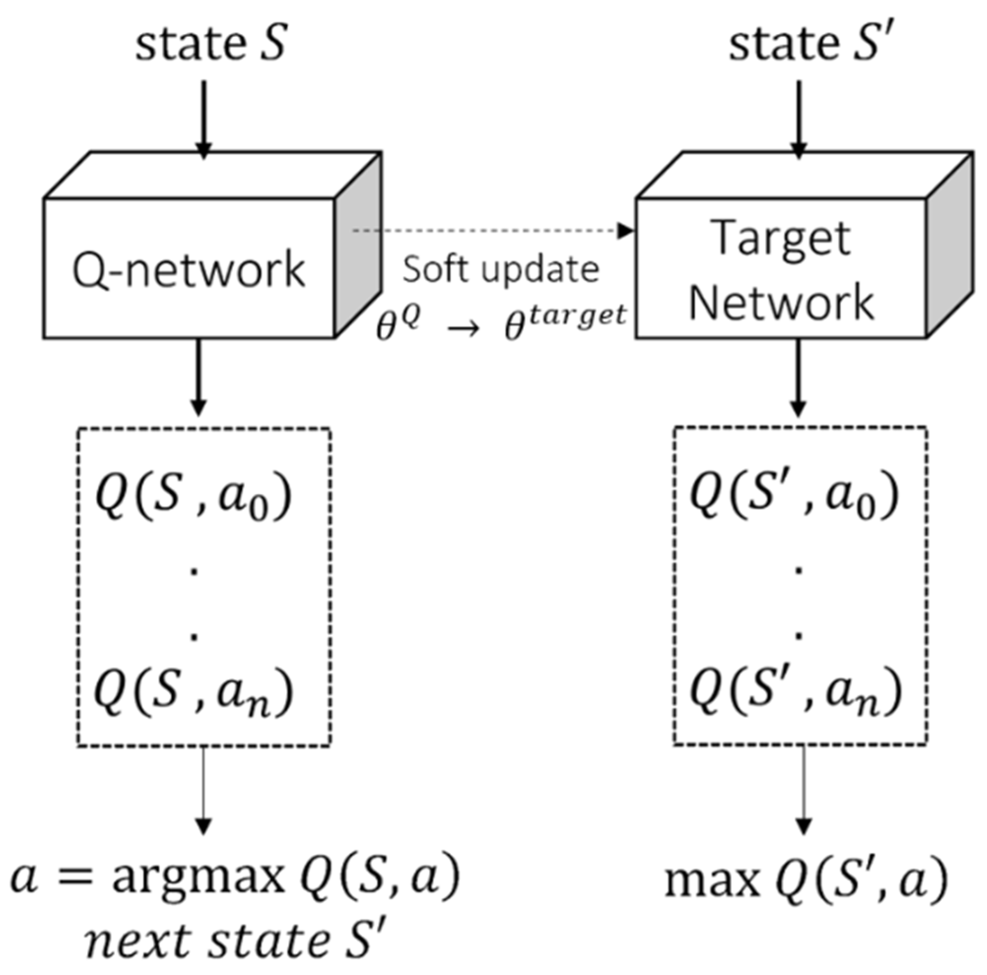
In order to calculate the Q-value, all rewards received after are demanded. According to the Q-learning algorithm, a two-dimensional matrix Q-table with as rows and as columns was introduced to record the Q-value of every combination of . Several numbers of simulations are required to update each of the Q-table. As mentioned above, (3) is calculated as the sum of (4) and the immediate reward; then, consequently, the Q-table is updated. The combination of state or action could be diversified; however, the size of the Q-table and the amount of computation will increase if there are many states and actions. To address these limitations, the DQN opened a new chapter in reinforcement learning with deep learning by devising the neural network Q-network to estimate Q-value [23]. For general deep learning tasks, input data are computed with the parameters of the neural network and passed through the activation layer; finally, it produces output data. Since output is the value predicted by the neural network, there is a target which the output of the neural network is supposed to attain. It is trained to update the neural network by back propagating the error between the target and the prediction in order that the output is close to the target. The entire system described above is referred to as deep learning. The input of the Q-network is state , and the output is the Q-value of each action in the action space. In (3), is calculated by the immediate reward and , which becomes the target of the Q-network. DQN learning is conducted through an error between and that is predicted as the Q-value by the Q-network. If in (3) was predicted through the Q-network, the target would change in every step. Due to the fixed target, this problem does not occur in supervised learning; however, in reinforcement learning, there is not a fixed target. Therefore, the learning might not be performed correctly only with the Q-network. The target network, which has the same structure as the Q-network and fixed weights, calculates and periodically copies weights of the Q-network; this is one of the characteristics of a double DQN (DDQN). As shown in Figure 1, copying weights of the Q-network is named as a soft update.
3. System Modeling
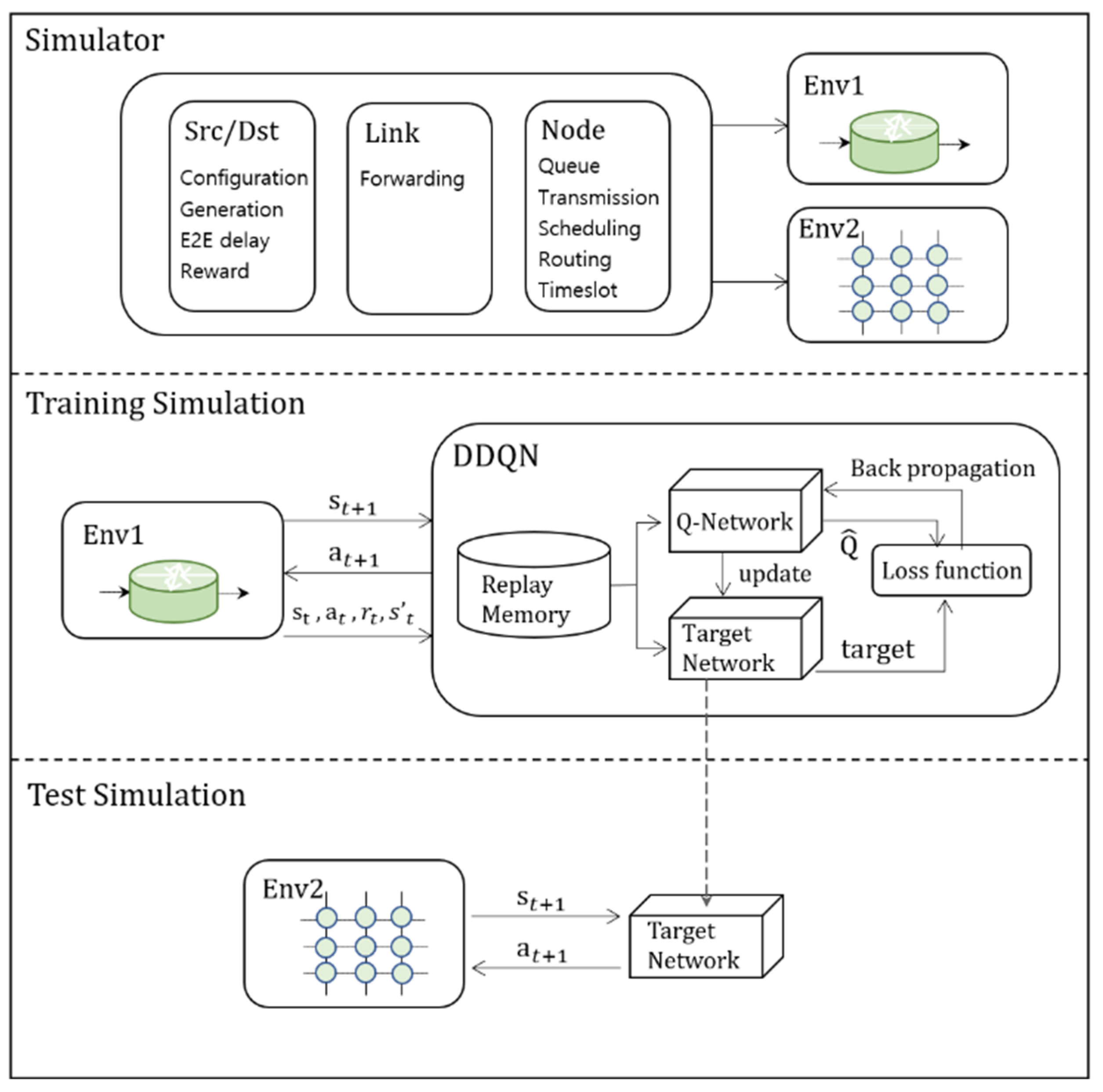
Figure 2 describes the proposed approach. The network simulation with deep learning requires customization of a simulator which reflects constraints of the network. We designed the elements of the network, such as the source, node, and link, to organize the environments.
3.1. Experiment Environment
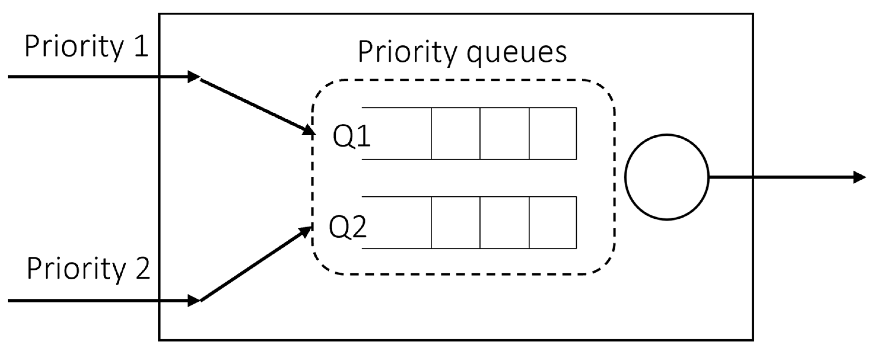
We designed a simple experiment environment in our study to find that reinforcement learning in timeslot scheduling is feasible. The structure of the output port of a switch node is shown in Figure 3. The DDQN agent is responsible for scheduling a timeslot of two priority queues in the node, and the output port is one. In this work, the agent was trained with only a simple experimental environment, and then evaluated by applying trained agents to mesh-type network topologies. Considering that it is a node on a network topology where many nodes exist, we introduced the number of remaining hops as each packet having to be sent when they arrive at the node, which is configured as a hyperparameter. A current delay denotes latency while the packet generated from the source arrives in the node. The current delay and remaining hop count are set to arbitrary values. All packets have a fixed size, and the size of a timeslot is equal to a packet size. Since our work configured the bandwidth to 20 Mbps and the size of the packet to 1500 bytes, the timeslot size would be 0.6 ms; i.e., a packet takes 0.6 ms to send to the next node. The packet arrival probability distribution is affected by the packet generation period, the number of flows, and the number of packets. In this study, we experimented with different numbers of packets and the period of packet generation for each of the two flows. In the training simulation environment of the DDQN, the number of packets is 40 for flow1 and 100 for flow2, and the period is the same as 1 timeslot. On the other hand, in the test simulation environment of the trained DDQN model, the number of packets is all equal to 60, and the generation period is equal to 2, or flow1 is allocated to 2 timeslots and flow2 is allocated to 4 timeslots. Hence, the three different packet generation and arrival patterns can be observed. When the number of packets in each flow is expressed as and the period is expressed as , the duration for packet generation can be expressed as . Then it could be generalized as follows, in which the subscript denotes priority of the flow.
Both priorities have deadlines to be met; every packet should arrive at its destination within the deadline, but there is a difference in their importance. The SP always serves a packet of high priority as long as the packet remains in the queue; therefore, occasionally low-priority packets cannot be transmitted within the deadline in situations with high utilization. Utilization is with respect to the transmission period of the packet. The shorter the generation period of packets using the link, the greater the utilization. Referring to Table 2 below, it may be seen that the arrival probability of priority 2 packets is lower than that of priority 1 packets. Thus, reinforcement learning was applied to schedule packets within the deadline according to their importance. In order for the reinforcement learning agent to implement optimal scheduling, it should delay high-priority packets a little and send more low-priority packets, but only to the extent that high-priority packets could satisfy the requirement. This is a point that emphasizes the need for reinforcement learning-based scheduling, with a need for algorithms that are required to operate very delicately and that must also change as the environment changes.
3.2. Application of DDQN
The DQN selects the best action in the current state through the Q-network. The Q-value approximation of the Q-network in DDQN derivation from (5) to (7) is summarized from [24]. is the output of the Q-network, and weights of the Q-network are expressed as . Equally, is an output using weights in the target network. The target can be expressed in (5). By calculating the square error of the target and , the error used in the learning can be obtained as shown in (6) below.
The Epsilon-greedy algorithm was used to increase the learning effect. The method uses the probability value , which gradually decreases from 1 to 0.01, to allow the agent to randomly select the action according to . Since decreases as episodes continue, the frequency of selecting the action that produces the maximum Q-value is increased. In this way, agents could establish the optimal policy and learn from various data. A tuple of is observed for each timestep and then stored in a replay memory buffer, and all data are divided into a mini-batch to proceed with the neural network’s learning. The replay memory buffer serves as a dataset of supervised learning, and a mini-batch consists of some samples acquired by the DDQN agent to efficiently train the neural network, as in supervised learning where the dataset is divided into batches. The DDQN has been proposed to solve the problem of overestimating Q-value in DQN or Q-learning [24]. By predicting a more accurate Q-value, our work achieved a stable arrival of a higher reward. The difference from the DQN is in calculating the target. In the case of the DQN, the action of the next state is selected only with , as shown in (5). On the other hand, the DDQN selects an action in the next timestep with and substitutes an output corresponding to the Q-value of the action selected with . This is expressed in the formula as shown in (7).
It is known that this could prevent propagation from occurring with an overestimated Q-value. Reinforcement learning should define the state, action, and reward to apply to the MDP problem of decision-making over discrete time. State, action, and reward are defined as in the following subsections, and symbols used to define the elements of reinforcement learning are described in Table 3.
- (1)
- State
The state should include the necessary information as concisely as possible but should represent all the situations that the environment needs to know. The agent could not have information about real E2E, which is essential to observe the state of the network. Thus, the state included ET information instead of real E2E. The current delay and the queueing delay of the packet are able to be observed. However, the delay of the packet from the single node to its destination cannot be observed in the single node. It takes a timeslot to transmit a packet in the timeslot-based environment; thus, ET has a unit of timeslot. The remaining hops and current delay are counted in units of timeslots as well. Since it can take exactly one slot for the packet to reach the next node, for remaining hops, it was assumed that the packet would be delayed as much as the remaining hops when estimating ET. The state denoted by is the set of the length of each queue and the maximum ET of packets in each queue, which changes according to timeslot .
- (2)
- Action
Because we assumed that one packet per timeslot can be transmitted, the choice of agent could be simplified to send a priority 1 or priority 2 packet at each timeslot. The agent selects an action of 0 or 1, where 0 means priority 1 packet transmission and 1 means priority 2 packet transmission.
- (3)
- Reward
Rewards should be set to induce behavior expected from reinforcement learning agents. Since the goal is to send as many packets as possible within the deadline, rewards if is less than . In the case of using only , it might happen that the agent does not send a packet, because it is expected to return the same reward as sending a packet over the deadline. To prevent this situation, always returns if the packet is sent, and parameter is set to be much smaller than and greater than zero. Consequently, the total reward at timeslot , , is defined as in the following equations. is defined to induce the agent to transmit as many packets as possible within the deadline while preserving weights of each priority, and is defined to prevent the agent from taking action not to transmit a packet if is not received.
4. Performance Evaluation
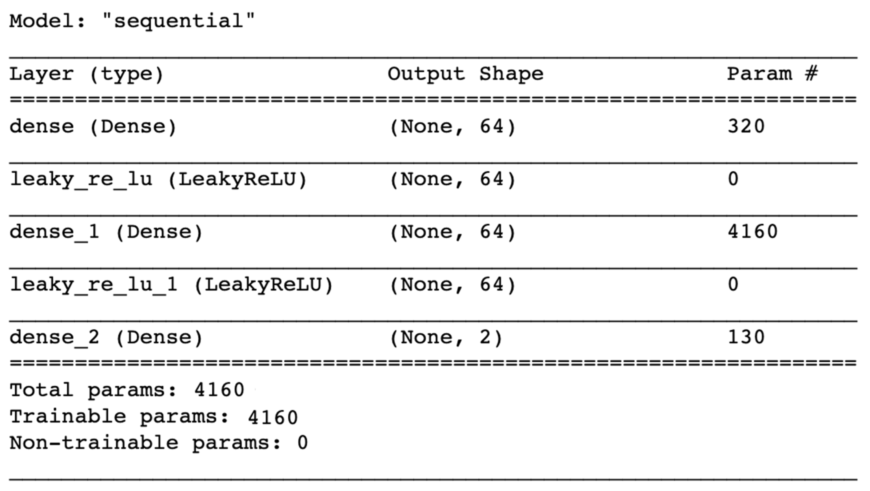
For the performance evaluation, we have implemented deep learning on the network using a discrete event-based simulation tool. A reinforcement learning simulation platform, Simpy, was used for our experiments [25]. For implementation of our simulator, the packet generation process and link, transport, source, and node are modularized with their processes. Training and tests are executed by interacting with the TensorFlow-based DDQN with the agent. The DDQN trains the outside of the simulation environment defined in Simpy; it does not affect the packet latency. In other words, training the DDQN results in delay due to inference and learning operations of the neural network, but the simulation environment does not take interference into account. However, in real-world network environments (i.e., where scheduling is required for every time slot), the delay of deep learning computation could occur. In preparation for this situation, the agent could select an action only with information about its own state, even if all switch nodes in the network were not known; it allows decentralization of the DDQN scheduler. The role of the trained DDQN is to output an optimal action by using the state as an input; the optimal action for the current state observed at the node could be recorded in the look-up table. The parameters set to train the DDQN are summarized in Table 4 on network simulation parameters and in Table 5 on the DDQN learning parameters. The structure of the DDQN can be seen in Figure 4. Linear was used for the activation function at the final output terminal, and Adam was used for the optimizer. This method uses an adaptive learning rate optimization algorithm, which is known to improve learning performance by updating weights using individual learning rates. In this study, the learning rate of was empirically determined based on the most effective value for loss reduction. The algorithms used for the result comparison are SP and WRR. SP is an algorithm that unconditionally sends packets in the highest priority queue. WRR is an algorithm that services queues sequentially in proportion to the weights allocated to each priority queue. In all simulations, including the DDQN, if a packet exists in only one priority queue, work-conserving was applied to send the packet regardless of the result of the scheduling.
4.1. Existing Algorithms
In this study, existing algorithms were used to objectively evaluate the performance of the DDQN agent. As mentioned in Section 3 some packets could not arrive within the deadline in situations where utilization increases due to the sudden influx of packets into the link. Table 2 confirms that existing algorithm SP has weaknesses that are difficult to adaptively respond to. Unlike SP, which unconditionally gives preemption to high priority, WRR can perform more flexible scheduling than SP in that it can assign weights to each queue. Work-conserving has been applied to all algorithms, including SP, WRR, and DDQN agents, to ensure that packets are sent when they are waiting. For instance, if packets exist in only one of the two queues, they are sent immediately without using the scheduling algorithm. Not only did this meet the requirements of the packet, but it also helped reduce the running time. WRR allows the allocated weights to be involved only when packets exist in both queues; in other words, when it has a weight of 3:1, it means transmission of three priority 1 packets and one priority 2 packet only by scheduling without work-conserving. The weight is set according to the network situation; even in the same situation, the result might vary depending on the weight. Therefore, for each simulation below, an indicator for evaluating the performance according to the weight of the WRR is added.
4.2. DDQN Training Results
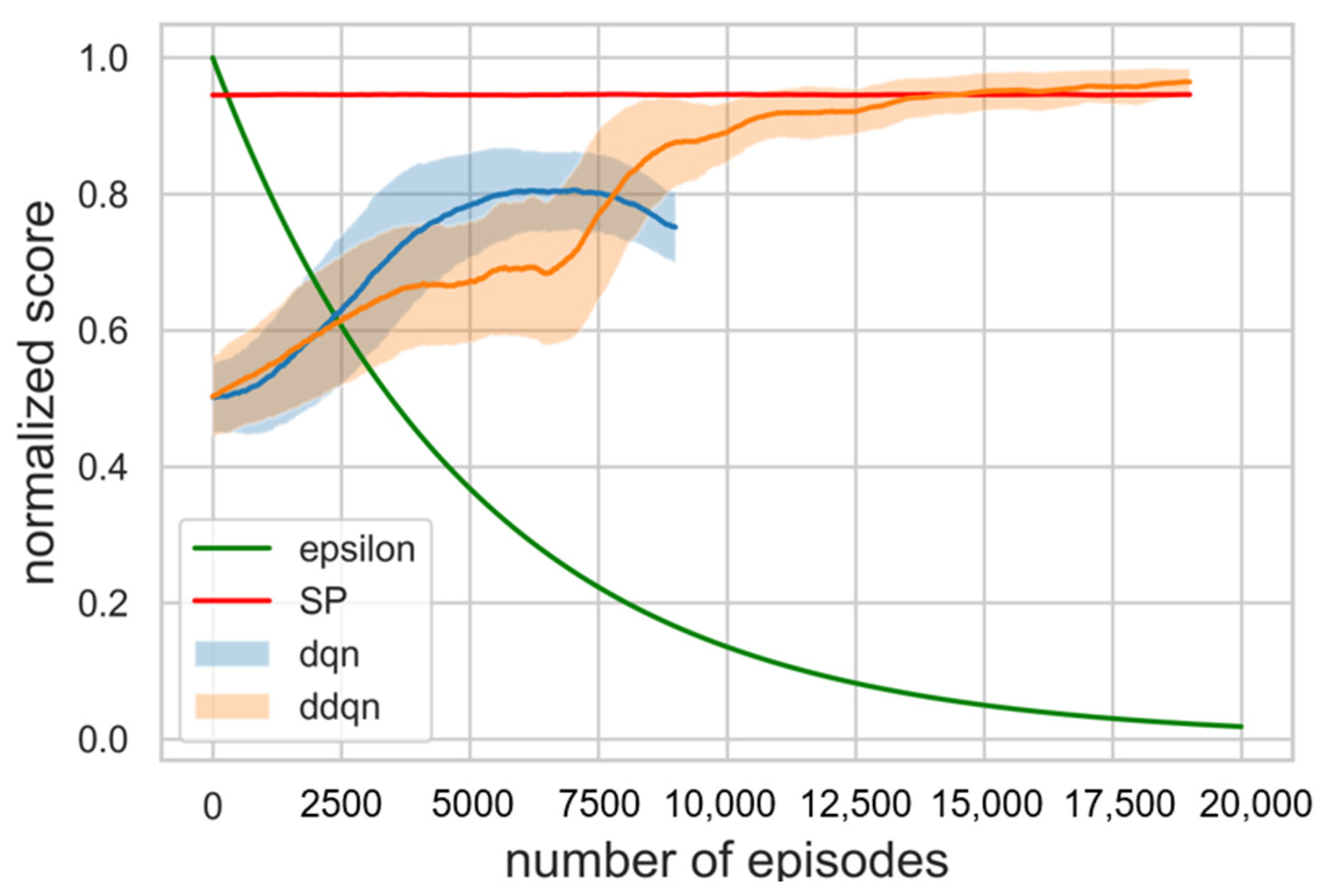
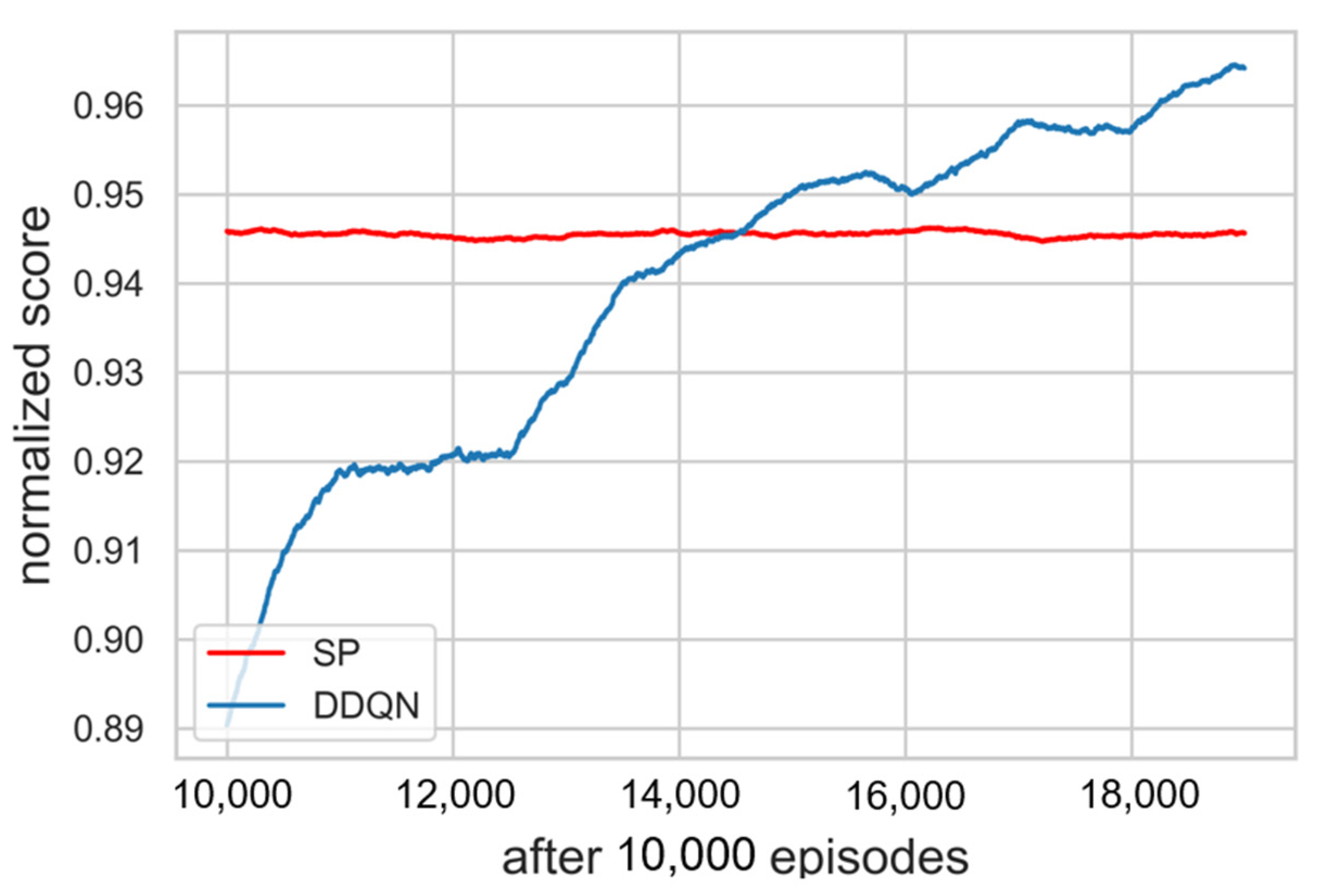
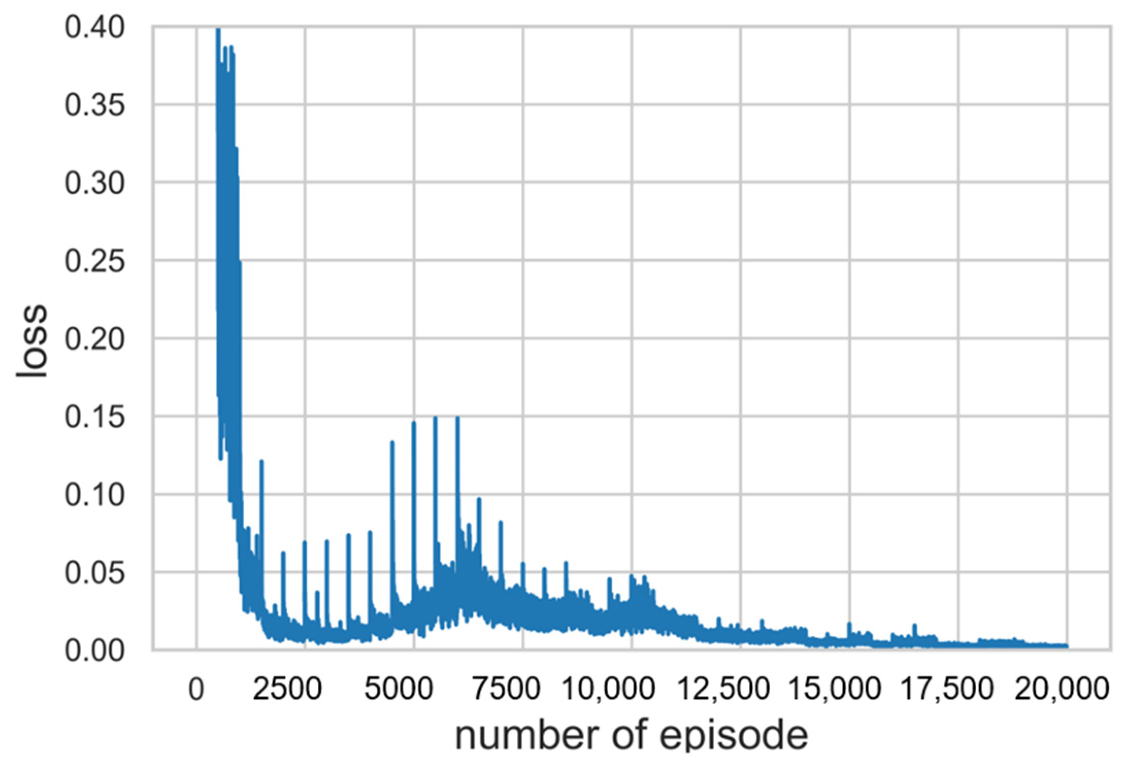
As a result of training for hyperparameter tuning, it was confirmed that the higher the value assigned to priority 1, the better the performance that was shown. Β should have less effect than α and greater than 0, so a value of 0.01 was assigned. Figure 5 is a learning curve comparing the results of DDQN training with 20,000 episodes, DQN training with 10,000 episodes, and SP simulation in 20,000 episodes. The moving average of the DQN learning curve showed a continuous decrease, and we stopped the training early because we decided that there was no possibility of improvement. The cumulative sum of rewards, which is specified as a score obtained in each timestep of an episode, was used as the result indication. The moving average of the score with window size 1000 and the moving standard deviation with the range of 30% transparency were exploited to display the learning curve. Each score was normalized to a range between 0 and 1 by adjusting the score with the max value in the episode. As ∈ decreased, the score of the DDQN increased and learning was progressing properly. Referring to Figure 6, the score of the DDQN was recorded higher as compared with existing algorithm SP after 15,000 episodes. It was confirmed that the loss function gradually converges close to zero as well. As mentioned above, loss function is used to optimize neural network parameters and we define it to be MSE (Mean Square Error), which is applied to measure and improve the accuracy of prediction. It is a partial derivative with respect to the parameters, then back propagated to update them. Hence, a decrease of loss denotes that the criterion of accuracy has been improved through iterations of training. The progress of loss during episodes is shown in Figure 7.
4.3. Single Node Simulations
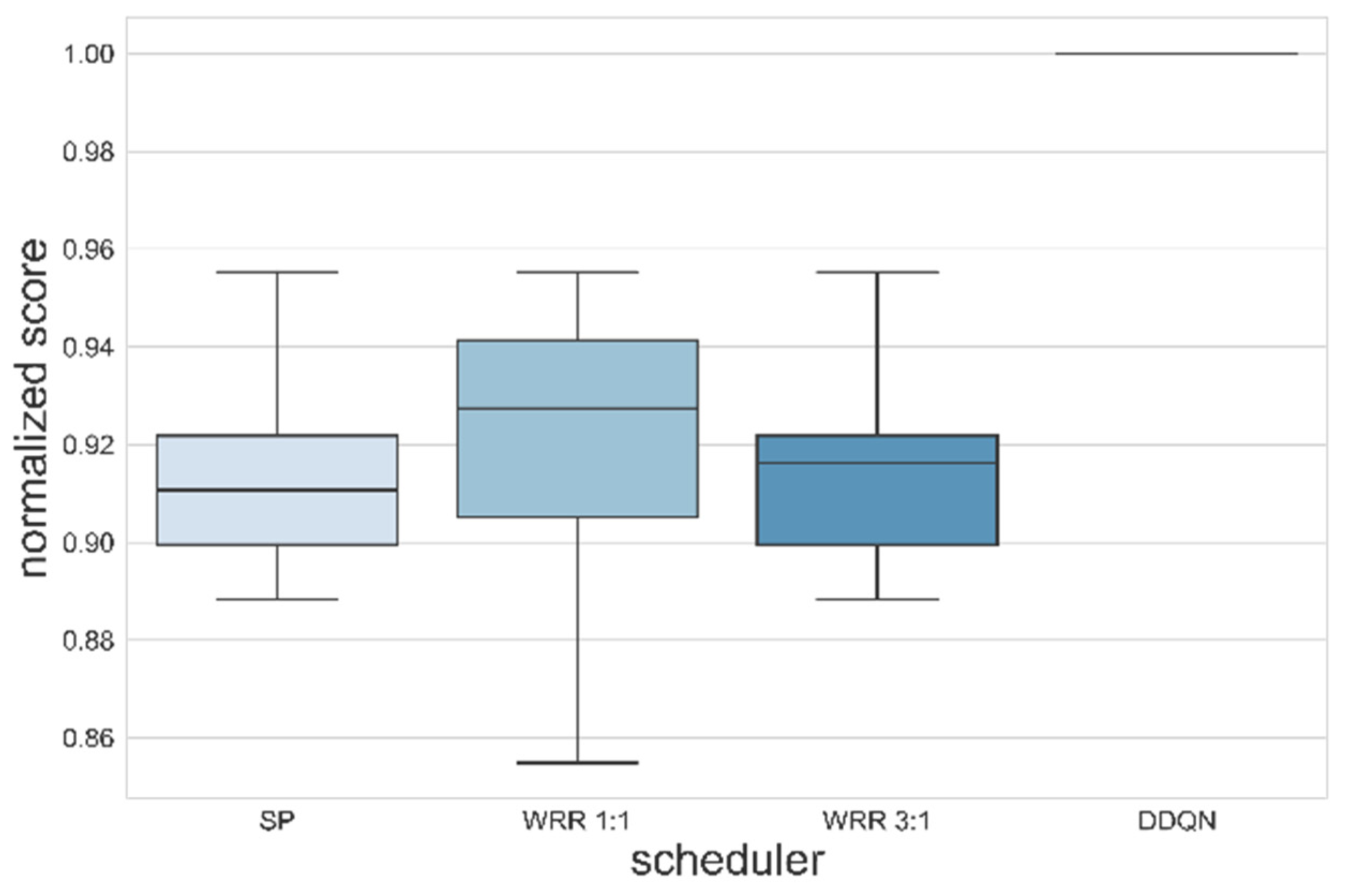
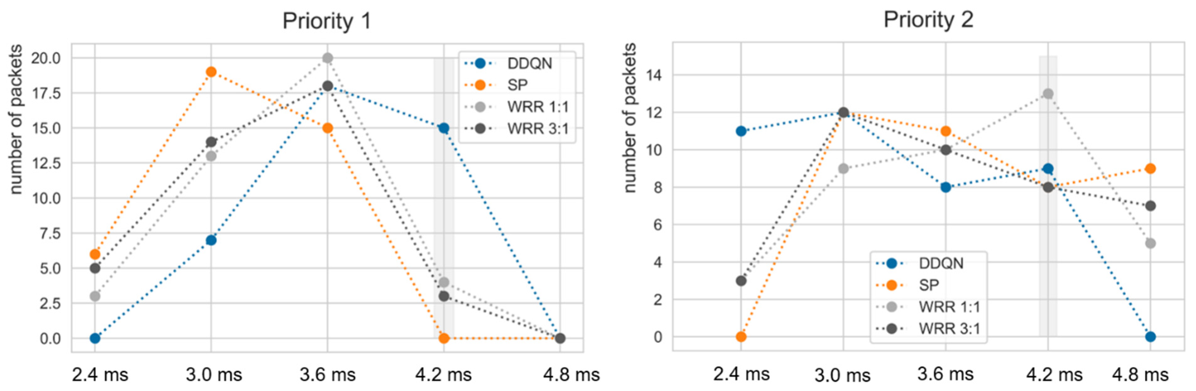
The training was successfully performed in the single node that has the output port structure shown in Figure 3. Simulations were conducted under the same environmental variables as the existing algorithm by applying a trained agent for evaluation. Figure 8 indicates the comparison between the trained deep learning model and the existing algorithms. All algorithms were tested 10 times; thus, the distribution of data could be considered. Unlike the environment of DDQN learning, with 200% of maximum link utilization (i.e., priority 1 and priority 2 packets generated at a period of 1 timeslot), all packet generation periods were set to 2 timeslots and tested. The deadlines of all flows were fixed at 7 timeslots, and the packet number of each flow was set to 40. The current delay was designed considering remaining hops since we assumed that packet has a smaller remaining hop means packet was sent from source longer timeslots ago. As could be seen from Figure 8, the trained DDQN achieved 100% of a normalized score even though parameters were changed, proving that it would adapt well to dynamic environments. On the other hand, the existing algorithms remained in average performance at around 90%~92%. This result suggests that the DDQN could guarantee deadline requirements for more packets in timeslot scheduling with priority unlike other algorithms. SP and WRR showed similar normalized scores. WRR, with a weight of 1:1, showed higher average performance than WRR at 3:1. Table 6 shows the results of deadline satisfaction according to weight in the same network environment. Since the period ratio of each priority is 1:1, the weight also achieved a higher satisfaction rate as it is closer to 1:1; however, it could not achieve more than 90% in priority 2. In order to confirm whether a deadline is guaranteed or not for every flow (i.e., to confirm the accomplishment of the purpose of our work), the delay for each algorithm and priority was confirmed in Figure 9. The gray area denotes the deadline. As we assumed that the agent utilizes ET, it is impossible to find the real E2E of packets. The timeslot is 0.6 ms and the deadline is 4.2 ms; thus, the deadline is 7 timeslots. In the simulation environment, as the packet arrival is constant, the length of the queue is increased. Accordingly, since packets transmitted at the beginning of the packet generation process have a small ET, and packets transmitted later have a larger ET, some fluctuation of the number of packets may occur. The ET of priority 1 was slightly increased but the ET of priority 2 was slightly decreased, so that all packets arrived within the deadline, contrary to other algorithms. Therefore, the simulation results in a single node might be interpreted as an accomplishment of the purpose and intention of the training DDQN agent.
4.4. Simulations in Network Topology
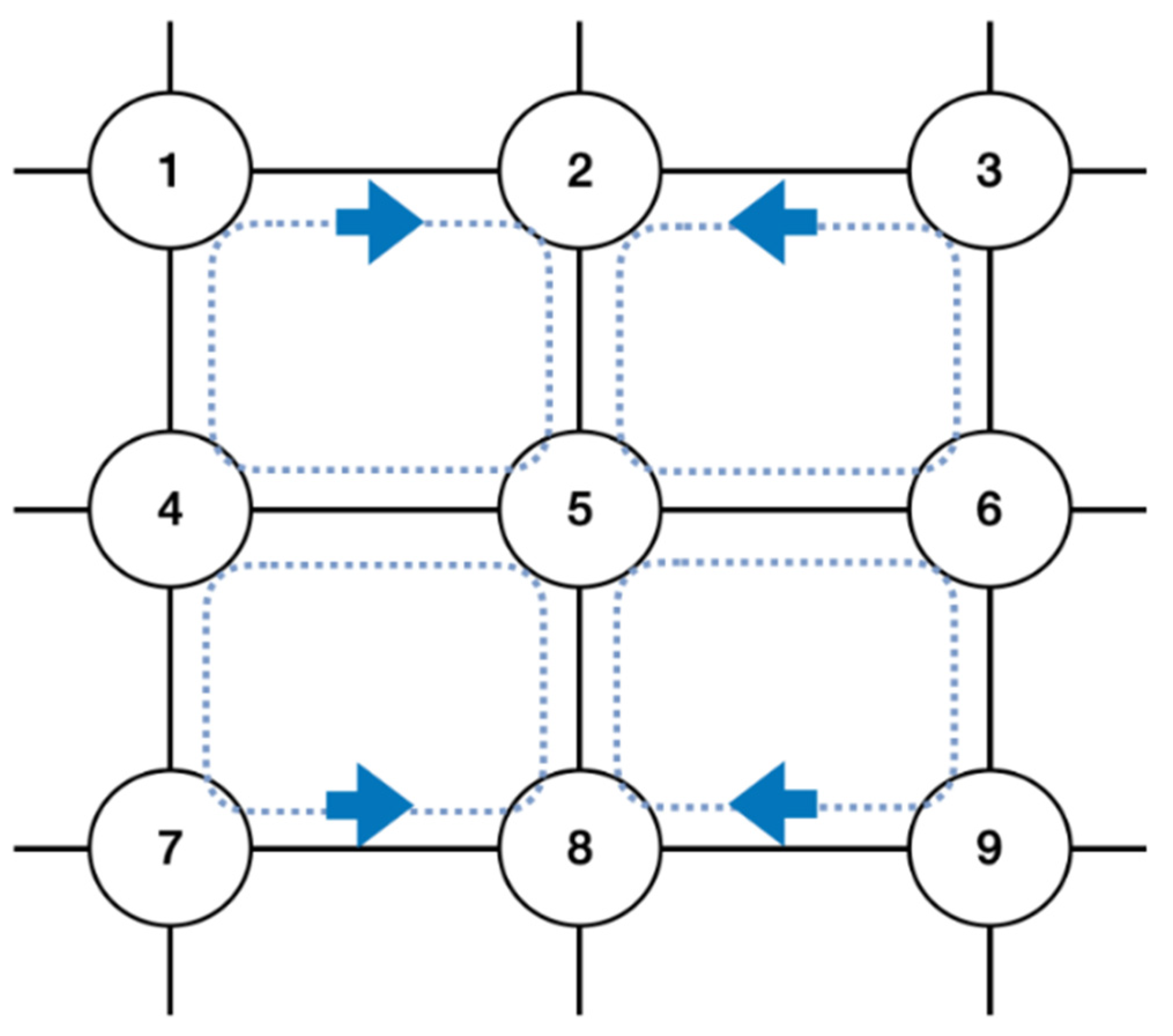
In Section 4.2, it was confirmed that the DDQN operates in various parameters in the single node environment. We implemented a well-known mesh-type network topology with nine nodes, as shown in Figure 10 [16,26], in order to verify that the DDQN scheduler works properly even when expanding the network size, and then applied the same trained model for comparison of the performance of the scheduling algorithms and analysis of delay. We used ET when training on a single node, but there is no way to observe whether the DDQN agent correctly estimated the E2E. Hence, we measured that simulation in the network topology is also essential. In the topology, each node delivers the state to a trained DDQN agent, which is assumed to be embedded inside of each node and receive the action. Because the state defined as an MDP problem is independent, the entire network situation is unknown to other nodes. Therefore, the key of our work is that scheduling is properly performed with ET through topology simulation. If the information of another node is added to the state, scheduling performance could be improved, but the state-space would be vast, resulting in a large amount of computation, and as the node is added, it will be difficult to apply. We conducted a simulation on various scenarios which are set with eight flows and two priorities. The eight flows are shown in Table 7, and the route is the sequence of nodes through which the flow passes. The number of nodes is the same as in Figure 10. The first index is the node connected to the source, and the last index is the node connected to the destination. Each node of the topology has two input ports and two output ports. The structure of the output port defined in Figure 3 is applied, which means that there are two priority queues per port. Scheduling is performed on a per-port basis, and as mentioned, the scheduling algorithm operates only when packets are simultaneously queued in two priority queues. In particular, if the flows defined in Table 7 share the same link, the scheduling algorithm is applied instead of work-conserving; The link from node 2 to node 5 is shared by F1 and F2, and the link from node 8 to node 5 is shared by F7 and F8. Therefore, the simulation can be conducted with only F1, F2, F7, and F8. Our proposed DDQN-based timeslot scheduling process is described in Algorithm 1.
| Algorithm 1 DDQN scheduling simulation in topology |
| N = number of nodes in topology P = number of priority queues in a port of a node = 2 Init priority_queues [1..P] Init action[1..N], state[1..N], next_state[1..N], reward[1..N], timeslot DDQN trained_ddqn_weights while not done : timeslot += 1 for each SourceModule do: SourceModule.PacketGeneration if timeslot : # not initial timeslot for n in 1..N: state[n] next_state[n] if any NodeModule[n].Queues is not empty: action[n] DDQN.ChooseAction else: action[n] NodeModule[n].WorkConserving for n in 1..N: packet NodeModule[n].Scheduling(action[n]) priority_queues[P] packet #the priority of the packet is P NodeModule[n].Send(priority_queues[P]) next_state[n] NodeModule[n].StateObserve if transmission terminated: done = True return |
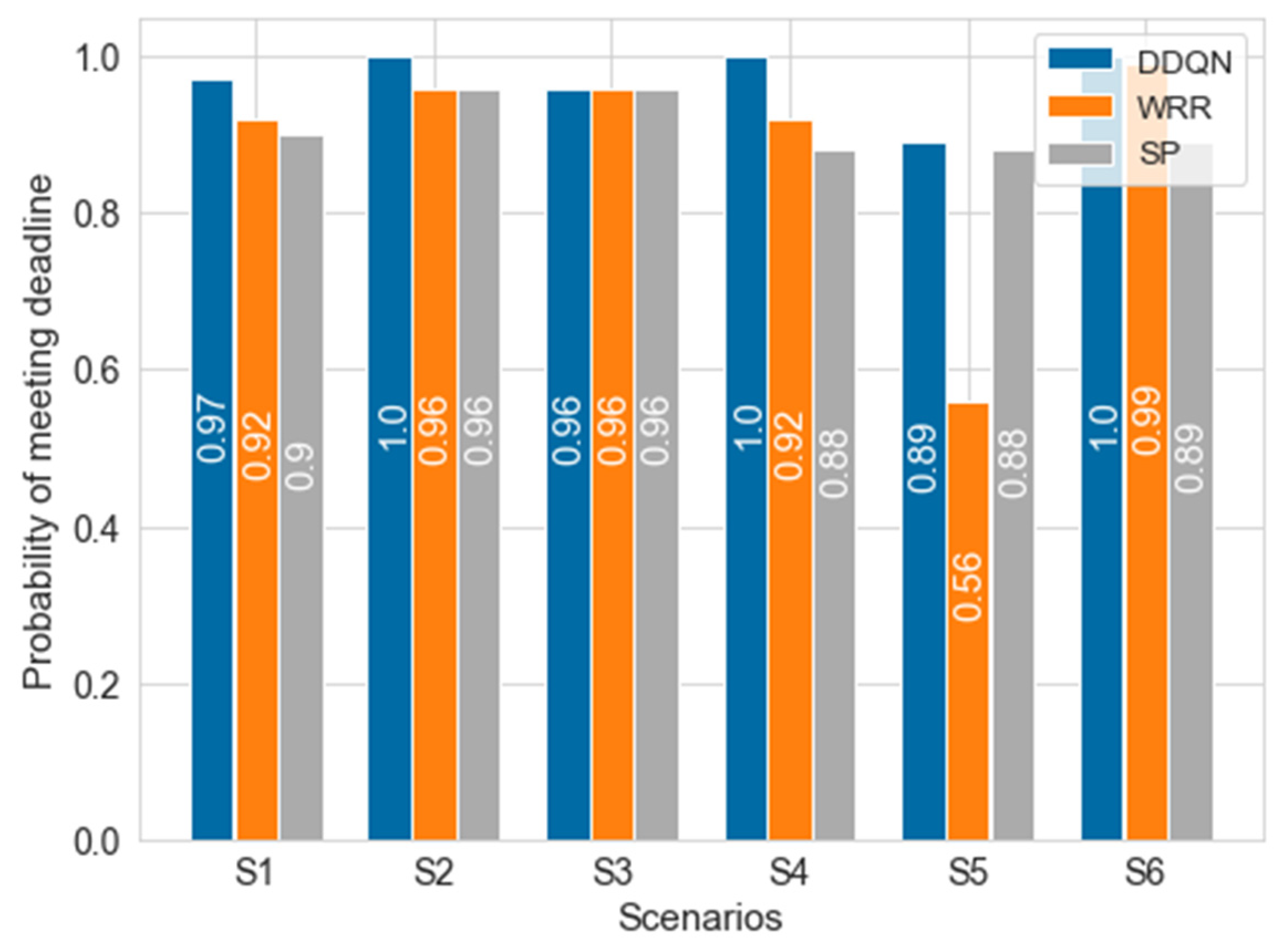
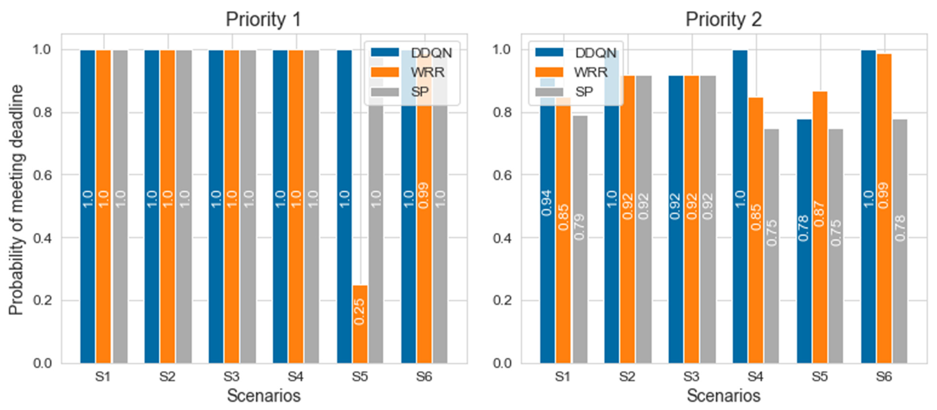
In Table 8 below, there are six scenarios where we experimented. The deadline and period are represented by tuples for priority 1 and 2, respectively, and T means timeslot. The probability of meeting the deadline of the DDQN, SP, and WRR in simulations of each scenario are shown in Figure 11 and Figure 12. There are scenarios in which the model trained from the single node using ET shows 100% deadline meeting, and the DDQN performance is higher overall. In the case of SP, 100% of the deadline was met for priority 1, but the deadline for priority 2 is not perfectly guaranteed. In the case of WRR, if the packet generation period is longer than two slots due to work-conserving, scheduling is similar to that of SP. Since it has a weight of 3:1, it shows a low probability of meeting deadlines in an environment such as S5, where the packet generation period is different from its weight’s inverse proportion. This means that when using WRR, the weight must also be changed according to the changing environment. In the case of the proposed DDQN scheduler, the results have been demonstrated to successfully address the drawback of SP and WRR.
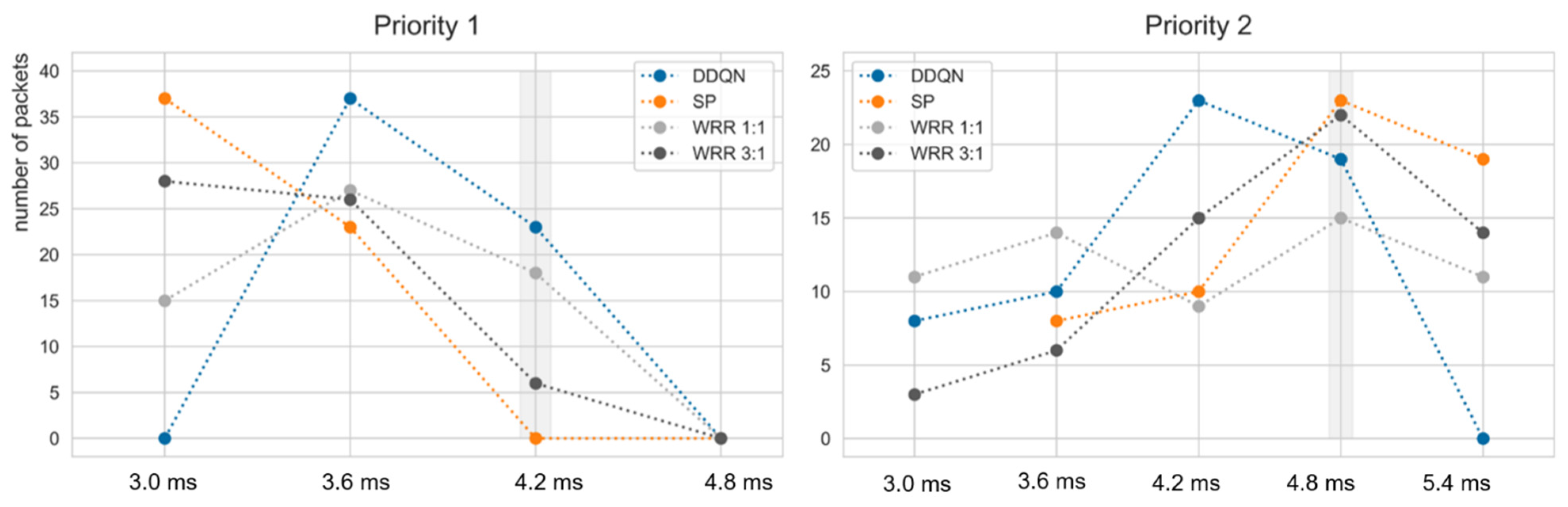
Table 9 denotes the results of deadline meets according to weight at scenario S4. In S4, since each period of priority is 2T, it shows the highest satisfaction at a weight of 1:1. Among the S1 to S6, WRR showed especially poor performance in S5. This shows that the weight of the WRR is sensitive to the maximum utilization (i.e., period of the packet). In Table 10, the WRR results according to the weight of S5 may be confirmed. Since S5 has periods of 1T and 5T, respectively, it is an environment with high utilization of up to 120%. This demonstrated the more weight needing to be assigned to the packet having the shorter period. However, this is slightly lower than that of the DDQN, and there is a disadvantage that WRR weight must be reassigned when the utilization changes. In Figure 11, the E2E in the DDQN, SP and WRR was illustrated. It was confirmed that every packet scheduled by the DDQN arrived within the deadline. The left graph of Figure 11 corresponds to flow F1 and the right graph corresponds to F2, and the graphs mean the E2E of 60 packets in scenario S4.
The x-axis represents the E2E in ms instead of the timeslot unit. Figure 13 might imply why it could substantially improve the performance. Scheduling algorithms including the DDQN transmitted high-priority packets within the required deadline, but the DDQN transmitted more low-priority packets compared to other existing algorithms. It can be seen that the trained DDQN agent takes action to transmit low-priority packets while delaying high-priority packets to a limit where the packets can be transmitted within the deadline. In contrast, the SP and WRR algorithms transmit many high-priority packets even though there are many deadlines left, so it can be seen that low-priority packets are delayed. This also can be observed in Figure 9 and Figure 13. Although the research results demonstrate that DRL shows potential for network scheduling, several challenges remain: reinforcement learning agents should be generalized so that the agents do not operate only in the environment configured in the simulation, and the computational complexity should be reduced so that DRL can be applied to network equipment.
4.5. Simulations in Network Topology
As mentioned in Section 1, there is a problem of deep learning inference time as a task to be solved in order to apply DRL to networks. In this study, in an effort to reduce the inference time, inference at every timeslot is prevented through work-conserving, and single nodes can independently act without correspondence with the central node. Despite it being designed this way, the action is still chosen by the agent; and it takes considerable computation time. We designed the simulation not to consider the deep learning inference time, but it is difficult to do this in real situations. Therefore, we have introduced a table look-up method as a simple way to reduce inference time. This means all observed states and actions in multiple times of simulation are stored in a look-up table, and the simulation with a look-up table is performed with the table look-up method instead of the DDQN. When it uses the table look-up method, the action of the next timeslot is decided by searching the state from the look-up table, avoiding the computation of the DDQN. If a state does not exist in the look-up table, it operates as an SP algorithm. Because of the simulation in the same scenario, the rate at which packets arrive within a deadline is very similar to the DDQN results in Figure 12, but the inference time is significantly reduced, as shown in Table 11 below; for example, in Scenario 1, the simulation time of the look-up table is approximately 1.4/100 of the DDQN time. This suggests the possibility that if the model is trained, the inference can be partially replaced by the table look-up method; also, it can be expected that reinforcement learning can be introduced in small networks by distributing only simplified tables without having to periodically distribute models after training all newly observed samples at the central processing node. However, the disadvantage of this method is that the agent needs to know the state and action possible for all scenarios, and that it can only choose one predetermined action for the state. As a solution to this, a policy-distillation method for reducing the computation of reinforcement learning can be considered [27]. Policy distillation is a technique that lessens the computation by transferring a teacher model, where training is actually done, to a small student model. Policy-distillation has shown that the computational time is very low, and the student’s performance can be close to that of the teacher. In fact, there has been a discussion in [4] that the implementation problem of deep learning in networks can be solved through policy transfer learning of policy distillation. In addition, in [10], policy distillation was applied as a way to output real-time tasks in microseconds to replace existing congestion control algorithms in C-RAN with DRL. In the study, policy was transferred to a decision tree of appropriate depth that achieves performance similar to the original model and negligible inference time. The proposed model based on the DDQN is trained in every timeslot. The experience replay keeps repeating while training. As a result, the learning slows down, and the complexity increases as the learning progresses due to the accumulation of observed data samples. To address these issues, we tried to exclude unnecessary experience and deep learning inference. Timeslot data that are not needed during training (e.g., state elements are all 0 and no packets are generated at a timeslot) are not added to memory. In addition, when there are packets in only one of Queue 1 or Queue 2, the experience replay is not required, so it is excluded from replay memory. This could make it possible to not significantly slow down.
5. Conclusions
This study proposed timeslot scheduling based on deep reinforcement learning. Reinforcement learning with deep learning has been known as an algorithm that reduces computational time and increases Q-value prediction performance compared to Q-learning. With deadlines also required for traffic of lower priority, we hypothesized that more packets would be sent within deadlines if the higher priority yielded a timeslot to the lower priority at an appropriate state. The DDQN agent was conducted to reward when the ET of the packet was less than the deadline. After about 15,000 episodes, the score of the DDQN showed that it outperformed SP on the learning curve. As a result of simulation under the environment of utilization smaller than the learning environment, SP or WRR recorded a score of 90% and the DDQN recorded a score of 100%. This means that the DDQN could guarantee more packet deadlines than existing algorithms. Furthermore, in the results of testing by expanding the network structure, the DDQN always performed higher or the same while improving the weaknesses of other algorithms. The E2E of packet scheduling with the DDQN was validated to be adjusted in order to meet the deadline. Reinforcement learning would provide optimal scheduling to meet the requirements of networks where vast amounts of data are transmitted without intervention of an administrator, and be able to reach the goal of autonomous networking that responds immediately to changes in the network environment. This study has shown the feasibility of introducing deep learning into future intelligent networks. We are planning to develop a well-adapted agent to a more dynamic network environment for a generalized reinforcement learning scheduler. The essential factors of future work are defining different priorities and classes of flows, and being robust for various utilization and requirements. In addition, we are planning to devise a solution for reduction of operation, such as a policy-distillation method to reduce inference time, aiming for DRL in the network to be applied in a real case. In order to apply the deep learning modules in PyTorch or TensorFlow, we implemented our Simpy-based simulation, and not use other network simulation frameworks. Hence, it makes deep learning difficult to be accepted in networking. In order to apply a deep learning model based on Python to a network, most of the related research developed the simulator independently, which is able to be employed on their work only [28]. Therefore, the simulator should be standardized so that various environments and models can be tested and compared. In order to develop deep learning-based networks, it will be directed to improve DRL scheduling performance, which remains a challenge, as well as to build standardized simulators and benchmark datasets.
Reinforcement learning-based network scheduling is still in its early stage. Although the DDQN agent in this paper showed better performance than the existing algorithms, the following limitations are remaining. We also suggest future work to solve these limitations.
(1) Generalization and robustness issues: In this study, priority-based scheduling is performed in a simplified timeslot environment. However, real traffic patterns and network conditions can be more complex. We expect the scheduler performance would be different according to such discrepancies in more realistic environments. Therefore, in subsequent studies, the flow configurations will reflect better the real-word traffic, and network topologies and sizes will reflect the real networks. We also plan to compare the results in diverse aspects and analyze the agent’s policy. In addition, various DRL models will be explored and simulated and compared in terms of efficiency and performance.
(2) Scalability issues: Limitations on computing resources make it difficult to realize the suggested framework in real implementations. In subsequent studies, a more scalable approach will be employed, in which the central node distributes a lightweight model (for example, policy distillation), and the other nodes use the lightweight model to reduce complexity in terms of computation and memory.
(3) Bias issues: The evaluation results shown in this work may have been biased. Since the simulator was developed by itself and was executed only in a network environment where conditions were set, it is necessary to compare the results in various aspects and analyze the agent’s behavior to give objectivity. It is possible to enhance the proposed framework by modifying the inference frequency and the system input/output.
Author Contributions
Conceptualization, J.R., T.C. and J.J. and J.K.; methodology, J.R., T.C. and J.K.; software, J.R and J.K.; validation, J.J., J.R., T.C. and J.K.; formal analysis, J.J. and J.-D.R.; investigation, T.C. and J.-D.R.; writing—original draft preparation, J.R.; writing—review and editing, J.J., T.C. and J.-D.R.; visualization, J.K.; supervision, J.J.; project administration, J.J. and J.-D.R.; funding acquisition, J.J. and T.C. All authors have read and agreed to the published version of the manuscript.
Funding
This work was supported by an Electronics and Telecommunications Research Institute (ETRI) grant funded by the ICT R&D program of Korea Government (MSIT/IITP) [2021-0-00715, Development of End-to-End Ultra-high Precision Network Technologies].
Conflicts of Interest
The authors declare no conflict of interest.
References
- Zhang, C.; Patras, P.; Haddadi, H. Deep learning in mobile and wireless networking: A survey. IEEE Commun. Surv. Tutor. 2019, 21, 2224–2287. [Google Scholar] [CrossRef] [Green Version]
- Cheng, Y.; Yin, B.; Zhang, S. Deep learning for wireless networking: The next frontier. IEEE Wirel. Commun. 2021, 28, 176–183. [Google Scholar] [CrossRef]
- Mao, Q.; Hu, F.; Hao, Q. Deep learning for intelligent wireless networks: A comprehensive survey. IEEE Commun. Surv. Tutor. 2018, 20, 2595–2621. [Google Scholar] [CrossRef]
- Nguyen, C.T.; Van Huynh, N.; Chu, N.H.; Saputra, Y.M.; Hoang, D.T.; Nguyen, D.N.; Pham, Q.V.; Niyato, D.; Dutkiewicz, E.; Hwang, W.J. Transfer learning for future wireless networks: A comprehensive survey. arXiv 2021, arXiv:2102.07572. [Google Scholar]
- Chinchali, S.; Hu, P.; Chu, T.; Sharma, M.; Bansal, M.; Misra, R.; Pavone, M.; Katti, S. Cellular network traffic scheduling with deep reinforcement learning. In Proceedings of the Thirty-Second AAAI Conference on Artificial Intelligence, New Orleans, LA, USA, 2–7 February 2018. [Google Scholar]
- Xiong, X.; Zheng, K.; Lei, L.; Hou, L. Resource allocation based on deep reinforcement learning in IoT edge computing. IEEE J. Sel. Areas Commun. 2020, 38, 1133–1146. [Google Scholar] [CrossRef]
- Chilukuri, S.; Pesch, D. RECCE: Deep reinforcement learning for joint routing and scheduling in time-constrained wireless networks. IEEE Access 2021, 9, 132053–132063. [Google Scholar] [CrossRef]
- Mollahasani, S.; Erol-Kantarci, M.; Hirab, M.; Dehghan, H.; Wilson, R. Actor-Critic Learning Based QoS-Aware Scheduler for Reconfigurable Wireless Networks. IEEE Trans. Netw. Sci. Eng. 2021, 9, 45–54. [Google Scholar] [CrossRef]
- Zheng, T.; Wan, J.; Zhang, J.; Jiang, C. Deep reinforcement learning-based workload scheduling for edge computing. J. Cloud Comput. 2022, 11, 1–13. [Google Scholar] [CrossRef]
- Martins, J.P.; Almeida, I.; Souza, R.; Lins, S. Policy Distillation for Real-Time Inference in Fronthaul Congestion Control. IEEE Access 2021, 9, 154471–154483. [Google Scholar] [CrossRef]
- Behringer, M.; Pritikin, M.; Bjarnason, S.; Clemm, A.; Carpenter, B.; Jiang, S.; Ciavaglia, L. Autonomic Networking: Definitions and Design Goals; No. rfc7575; RFC Editor: Fremont, CA, USA, 2015. [Google Scholar]
- Shin, S.J.; Yoon, S.H.; Lee, B.C.; Kim, S.G. Trends in Autonomic Networking Research. Electron. Telecommun. Trends 2017, 32, 25–34. [Google Scholar]
- Lei, L.; Tan, Y.; Zheng, K.; Liu, S.; Zhang, K.; Shen, X. Deep reinforcement learning for autonomous internet of things: Model, applications and challenges. IEEE Commun. Surv. Tutor. 2020, 22, 1722–1760. [Google Scholar] [CrossRef] [Green Version]
- Ayoubi, S.; Limam, N.; Salahuddin, M.A.; Shahriar, N.; Boutaba, R.; Estrada-Solano, F.; Caicedo, O.M. Machine learning for cognitive network management. IEEE Commun. Mag. 2018, 56, 158–165. [Google Scholar] [CrossRef]
- Time-Sensitive Networking Task Group. Available online: https://www.ieee802.org/1/pages/tsn.html (accessed on 18 February 2023).
- Joung, J.; Kwon, J. Zero jitter for deterministic networks without time-synchronization. IEEE Access 2021, 9, 49398–49414. [Google Scholar] [CrossRef]
- Xue, Y.; Gedo, C.; Christou, C.; Liebowitz, B. A framework for military precedence-based assured services in GIG IP networks. In Proceedings of the MILCOM 2007-IEEE Military Communications Conference, Orlando, FL, USA, 29–31 October 2007; IEEE Press: New York, NY, USA, 2008; pp. 1–7. [Google Scholar]
- Zewde, T.A.; Gursoy, M.C. NOMA-based energy-efficient wireless powered communications. IEEE Trans. Green Commun. Netw. 2018, 2, 679–692. [Google Scholar] [CrossRef] [Green Version]
- Fang, Z.; Wang, J.; Ren, Y.; Han, Z.; Poor, H.V.; Hanzo, L. Age of information in energy harvesting aided massive multiple access networks. IEEE J. Sel. Areas Commun. 2022, 40, 1441–1456. [Google Scholar] [CrossRef]
- Ghosal, D.; Shukla, S.; Sim, A.; Thakur, A.V.; Wu, K. A reinforcement learning based network scheduler for deadline-driven data transfers. In Proceedings of the 2019 IEEE Global Communications Conference (GLOBECOM), Waikoloa, HI, USA, 9–13 December 2019; IEEE Press: New York, NY, USA, 2020; pp. 1–6. [Google Scholar]
- Wei, H.; Zheng, G.; Yao, H.; Li, Z. Intellilight: A reinforcement learning approach for intelligent traffic light control. In Proceedings of the 24th ACM SIGKDD International Conference on Knowledge Discovery & Data Mining, London, UK, 19–23 August 2018; Association for Computing Machinery: New York, NY, USA, 2018; pp. 2496–2505. [Google Scholar]
- Zheng, G.; Zang, X.; Xu, N.; Wei, H.; Yu, Z.; Gayah, V.; Xu, K.; Li, Z. Diagnosing reinforcement learning for traffic signal control. arXiv 2019, arXiv:1905.04716. [Google Scholar]
- Mnih, V.; Kavukcuoglu, K.; Silver, D.; Graves, A.; Antonoglou, I.; Wierstra, D.; Riedmiller, M. Playing atari with deep reinforcement learning. arXiv 2013, arXiv:1312.5602. [Google Scholar]
- Van Hasselt, H.; Guez, A.; Silver, D. Deep reinforcement learning with double q-learning. In Proceedings of the AAAI Conference on Artificial Intelligence 2016, Phoenix, AZ, USA, 12–17 February 2016; AAAI Press: Palo Alto, CA, USA, 2016; Volume 30. [Google Scholar]
- SimPy. Readthedocs. Available online: https://simpy.readthedocs.io/en/latest/ (accessed on 13 November 2022).
- Joung, J.; Kwon, J.; Ryoo, J.D.; Cheung, T. Asynchronous Deterministic Network Based on the DiffServ Architecture. IEEE Access 2022, 10, 15068–15083. [Google Scholar] [CrossRef]
- Rusu, A.A.; Colmenarejo, S.G.; Gulcehre, C.; Desjardins, G.; Kirkpatrick, J.; Pascanu, R.; Mnih, V.; Kavukcuoglu, K.; Hadsell, R. Policy distillation. arXiv 2015, arXiv:1511.06295. [Google Scholar]
- Kherbache, M.; Sobirov, O.; Maimour, M.; Rondeau, E.; Benyahia, A. Reinforcement Learning TDMA-Based MAC Scheduling in the Industrial Internet of Things: A Survey. IFAC PapersOnLine 2022, 55, 83–88. [Google Scholar] [CrossRef]
Figure 1.
Training process of DDQN. DDQN has two neural networks to predict the Q-value for allowable actions at the input state. The action expected to take the maximum reward would be selected.
Figure 1.
Training process of DDQN. DDQN has two neural networks to predict the Q-value for allowable actions at the input state. The action expected to take the maximum reward would be selected.

Figure 2.
Workflow of the proposed approach.

Figure 3.
The output port structure of the network that is prepared for DDQN training in this study. In the training DDQN environment, there is a single node with two input ports to priority queues and one output port.
Figure 3.
The output port structure of the network that is prepared for DDQN training in this study. In the training DDQN environment, there is a single node with two input ports to priority queues and one output port.

Figure 4.
Neural network model summary. Three Dense Layer was stacked with LeakyReLU activation. Linear activation was used for the output.
Figure 4.
Neural network model summary. Three Dense Layer was stacked with LeakyReLU activation. Linear activation was used for the output.

Figure 5.
Learning curves during 20,000 episodes, comparing the results of the DDQN with the DQN and SP results. The cumulative sum of rewards obtained in each timestep of an episode, which is specified as a score, was used as the result indication.
Figure 5.
Learning curves during 20,000 episodes, comparing the results of the DDQN with the DQN and SP results. The cumulative sum of rewards obtained in each timestep of an episode, which is specified as a score, was used as the result indication.

Figure 6.
Learning curves after 10,000 episodes. The score of the DDQN was recorded higher as compared with SP after 15,000 episodes.
Figure 6.
Learning curves after 10,000 episodes. The score of the DDQN was recorded higher as compared with SP after 15,000 episodes.

Figure 7.
Loss values at each episode under 0.4. It was confirmed that the loss function gradually converges close to zero as well.
Figure 7.
Loss values at each episode under 0.4. It was confirmed that the loss function gradually converges close to zero as well.

Figure 8.
Boxplot comparing the scores of schedulers. The DDQN, after learning, achieved performance of a normalized score close to 100% even though parameters were changed, proving that it would adapt well to dynamic environments.
Figure 8.
Boxplot comparing the scores of schedulers. The DDQN, after learning, achieved performance of a normalized score close to 100% even though parameters were changed, proving that it would adapt well to dynamic environments.

Figure 9.
ET of the DDQN, SP, and WRR scheduler in the single node environment. The gray area denotes the deadline of priority 1 and priority 2 flows. The total packet number of each priority is 40.
Figure 9.
ET of the DDQN, SP, and WRR scheduler in the single node environment. The gray area denotes the deadline of priority 1 and priority 2 flows. The total packet number of each priority is 40.

Figure 10.
The structure of network topology, adapted from [26], with permission from IEEE, 2022. We implemented a mesh-type network topology with nine nodes to verify that the DDQN scheduler works properly even when expanding the network size.
Figure 10.
The structure of network topology, adapted from [26], with permission from IEEE, 2022. We implemented a mesh-type network topology with nine nodes to verify that the DDQN scheduler works properly even when expanding the network size.

Figure 11.
E2E of the DDQN, SP, and WRR scheduler in the mesh topology. The gray area denotes the deadline of priority 1 and priority 2 packets. The total packet number of each priority is 60.
Figure 11.
E2E of the DDQN, SP, and WRR scheduler in the mesh topology. The gray area denotes the deadline of priority 1 and priority 2 packets. The total packet number of each priority is 60.

Figure 12.
Probability of meeting the deadline in each scenario.

Figure 13.
Probability of meeting the deadline for priority 1 and priority 2 packets in each scenario.
Figure 13.
Probability of meeting the deadline for priority 1 and priority 2 packets in each scenario.


Table 1.
Abbreviations used in this paper.
| Abbreviation | Meaning |
|---|---|
| A2C | Actor–Critic |
| C-RAN | Cloud-RAN (Radio Access Network) |
| CNN | Convolutional Neural Network |
| DDQN | Double Deep Q-Network |
| DQN | Deep Q-Network |
| DRL | Deep Reinforcement Learning |
| E2E | End-to-end delay |
| EDF | Earliest Deadline First |
| ET | Estimated End-to-end delay |
| GCL | Gate Control List |
| IoT | Internet of Things |
| MDP | Markov Decision Process |
| NFV | Network Function Virtualization |
| PPO | Proximal Policy Optimization |
| QoS | Quality of Service |
| SDN | Software-Defined Network |
| SON | Self-Organizing Network |
| SP | Strict Priority |
| TAS | Time Aware Shaper |
| TDMA | Time Division Multiple Access |
| TSN | Time-Sensitive Networking |
| WRR | Weighted Round Robin |
Table 2.
Probability of meeting the deadline of each priority in SP.
| Priority 1 | Priority 2 | |
|---|---|---|
| Probability of meeting deadline | 100% | 80% |
| Average of estimated end-to-end delay (ET) | 2 ms | 2 ms |
Table 3.
Symbols used in state, action, and reward formulation.
| Symbol | Description |
|---|---|
| Remaining hops to destination | |
| Current delay that the packet has experienced so far | |
| Current queue position of the packet | |
| Priority, | |
| The estimated E2E delay (ET) of the packet with priority | |
| The set ETs of packets waiting in queue corresponding priority | |
| Length of the queue of packets of priority | |
| Deadline of packets with priority | |
| Status of a packet whether it has been transmitted or not, |
Table 4.
Network parameters for training the model.
| Parameter | Value |
|---|---|
| The number of priority 1 packets transmitted at 1 episode | 40 |
| The number of priority 2 packets transmitted at 1 episode | 100 |
| The deadline of priority 1 packets | 5 ms |
| The deadline of priority 2 packets | 50 ms |
| The size of the packet | 1500 byte |
| Timeslot size | 0.6 ms |
| Bandwidth | 20 Mbps |
| The range of arbitrary | 0~4 |
| The range of arbitrary in priority 1 | 0~2 slots |
| The range of arbitrary in priority 2 | 30~45 slots |
| The period of priority 1 | 1 slot |
| The period of priority 2 | 1 slot |
Table 5.
DDQN parameters for training the model.
| Parameter | Value |
|---|---|
| Total number of episodes | 20,000 |
| Maximum timeslot in episode | 330 slots |
| The frequency of soft update | 500 episodes |
| [0.6, 0.1] | |
| 0.01 | |
| 0.99 | |
| Learning rate |
Table 6.
WRR results according to different weights in single node simulation.
| Algorithm | Priority 1 | Priority 2 |
|---|---|---|
| DDQN | 100% | 100% |
| SP | 100% | 77.5% |
| WRR 4:1 | 100% | 80.5% |
| WRR 3:1 | 100% | 77.5% |
| WRR 2:1 | 100% | 90% |
| WRR 1:1 | 100% | 90% |
Table 7.
Flows in network topology.
| Flow | Priority | Route |
|---|---|---|
| F1 | 1 | [1, 2, 5, 6, 9] |
| F2 | 2 | [3, 2, 5, 4, 7] |
| F3 | 2 | [4, 1, 2] |
| F4 | 2 | [4, 7, 8] |
| F5 | 2 | [6, 3, 2] |
| F6 | 2 | [6, 9, 8] |
| F7 | 2 | [7, 8, 5, 6, 3] |
| F8 | 1 | [9, 8, 5, 4, 1] |
Table 8.
Flows in network topology.
| Scenario | Period | Deadline | Flows |
|---|---|---|---|
| (2T, 2T) | (8T, 7T) | All flows | |
| (2T, 2T) | (7T, 7T) | All flows | |
| (2T, 2T) | (7T, 8T) | All flows | |
| (2T, 2T) | (7T, 8T) | Without F3~F6 | |
| (1T, 5T) | (8T, 9T) | Without F3~F6 | |
| (2T, 4T) | (6T, 7T) | Without F3~F6 |
Table 9.
WRR result at S4 according to different weights in topology.
| Algorithm | Priority 1 | Priority 2 |
|---|---|---|
| DDQN | 100% | 100% |
| SP | 100% | 76.67% |
| WRR 4:1 | 100% | 85% |
| WRR 3:1 | 100% | 83.33% |
| WRR 2:1 | 100% | 91.67% |
| WRR 1:1 | 100% | 95% |
Table 10.
WRR result at S5 according to different weights in topology.
| Algorithm | Priority 1 | Priority 2 |
|---|---|---|
| DDQN | 100% | 78.33% |
| SP | 100% | 75% |
| WRR 3:1 | 20% | 88.33% |
| WRR 10:1 | 58.33% | 75% |
| WRR 15:1 | 86.67% | 75% |
| WRR 20:1 | 100% | 75% |
Table 11.
Inference time of the DDQN simulation and table look-up method in each scenario.
| S1 | S2 | S3 | S4 | S5 | S6 | |
|---|---|---|---|---|---|---|
| DDQN inference | 3.75 | 3.67 | 3.77 | 2.10 | 2.15 | 2.038 |
| Table look-up | 0.053 | 0.054 | 0.054 | 0.039 | 0.045 | 0.44 |
Disclaimer/Publisher’s Note: The statements, opinions and data contained in all publications are solely those of the individual author(s) and contributor(s) and not of MDPI and/or the editor(s). MDPI and/or the editor(s) disclaim responsibility for any injury to people or property resulting from any ideas, methods, instructions or products referred to in the content. |
© 2023 by the authors. Licensee MDPI, Basel, Switzerland. This article is an open access article distributed under the terms and conditions of the Creative Commons Attribution (CC BY) license (https://creativecommons.org/licenses/by/4.0/).
Share and Cite
MDPI and ACS Style
Ryu, J.; Kwon, J.; Ryoo, J.-D.; Cheung, T.; Joung, J. Timeslot Scheduling with Reinforcement Learning Using a Double Deep Q-Network. Electronics 2023, 12, 1042. https://doi.org/10.3390/electronics12041042
AMA Style
Ryu J, Kwon J, Ryoo J-D, Cheung T, Joung J. Timeslot Scheduling with Reinforcement Learning Using a Double Deep Q-Network. Electronics. 2023; 12(4):1042. https://doi.org/10.3390/electronics12041042
Chicago/Turabian StyleRyu, Jihye, Juhyeok Kwon, Jeong-Dong Ryoo, Taesik Cheung, and Jinoo Joung. 2023. "Timeslot Scheduling with Reinforcement Learning Using a Double Deep Q-Network" Electronics 12, no. 4: 1042. https://doi.org/10.3390/electronics12041042
Note that from the first issue of 2016, this journal uses article numbers instead of page numbers. See further details here.