
MSEDTNet: Multi-Scale Encoder and Decoder with Transformer for Bladder Tumor Segmentation


College of Intelligent Systems Science and Engineering, Harbin Engineering University, Harbin 150001, China
*
Author to whom correspondence should be addressed.
Electronics 2022, 11(20), 3347; https://doi.org/10.3390/electronics11203347
Submission received: 22 September 2022
/
Revised: 11 October 2022
/
Accepted: 14 October 2022
/
Published: 17 October 2022
(This article belongs to the Special Issue Deep Learning for Computer Vision)
Abstract
:The precise segmentation of bladder tumors from MRI is essential for bladder cancer diagnosis and personalized therapy selection. Limited by the properties of tumor morphology, achieving precise segmentation from MRI images remains challenging. In recent years, deep convolutional neural networks have provided a promising solution for bladder tumor segmentation from MRI. However, deep-learning-based methods still face two weakness: (1) multi-scale feature extraction and utilization are inadequate, being limited by the learning approach. (2) The establishment of explicit long-distance dependence is difficult due to the limited receptive field of convolution kernels. These limitations raise challenges in the learning of global semantic information, which is critical for bladder cancer segmentation. To tackle the problem, a newly auxiliary segmentation algorithm integrating a multi-scale encoder and decoder with a transformer is proposed, which is called MSEDTNet. Specifically, the designed encoder with multi-scale pyramidal convolution (MSPC) is utilized to generate compact feature maps which capture the richly detailed local features of the image. Furthermore, the transformer bottleneck is then leveraged to model the long-distance dependency between high-level tumor semantics from a global space. Finally, a decoder with a spatial context fusion module (SCFM) is adopted to fuse the context information and gradually produce high-resolution segmentation results. The experimental results of T2-weighted MRI scans from 86 patients show that MSEDTNet achieves an overall Jaccard index of 83.46%, a Dice similarity coefficient of 92.35%, and a complexity less than that of other, similar models. This suggests that the method proposed in this article can be used as an efficient tool for clinical bladder cancer segmentation.
1. Introduction
Bladder cancer is a malignant tumor that originates from the bladder mucosa, and its incidence ranks first among urological tumors worldwide [1]. The incidence of male bladder cancer patients in China is the seventh highest among all malignant tumors, and it is increasing year by year [2]. Therefore, achieving the early diagnosis of bladder tumors is important for preventing bladder cancer, reducing mortality and improving the quality of life of patients.
In clinical practice, the golden standard for the diagnosis of bladder cancer is optical cystoscopy with transurethral resection biopsies [3]. However, this method is insensitive to tiny tumors, and it is difficult to use this method to identify tumor invasion of the bladder wall. Moreover, this invasive procedure is painful for the patient. Currently, due to high tissue contrast, soft tissue resolution and non-invasive modality, MRI has been rapidly adopted to diagnose bladder cancer in the form of T2-weighted images followed by the apparent diffusion coefficient and dynamic-contrast-enhanced images to stage the tumor or evaluate muscle invasion. Accurate and reliable bladder segmentation from MRI is the basis for subsequent clinical bladder cancer staging [4]. However, there are some innate challenges regarding the segmentation of bladder tumors from MRI due to the variable bladder shape, the strong intensity of inhomogeneity in urine caused by motion artifacts, weak boundaries and the complex background intensity distribution (see Figure 1). For these reasons, the manual segmentation process is time-consuming, labor-intensive and influenced by subjective factors. Hence, the automated segmentation of bladder tumors from MRI is urgently needed to deal with this problem [5], and it is indeed the main focus of this article.
In recent years, some progress has been made in automatic bladder tumor segmentation [6,7]. According to the different technical methods, the pioneering methods are divided into two classes. One category is conventional computer vision approaches to address the problem of bladder tumor segmentation, such as Markov random fields [8], mathematical morphology [9] or level-set-based methods [10]. However, traditional segmentation methods have achieved unsatisfactory results due to the complex distribution of tissue around the bladder. For example, if the tumor region contains large deformations or noise intensity variations, these methods likely lead to over-segmentation.
Another approach is deep learning segmentation models such as FCN [11], DeepMedic [12], U-Net and their improved versions [13,14]. Such methods typically integrate progressive dilated convolutions or shapes into the model to tackle tumor shape variability and strong-intensity inhomogeneity. Despite the satisfactory results obtained by these methods, there are still two obvious weaknesses: (1) Multi-scale feature extraction and utilization are still inadequate. (2) The establishment of explicit long-distance dependence is difficult due to the limited receptive field of convolution kernels, although CNN-based methods have excellent representation ability. These limitations raise challenges in learning global semantic information, which is critical for dense prediction tasks such as segmentation.
To provide an efficient solution, a newly auxiliary segmentation algorithm integrating a multi-scale encoder–decoder with a transformer is proposed, which is called MSEDTNet. Generally speaking, MSEDTNet can effectively capture multi-scale local context information and parse the tumor area. The transformer encodes the global semantic context extracted from the designed encoder and builds the long-distance dependency restricted by CNN between high-level cancer semantics. To improve the performance of the decoder, MSEDTNet further involves a spatial attention mechanism to adaptively guidance the network to focus on the tumor area. We seamlessly transform MSEDTNet into a 2D neural network that performs efficient end-to-end optimization by backpropagation, successfully achieving the accurate segmentation of bladder tumors from MRI. A series of empirical studies on a newly collected dataset show that MSEDTNet achieves a remarkably high performance.
The main contributions of this paper are as follows:
(1) For the first time, we propose a newly auxiliary segmentation algorithm that unifies a multi-scale encoder–decoder and transformer in a mutually beneficial way for bladder tumor segmentation.
(2) We designed a novel multi-scale pyramidal convolution (MSPC) to tackle the problem of feature extraction due to large tumor shape variations. Furthermore, the transformer bottleneck is then designed to learn long-range correlations with a global receptive field. The spatial context fusion module (SCFM) can adaptively fuse multi-scale context information by learning spatial attention weights to improve the performance of decoder.
(3) The proposed model achieves promising performance, and the complexity is less than that of other similar models.
2. Related Work
2.1. Bladder Tumor Segmentation
As mentioned above, bladder tumor segmentation research can be divided into traditional and CNN-based methods. The traditional approaches use hand-crafted features, which are distinguished from the deep learning approaches with automatic feature extraction [15]. The CNN-based approach focuses on multi-scale extraction and a priori assisted segmentation. Specifically, to accommodate the large tumor shape variations, the authors modified the architecture of the CNN-based methods by integrating dilated convolutions. Dolz et al. [16] proposed the FCN-based method for bladder cancer segmentation. They collected 3.0T T2-weighted MRI scans from 60 cases of confirmed patients with a mean Dice similarity coefficient of 0.98, 0.84 and 0.69 for the inner wall, outer wall and tumor region segmentation, respectively. Ge et al. [17] proposed the MD-Unet, which uses multi-scale images as the input of the network and combines dilated convolution to increase the receptive field of the convolutional network. The accuracy of MD-Unet is 0.996. In addition to dilated convolutions at multiple levels, they also incorporate multi-scale predictions [18]. However, these methods only adopt dilated convolutions at certain layers or use multi-scale images to supplement feature information loss by downsampling layer by layer; some information (e.g., global or multi-scale contextual semantic feature information) has not been fully considered.
Recently, Duta et al. [19] proposed the pyramidal convolution for visual recognition, which can then be used for other tasks, such as semantic segmentation [20] and object detection [21]. From this perspective of multi-scale feature extraction, Zhang et al. [22] proposed the lightweight segmentation algorithm based on multi-scale pyramidal convolution, which is dubbed PylNet. Following this work, we propose a novel multi-scale encoder which contains the multi-scale pyramidal convolution (MSPC). MSPC is better able to capture detail than PylNet. The reason is that the number of multi-scale convolution kernels is greater than in PylNet, which can further enrich the fine-grained information for segmentation. At the same time, to learn global contextual semantic features, we involve the transformer bottleneck behind the multi-scale encoder, which further improves the semantic information modeling ability of the algorithm.
2.2. Transformer
Transformers and self-attention models have revolutionized computer vision and natural language processing [23]. ViT [24] splits the image into patches and models the correlation between these patches as sequences with a transformer, achieving a favorable performance for image classification. Recently, there have been some explorations of the usage of transformer structures in image segmentation. SETR [25] deploys a pure transformer to encode an image as a sequence of patches and develops a simple decoder to provide a powerful segmentation model. Swin-Unet [26] utilized a transformer-based U-shaped architecture with skip connections for local and global semantic feature learning.
Related works include TransUNet [27] and TransBTS [28], which also leverage transformers for image segmentation. However, there are several key differences. (1) TransBTS is a 3D network that processes all the image slices at the same time, allowing the exploitation of better representations of continuous information between slices. However, due to the task complexity and needs, the MSEDTNet proposed in this article is based on 2D CNN and processes 2D MRI images in a slice-by-slice manner. (2) TransUNet and TransBTS adopt stacked convolution layers in the encoder, while MSEDTNet is more focused on multi-scale local fine-grained extraction. In other words, MSEDTNet is specifically designed for the segmentation of bladder cancer. Our model is also superior in terms of segmentation accuracy (see Section 5).
3. Methods
The overall architecture of the proposed MSEDTNet is presented in Figure 2. Inspired by the U-net family [29], MSEDTNet is a symmetric structure which consists of an encoder, bottleneck, decoder and skip connections. Concretely, in the encoder, the multi-scale convolution is utilized to generate compact feature maps which capture the rich local detailed features of the input image. Then, the transformer is leveraged to model the long-distance dependency between high-level cancer semantics from a global space in the bottleneck. In the end, layer-by-layer upsampling and spatial attention are adopted to gradually produce the high-resolution segmentation results. In addition, skip connections are added to connect the encoder and decoder to form the symmetric structure, and increase the spatial resolution of the semantic information. Next, each component is elaborated in the following.
3.1. Multi-Scale Encoder
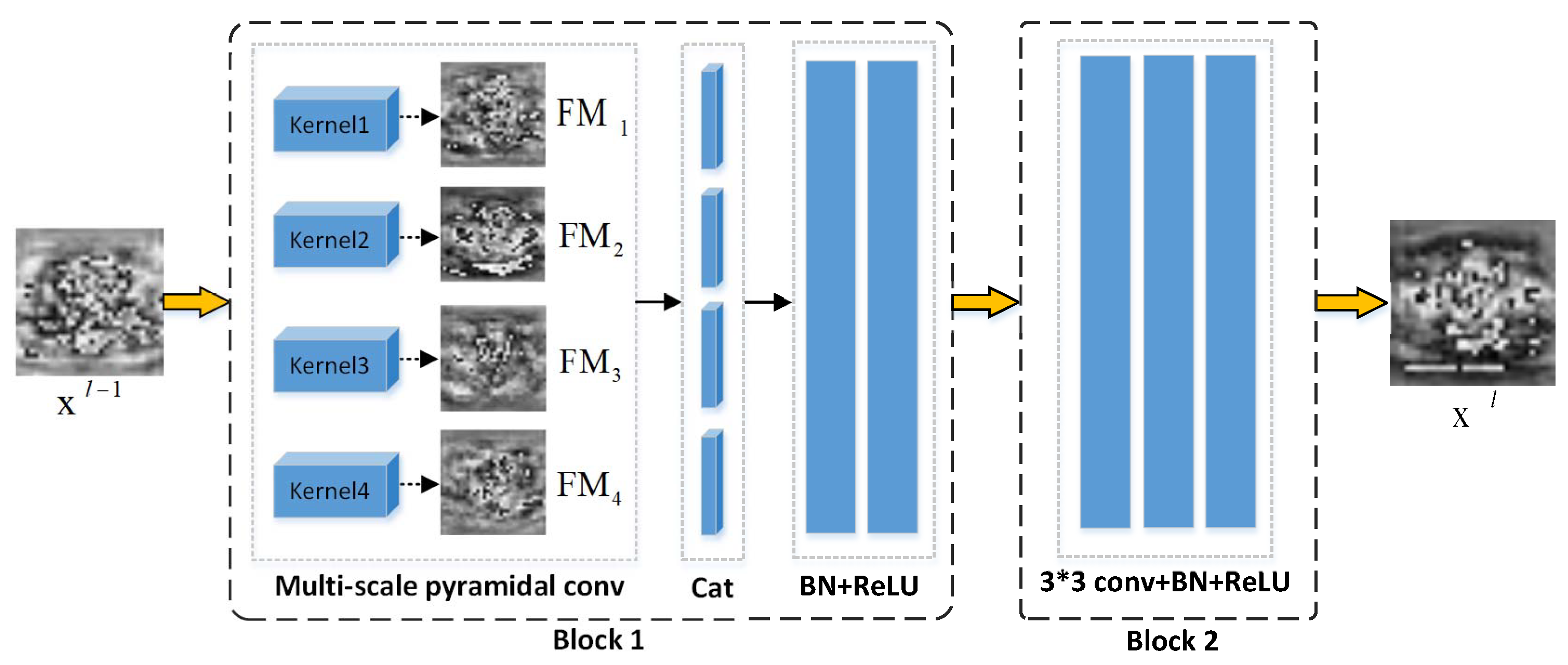
In image classification or segmentation tasks with differently shaped target regions, using the fixed kernel size convolution may neglect in part the useful detailed context and eventually lead to poor results [30]. Inspired by the literature [19], we designed a novel multi-scale pyramidal convolution (MSPC) with an encoder to tackle the problem of feature extraction due to large tumor shape variations. As shown in Figure 3, MSPC contains different levels of kernels with varying size and depth, and it can effectively capture the local contextual information in parallel.
Specifically, at layer l, given an input MRI image or a feature map , where c represents the number of image channels, h and w are the dimensions of the image. At block 1, the MSPC first utilizes different levels of kernels to generate four feature maps. All feature maps have the same dimensions and channels. Then, the feature maps are cascaded in the channel dimension, which is denoted as follows:
where represents the multi-level convolution kernels. and represent the convolution operation and offset at l layer, respectively. is the feature map generated by the kernel. is the result of the cascading multi-scale feature maps in the channel dimension. Then, the feature map is processed by batch normalization and the relu nonlinear activation function. The process can be expressed as follows:
Subsequently, we adopt the common 3 × 3 convolution with batch normalization and the relu nonlinear activation function to further enrich the extracted multi-scale features and then obtain the in block 2. After stacking a series of MSPC convolution blocks with downsampling operations to gradually encode input images, we finally obtain high-level feature representation , which is 1/16 of the input dimensions of . In this way, contains richly detailed local semantic information.
It is worth noting that the MSPC is implemented by deep separable convolution, which maintains a similar number of parameters and computation costs as traditional convolutions.
3.2. Transformer Bottleneck
In the encoder, the is obtained, but it still lacks global contextual semantic feature information. To overcome this, a transformer bottleneck is designed to learn long-range correlations with a global receptive field. As shown in Figure 2, the transformer bottleneck expects a sequence as input. Following the TransBTS [28], the high-level feature representation is arranged in a dimension sequence, where represents the size of each image patch. Then, the image patch sequences are fed into the transformer bottleneck. It is worth noting that we do not split the feature map into patches.
In the transformer bottleneck, to ensure comprehensive feature representation, a linear projection is used to map each image patch into a latent N-dimensional embedding space () and increase the nonlinearity of high-level features. Meanwhile, the position information of the sequence is crucial for the segmentation task. Hence, we introduce the learnable position-embedding function to encode the location information and directly added the feature map as follows:
where represents the linear projection, and . is the position embedding information, and denotes the feature embedding and then inputs this to the transformer layer to learn the global information representation efficiency.
As shown in Figure 4, the transformer bottleneck has L = 6 standard transformer layers. Each of them consists of a multi-head self-attention (MHSA) and a multilayer perceptron (MLP) block. Specifically, at the l layer, given the input , the self-attention of a triple is computed from the input as:
where are the learnable parameters and d is the dimensions of the triple . denotes the layer normalization. Then, the self-attention (SA) is formulated as:
MHSA is an extension with k independent SA operations and concatenates their outputs as:
where , . Finally, the output is calculated by the MLP block with residual connections as:
After all transformer layers were transformed, we obtained the , which contains different levels of coarse- and fine-grained information that is useful in recovering the image details. Notably, to input the features into the decoder, we also designed a feature mapping system that reshaped the to a standard 3D feature map where .
3.3. Decoder with Spatial Context Fusion
Effectively recovering the image details based on the semantic feature maps obtained by the encoder is very important for the decoder, which can affect the quality of the recovered images. To obtain high-quality pixel-level segmentation results in the original 2D image space, a decoder with a spatial context fusion module (SCFM) is proposed, as shown in the right part of Figure 2. The detailed structure of SCFM is shown in Figure 5. In the decoder, several cascaded upsampling convolution operations are gradually employed to restore the original image size. Moreover, additional skip connections are added to increase the spatial resolution of the semantic information.
For spatial context fusion, a spatial attention mechanism is adopted to adaptively focus on the tumor area. The spatial position weights are learned through carefully designed modules and multiplied with the input feature maps; then, the results are concatenated. Specifically, given a decoder feature map of , we use the max pooling and average pooling operations to aggregate the spatial information of and concatenate them according to the channel dimension. Then, a 3 × 3 convolution and sigmoid function are utilized to obtain the spatial weights and multiply them with . This process is shown in the following formula:
where represents the sigmoid function. is the 7 × 7 convolution. In order to transfer the weighted information to the coarse-grained feature map, a convolution is used to decrease the channel dimension and then interpolated to the same size as the input image as follows:
where represents the interpolation function. is the 1 × 1 convolution. is the weighted feature map we need. Finally, we obtained four decoder feature maps—, , and —after the skip connection structure, and we cascaded the corresponding weighted feature maps—, , and —through the channel dimension. In the last layer of the decoder, the feature maps F and are cascaded to integrate the dual branches of context and semantic information, and the pixel-level segmentation results are obtained after convolution layer processing. Meanwhile, the sigmoid function is used to compress the pixel value to range [0, 1], using 0.5 as the threshold to obtain the segmentation results of the bladder tumor foreground and background.
4. Experiments
4.1. Dataset
The dataset was acquired from the Affiliated Hospital of Shandong University of Traditional Chinese Medicine, including 86 patients, with a total of 1320 bladder cancer T2-weighted MRI images. All samples were collected using a magnetic resonance apparatus (GE Discovery MR 750). The thickness of the slices was 1 mm, and the interval between the slices was also 1 mm. The acquisition time of the 3D scans ranged from 160.456 to 165.135 s. The repetition and echo times were 2500 ms and 135 ms, respectively. The image size was uniformly set to , and each image was marked with tumor regions by experienced clinicians.
4.2. Experiments and Implementation Details
To evaluate the effectiveness of each new module in MSEDTNet, we first conducted serval ablation experiments. The differences among ablation models are listed in Table 1. We selected the vanilla UNet as the baseline model. The BaseNet, BaseMNet and BaseMTNet are new modules gradually added to the baseline model. The MSEDTNet is our proposed model.
We further compared the proposed method with existing segmentation methods (see Section 2), including Dolz et al. [16], Ge et al. [17] and Liu et al. [18]. In addition, we also compared the performance with start-of-the-art segmentation methods, such as UNet, DeepLabv3+ [31] and TransUNet [27]. However, a direct performance comparison with previous related segmentation methods has two challenges when used to perform this task. On the one hand, the relevant studies mentioned above were not able to evaluate the performance on publicly available datasets. Moreover, the source code used to replicate the work is not publicly available. On the other hand, performance evaluation metrics are not uniform for these works. Hence, for fair performance comparison, we re-trained all compared methods using our bladder cancer dataset. The other settings of the compared models are identical to those presented in the original paper.
All comparison models are implemented in the PyTorch deep learning framework [32] and ran on the machine equipped with an NVIDIA Tesla V100 GPU with 32 GB of memory. These networks are trained from scratch using an Adam optimizer with a decaying learning rate initialized at 10 . For all training cases, data augmentations, such as random rotation, flapping and shift, are used to increase data diversity. During the training process, 16 images are grouped as a mini batch. Standard five-fold cross-validation is also employed for all experiments to evaluate the robustness and generalization performance. In addition, the imbalance between foreground and background segmentation tasks may cause segmentation bias. Therefore, we used the Dice coefficient as the loss function to optimize the proposed method.
4.3. Evaluate Metrics
The Dice similarity coefficient (DSC), Jaccard index (JI) and 95th percentage of asymmetric Hausdorff Distance (95HD) were employed for the quantitative evaluation of bladder cancer segmentation. DSC and JI are sensitive to bladder cancer area, where 95HD is sensitive to tumor shape. These metrics are calculated as follows:
where X and Y are the segmentation results and ground truth, and x and y are the voxels in X and Y, respectively.
5. Results and Analysis
5.1. Ablation Study
Table 2 presents the quantitative results of ablation experiments. All metrics are represented by mean ± standard deviation. From the experimental results, it can be seen that the segmentation performance of the algorithm is improved to a certain extent after adding those modules, and MSPC is the most effective. For instance, BaseMNet achieves a JI of 80.51 and DSC of 90.45, which is 1.47% and 2.51% higher than BaseNet, respectively. This superior performance may benefit from the semantic information learned from the local multi-scale feature integration. As a basic feature extraction unit, these results also demonstrate that MSPC can effectively facilitate the identification of the various shapes of bladder cancer lesions. Other improvement strategies, which focus on modeling the high-level semantic feature information of the model, thus provide smaller enhancements to the experimental results. We use MSEDTNet as the basic comparison model in the following experiments.
We then evaluate the impact of MSPC at different scales. MSPC represents each layer of the convolution block containing the designed multi-scale pyramidal convolution in a network encoder. In MSPC, different levels of convolution kernels have a certain influence on the performance of the algorithm. To further investigate this impact, we use different levels of convolution kernels for experimental comparison and analysis. The experimental results are shown in Table 3. Intuitively, these results illustrate that in the current bladder cancer segmentation task, where the tumor has large tumor shape variations, the use of moderate perceptual fields, i.e., convolution kernels, can better extract pixel-level features from the underlying layers of the image.
Figure 6a,b reports the results of our ablation study on different numbers of transformer layers (L) in the transformer bottleneck. Testing with different layer numbers resulted in minor changes in the performance of the proposed method. These results reveal that the transformer layer has a strong ability to capture the global semantic features, but the number of transformer layers is insensitive to the effect of global information modeling. Furthermore, we further explore the various feature embedding dimensions (N) for the transformer bottleneck. As shown in Figure 6c, the model with N = 512 achieves the best score in terms of JI and DSC. We observe that increasing the number of embedding dimensions may not improve the model performance yet may result in extra computational costs. In the current task, L = 6 and N = 512 are the trade-off between performance and model complexity.
We finally evaluate the effectiveness of our proposed SCMF. By introducing the spatial context fusion module in the decoder, our segmentation model outperforms the other methods. Figure 7 provides the input image and the corresponding spatial attention map of the last SCFM layer. Intuitively, SCMF acts as a plug-in module in the decoder, allowing the decoder to focus on the tumor region by computing the spatial attention weights, which in turn improves the segmentation performance of the model. From Figure 7, we observe that SCMF can accurately concentrate on the tumor region, which is represented by the red area in the spatial attention map. It is also clear from the experimental results in Table 2 that SCMF contributes to the segmentation results. In addition, it can also be inferred from the results that MSPC and the transformer bottleneck can cope better with the deformation challenges in the tumor region.
5.2. Segmentation Results
We conducted several comparative experiments with the previous segmentation method. Table 4 reports the results on the segmentation of bladder tumors using MRI. In general, all of the methods yielded promising results, especially UNet and its improved versions, which achieved a similar performance. Among them, MSEDTNet obtained a higher accuracy than other models in almost all metrics. The mean Dice score and mean Jaccard index of MSEDTNet were 92.35 and 83.46, respectively, where the former is 4.41% higher and the latter is 4.41% higher than that of the vanilla UNet. The 95HD improved by less, relative to the other two metrics. In Table 4, we also observe that DeepLabv3+ achieves relatively poor results. The reason for this may be that the DeepLabv3+ has a strong representation capability and an over-fitting problems occur on simple medical image data. This is also the reason we chose UNet as the benchmark model for improvement.
Dilated convolution or atrous spatial pyramid pooling allow multi-scale feature extraction by increasing the receptive field of networks, and they achieve some performance gains (i.e., Ge et al. [17]). However, dilated convolution has problems with the loss of local information and the grid effect caused by the lack of correlation of information acquired at a distance, which is detrimental to fine-grained semantic segmentation [33,34]. Contrary to this, we propose multiple MSPC for parsing the feature maps provided by different levels of encoders. MSPC, by setting multiple convolution operations at different scales, can not only process the input using increasing kernel sizes in parallel and enlarge the receptive field, capturing different levels of detail, but it can also aggregate local texture information and advance the segmentation performance of the algorithm. On top of these advantages, MSPC is very efficient, and with our implementation, it can maintain similar parameters and computational costs as the conventional standard convolution.
Compared with traditional encoder–decoder architecture models, such as UNet, Table 2 and Table 4 show that the transformer architecture plays a crucial role in performance improvement. In semantic segmentation tasks, the pure transformer encoders tend to model global semantic information, usually ignoring fine-grained information at low resolution, which hampers the ability of the decoder to recover the image details [35]. Thus, the encoder with downsampling combined with transformer may be a reasonable choice, which can complement each other in coarse-grained and fine-grained information to parse the input effectively. Note that while the related TransUNet achieved closer results than MSEDTNet, our method can obtain lower parameters and reasoning time, as illustrated in Figure 8a,b.
Adding additional branches to the decoder is essential for recovering detailed image information [36,37]. For example, Liu et al. [18] produced three predicted masks from different decoders to enhance the segmentation capability, and their experiment results report a higher DSC score. Meanwhile, MSEDTNet employs five additional branches and the spatial attention mechanism to assist the decoder in resolving image details. From this perspective, SCMF also makes full use of the semantic context and high-level feature information extracted by the encoder.
We also show a visual comparison of the bladder cancer segmentation results of various methods in Figure 9. It is evident that MSEDTNet can describe bladder tumors more accurately and generate much better segmentation masks by complementing local and global semantic information, and modeling long-range dependencies. The masks predicted by other comparative models can detect inhomogeneously distributed tumor regions, but the results are also unsatisfactory for tumor boundaries with intensity inhomogeneities.
6. Conclusions
We report a newly designed framework that incorporates the multi-scale pyramidal convolution, the spatial context fusion module and the transformer bottleneck in a U-shaped network for bladder cancer segmentation. The resulting architecture, called MSEDTNet, not only has a strong ability to extract detailed local multi-scale information but also utilizes the transformer structure to capture the global semantic segmentation information of the context and fusion inherent to the multi-level feature maps of the encoder. Comprehensive experimental results show that the MSEDTNet can accommodate large tumor shape variations and has a high-performance advantage over other segmentation algorithms, therefore being expected to provide an effective segmentation tool to aid the clinical diagnosis of bladder cancer. The proposed method can be also applied to other small or variable-shape tumor segmentation tasks. In the future, we will collect more clinical data and consider including the classification and staging of bladder cancer.
Author Contributions
Investigation, X.Y.; methodology, Y.W.; writing—original draft, Y.W.; writing—review and editing, X.Y. All authors have read and agreed to the published version of the manuscript.
Funding
This research was funded by the National Natural Science Foundation of China (NSFC), grant number: 41876100.
Institutional Review Board Statement
The study was conducted in accordance with the Declaration of Helsinki and approved by the Institutional Ethics Committee of the Affiliated Hospital of Shandong University of Traditional Chinese Medicine.
Informed Consent Statement
Not applicable.
Data Availability Statement
The data presented in this study are available on request from the corresponding authors.
Conflicts of Interest
The authors declare no conflict of interest.
Abbreviations
The following abbreviations are used in this manuscript:
| MSPC | Multi-Scale Pyramidal Convolution |
| SCFM | Spatial Context Fusion Module |
| SA | Self-Attention |
| MHSA | Multi-Head Self-Attention |
| MLP | Multilayer Perceptron |
| JI | Jaccard Index |
| DSC | Dice Similarity Coefficient |
| 95HD | 95th Percentage of Asymmetric Hausdorff Distance |
References
- Barani, M.; Hosseinikhah, S.M.; Rahdar, A.; Farhoudi, L.; Arshad, R.; Cucchiarini, M.; Pandey, S. Nanotechnology in bladder cancer: Diagnosis and treatment. Cancers 2021, 13, 2214. [Google Scholar] [CrossRef]
- Antoni, S.; Ferlay, J.; Soerjomataram, I.; Znaor, A.; Jemal, A.; Bray, F. Bladder cancer incidence and mortality: A global overview and recent trends. Eur. Urol. 2017, 71, 96–108. [Google Scholar] [CrossRef] [PubMed]
- Baressi Šegota, S.; Lorencin, I.; Smolić, K.; Anḍelić, N.; Markić, D.; Mrzljak, V.; Štifanić, D.; Musulin, J.; Španjol, J.; Car, Z. Semantic Segmentation of Urinary Bladder Cancer Masses from CT Images: A Transfer Learning Approach. Biology 2021, 10, 1134. [Google Scholar] [CrossRef] [PubMed]
- Bandyk, M.G.; Gopireddy, D.R.; Lall, C.; Balaji, K.; Dolz, J. MRI and CT bladder segmentation from classical to deep learning based approaches: Current limitations and lessons. Comput. Biol. Med. 2021, 134, 104472. [Google Scholar] [CrossRef] [PubMed]
- Borhani, S.; Borhani, R.; Kajdacsy-Balla, A. Artificial intelligence: A promising frontier in bladder cancer diagnosis and outcome prediction. Crit. Rev. Oncol. 2022, 171, 103601. [Google Scholar] [CrossRef]
- Gandi, C.; Vaccarella, L.; Bientinesi, R.; Racioppi, M.; Pierconti, F.; Sacco, E. Bladder cancer in the time of machine learning: Intelligent tools for diagnosis and management. Urol. J. 2021, 88, 94–102. [Google Scholar] [CrossRef]
- Liu, H.; Zhang, Q.; Liu, Y. Image Segmentation of Bladder Cancer Based on DeepLabv3+. In Proceedings of the 2021 Chinese Intelligent Systems Conference; Springer: Berlin/Heidelberg, Germany, 2022; pp. 614–621. [Google Scholar]
- Li, L.; Liang, Z.; Wang, S.; Lu, H.; Wei, X.; Wagshul, M.; Zawin, M.; Posniak, E.J.; Lee, C.S. Segmentation of multispectral bladder MR images with inhomogeneity correction for virtual cystoscopy. In Proceedings of the Medical Imaging 2008: Physiology, Function, and Structure from Medical Images. International Society for Optics and Photonics; SPIE: Bellingham, WA, USA, 2008; Volume 6916, p. 69160U. [Google Scholar]
- Costa, M.J.; Delingette, H.; Ayache, N. Automatic segmentation of the bladder using deformable models. In Proceedings of the 2007 4th IEEE International Symposium on Biomedical Imaging: From Nano to Macro, Arlington, VA, USA, 12–15 April 2007; pp. 904–907. [Google Scholar]
- Duan, C.; Liang, Z.; Bao, S.; Zhu, H.; Wang, S.; Zhang, G.; Chen, J.J.; Lu, H. A coupled level set framework for bladder wall segmentation with application to MR cystography. IEEE Trans. Med. Imaging 2010, 29, 903–915. [Google Scholar] [CrossRef] [Green Version]
- Gsaxner, C.; Pfarrkirchner, B.; Lindner, L.; Pepe, A.; Roth, P.M.; Egger, J.; Wallner, J. PET-train: Automatic ground truth generation from PET acquisitions for urinary bladder segmentation in CT images using deep learning. In Proceedings of the 2018 11th Biomedical Engineering International Conference (BMEiCON), Chiang Mai, Thailand, 21–24 November 2018; pp. 1–5. [Google Scholar]
- Hammouda, K.; Khalifa, F.; Soliman, A.; Ghazal, M.; Abou El-Ghar, M.; Badawy, M.; Darwish, H.; Khelifi, A.; El-Baz, A. A multiparametric MRI-based CAD system for accurate diagnosis of bladder cancer staging. Comput. Med. Imaging Graph. 2021, 90, 101911. [Google Scholar] [CrossRef]
- Hu, H.; Zheng, Y.; Zhou, Q.; Xiao, J.; Chen, S.; Guan, Q. MC-Unet: Multi-scale convolution unet for bladder cancer cell segmentation in phase-contrast microscopy images. In Proceedings of the 2019 IEEE International Conference on Bioinformatics and Biomedicine (BIBM), San Diego, CA, USA, 18–21 November 2019; pp. 1197–1199. [Google Scholar]
- Liang, Y.; Zhang, Q.; Liu, Y. Automated Bladder Lesion Segmentation Based on Res-Unet. In Proceedings of the 2021 Chinese Intelligent Systems Conference; Springer: Singapore, 2022; pp. 606–613. [Google Scholar]
- Li, Z.; Feng, N.; Pu, H.; Dong, Q.; Liu, Y.; Liu, Y.; Xu, X. PIxel-Level Segmentation of Bladder Tumors on MR Images Using a Random Forest Classifier. Technol. Cancer Res. Treat. 2022, 21, 15330338221086395. [Google Scholar] [CrossRef]
- Dolz, J.; Xu, X.; Rony, J.; Yuan, J.; Liu, Y.; Granger, E.; Desrosiers, C.; Zhang, X.; Ben Ayed, I.; Lu, H. Multiregion segmentation of bladder cancer structures in MRI with progressive dilated convolutional networks. Med. Phys. 2018, 45, 5482–5493. [Google Scholar] [CrossRef]
- Ge, R.; Cai, H.; Yuan, X.; Qin, F.; Huang, Y.; Wang, P.; Lyu, L. MD-UNET: Multi-input dilated U-shape neural network for segmentation of bladder cancer. Comput. Biol. Chem. 2021, 93, 107510. [Google Scholar] [CrossRef] [PubMed]
- Liu, J.; Liu, L.; Xu, B.; Hou, X.; Liu, B.; Chen, X.; Shen, L.; Qiu, G. Bladder cancer multi-class segmentation in mri with pyramid-in-pyramid network. In Proceedings of the 2019 IEEE 16th International Symposium on Biomedical Imaging (ISBI 2019), Venice, Italy, 8–11 April 2019; pp. 28–31. [Google Scholar]
- Duta, I.C.; Liu, L.; Zhu, F.; Shao, L. Pyramidal convolution: Rethinking convolutional neural networks for visual recognition. arXiv 2020, arXiv:2006.11538. [Google Scholar]
- Li, C.; Fan, Y.; Cai, X. PyConvU-Net: A lightweight and multiscale network for biomedical image segmentation. BMC Bioinform. 2021, 22, 1–11. [Google Scholar] [CrossRef] [PubMed]
- Yu, L.; Wu, H.; Zhong, Z.; Zheng, L.; Deng, Q.; Hu, H. TWC-Net: A SAR ship detection using two-way convolution and multiscale feature mapping. Remote Sens. 2021, 13, 2558. [Google Scholar] [CrossRef]
- Zhang, N.; Zhang, Y.; Li, X.; Cong, J.; Li, X.; Wei, B. Segmentation algorithm of lightweight bladder cancer MRI images based on multi-scale feature fusion. J. Shanxi Norm. Univ. (Nat. Sci. Ed.) 2022, 50, 89–95. [Google Scholar]
- Wolf, T.; Debut, L.; Sanh, V.; Chaumond, J.; Delangue, C.; Moi, A.; Cistac, P.; Rault, T.; Louf, R.; Funtowicz, M.; et al. Transformers: State-of-the-art natural language processing. In Proceedings of the 2020 Conference on Empirical Methods in Natural Language Processing: System Demonstrations; Association for Computational Linguistics: Stroudsburg, PA, USA, 2020; pp. 38–45. [Google Scholar]
- Dosovitskiy, A.; Beyer, L.; Kolesnikov, A.; Weissenborn, D.; Zhai, X.; Unterthiner, T.; Dehghani, M.; Minderer, M.; Heigold, G.; Gelly, S.; et al. An image is worth 16x16 words: Transformers for image recognition at scale. arXiv 2020, arXiv:2010.11929. [Google Scholar]
- Zheng, S.; Lu, J.; Zhao, H.; Zhu, X.; Luo, Z.; Wang, Y.; Fu, Y.; Feng, J.; Xiang, T.; Torr, P.H.; et al. Rethinking semantic segmentation from a sequence-to-sequence perspective with transformers. In Proceedings of the IEEE/CVF Conference on Computer vision and Pattern Recognition, Nashville, TN, USA, 20–25 June 2021; pp. 6881–6890. [Google Scholar]
- Cao, H.; Wang, Y.; Chen, J.; Jiang, D.; Zhang, X.; Tian, Q.; Wang, M. Swin-unet: Unet-like pure transformer for medical image segmentation. arXiv 2021, arXiv:2105.05537. [Google Scholar]
- Chen, J.; Lu, Y.; Yu, Q.; Luo, X.; Adeli, E.; Wang, Y.; Lu, L.; Yuille, A.L.; Zhou, Y. Transunet: Transformers make strong encoders for medical image segmentation. arXiv 2021, arXiv:2102.04306. [Google Scholar]
- Wang, W.; Chen, C.; Ding, M.; Yu, H.; Zha, S.; Li, J. Transbts: Multimodal brain tumor segmentation using transformer. In Proceedings of the International Conference on Medical Image Computing and Computer-Assisted Intervention; Springer: Cham, Switzerland, 2021; pp. 109–119. [Google Scholar]
- Ronneberger, O.; Fischer, P.; Brox, T. U-net: Convolutional networks for biomedical image segmentation. In Proceedings of the International Conference on Medical Image Computing and Computer-Assisted Intervention; Springer: Cham, Switzerland, 2015; pp. 234–241. [Google Scholar]
- Liu, Y.; Li, X.; Li, T.; Li, B.; Wang, Z.; Gan, J.; Wei, B. A deep semantic segmentation correction network for multi-model tiny lesion areas detection. BMC Med. Informatics Decis. Mak. 2021, 21, 1–9. [Google Scholar] [CrossRef]
- Chen, L.C.; Zhu, Y.; Papandreou, G.; Schroff, F.; Adam, H. Encoder-decoder with atrous separable convolution for semantic image segmentation. In Proceedings of the European Conference on Computer Vision (ECCV), Munich, Germany, 8–14 September 2018; pp. 801–818. [Google Scholar]
- Paszke, A.; Gross, S.; Massa, F.; Lerer, A.; Bradbury, J.; Chanan, G.; Killeen, T.; Lin, Z.; Gimelshein, N.; Antiga, L.; et al. Pytorch: An imperative style, high-performance deep learning library. Adv. Neural Inf. Process. Syst. 2019, 32, 1–12. [Google Scholar]
- Wang, P.; Chen, P.; Yuan, Y.; Liu, D.; Huang, Z.; Hou, X.; Cottrell, G. Understanding convolution for semantic segmentation. In Proceedings of the 2018 IEEE winter conference on applications of computer vision (WACV), Lake Tahoe, NV, USA, 12–15 March 2018; pp. 1451–1460. [Google Scholar]
- Wu, T.; Tang, S.; Zhang, R.; Cao, J.; Li, J. Tree-structured kronecker convolutional network for semantic segmentation. In Proceedings of the 2019 IEEE International Conference on Multimedia and Expo (ICME), Shanghai, China, 8–12 July 2019; pp. 940–945. [Google Scholar]
- Petit, O.; Thome, N.; Rambour, C.; Themyr, L.; Collins, T.; Soler, L. U-net transformer: Self and cross attention for medical image segmentation. In Proceedings of the International Workshop on Machine Learning in Medical Imaging; Springer: Cham, Switzerland, 2021; pp. 267–276. [Google Scholar]
- Peng, C.; Ma, J. Semantic segmentation using stride spatial pyramid pooling and dual attention decoder. Pattern Recognit. 2020, 107, 107498. [Google Scholar] [CrossRef]
- Xu, R.; Wang, C.; Xu, S.; Meng, W.; Zhang, X. DC-net: Dual context network for 2D medical image segmentation. In Proceedings of the International Conference on Medical Image Computing and Computer-Assisted Intervention; Springer: Cham, Switzerland, 2021; pp. 503–513. [Google Scholar]
Figure 1.
Challenges in bladder cancer segmentation are shown by the arrows: (A) tiny tumor area, (B) intensity of inhomogeneity and weak tumor boundaries, and (C) discrete tumor distribution.
Figure 1.
Challenges in bladder cancer segmentation are shown by the arrows: (A) tiny tumor area, (B) intensity of inhomogeneity and weak tumor boundaries, and (C) discrete tumor distribution.

Figure 2.
The architecture of MSEDTNet, which is composed of an encoder, bottleneck, decoder and skip connections.
Figure 2.
The architecture of MSEDTNet, which is composed of an encoder, bottleneck, decoder and skip connections.

Figure 3.
The architecture of the proposed multi-scale encoder with MSPC and traditional convolution block.
Figure 3.
The architecture of the proposed multi-scale encoder with MSPC and traditional convolution block.

Figure 4.
The schematic of the transformer layer.

Figure 5.
The details of the spatial context fusion module.

Figure 6.
Ablation experiments with various transformer layers (a,b) and embedding dimensions (c).

Figure 7.
Visualization of the input image, mask, spatial attention map and prediction result.


Table 1.
Ablation models.
| Model | Description |
|---|---|
| BaseNet | vanilla UNet baseline |
| BaseMNet | baseline + MSPC |
| BaseMTNet | baseline + MSPC + transformer |
| MSEDTNet | baseline + MSPC + transformer + SCFM |
Table 2.
Segmentation results on different ablation models.
| Model | JI (%) ↑ | DSC (%) ↑ | 95HD (mm) ↓ |
|---|---|---|---|
| BaseNet | 79.04 ± 1.35 | 87.94 ± 0.89 | 3.96 ± 0.11 |
| BaseMNet | 80.51 ± 1.32 | 90.45 ± 1.17 | 3.97 ± 0.12 |
| BaseMTNet | 82.63 ± 1.33 | 91.16 ± 1.12 | 3.87 ± 0.10 |
| MSEDTNet | 83.46 ± 1.26 | 92.35 ± 1.19 | 3.64 ± 0.18 |
Table 3.
Segmentation results on different levels of convolution kernels.
| Kernel Size | JI (%) ↑ | DSC (%) ↑ | 95HD (mm) ↓ |
|---|---|---|---|
| 1,3,5,7 | 81.27 ± 0.98 | 90.45 ± 1.02 | 3.78 ± 0.14 |
| 1,3,9,11 | 81.32 ± 1.18 | 90.15 ± 0.86 | 3.48 ± 0.29 |
| 1,5,9,11 | 82.39 ± 1.13 | 91.32 ± 1.21 | 3.82 ± 0.22 |
| 1,7,9,11 | 83.09 ± 0.89 | 91.62 ± 1.39 | 3.61 ± 0.63 |
| 3,5,7,9 | 83.46 ± 1.26 | 92.35 ± 1.19 | 3.64 ± 0.18 |
| 3,5,7,11 | 83.44 ± 1.16 | 92.32 ± 1.26 | 3.64 ± 0.16 |
| 3,5,9,11 | 83.45 ± 0.84 | 92.12 ± 1.12 | 3.69 ± 0.19 |
| 3,7,9,11 | 83.42 ± 1.05 | 91.96 ± 1.43 | 3.78 ± 0.25 |
| 5,7,9,11 | 82.32 ± 1.42 | 90.98 ± 0.93 | 3.75 ± 0.19 |
Table 4.
Segmentation results of different methods.
| Model | JI (%) ↑ | DSC (%) ↑ | 95HD (mm) ↓ |
|---|---|---|---|
| DeepLabv3+ | 78.11 ± 1.16 | 87.38 ± 0.74 | 4.06 ± 0.12 |
| UNet | 79.04 ± 1.35 | 87.94 ± 0.89 | 3.96 ± 0.11 |
| Dolz et al. [16] | 79.51 ± 1.16 | 88.38 ± 0.74 | 3.98 ± 0.14 |
| Ge et al. [17] | 80.08 ± 1.38 | 89.43 ± 0.93 | 3.81 ± 0.23 |
| Liu et al. [18] | 79.91 ± 1.09 | 89.74 ± 1.02 | 3.84 ± 0.18 |
| TransUNet | 81.02 ± 1.36 | 90.87 ± 1.01 | 3.79 ± 0.19 |
| MSEDTNet | 83.46 ± 1.26 | 92.35 ± 1.19 | 3.64 ± 0.18 |
Publisher’s Note: MDPI stays neutral with regard to jurisdictional claims in published maps and institutional affiliations. |
© 2022 by the authors. Licensee MDPI, Basel, Switzerland. This article is an open access article distributed under the terms and conditions of the Creative Commons Attribution (CC BY) license (https://creativecommons.org/licenses/by/4.0/).
Share and Cite
MDPI and ACS Style
Wang, Y.; Ye, X. MSEDTNet: Multi-Scale Encoder and Decoder with Transformer for Bladder Tumor Segmentation. Electronics 2022, 11, 3347. https://doi.org/10.3390/electronics11203347
AMA Style
Wang Y, Ye X. MSEDTNet: Multi-Scale Encoder and Decoder with Transformer for Bladder Tumor Segmentation. Electronics. 2022; 11(20):3347. https://doi.org/10.3390/electronics11203347
Chicago/Turabian StyleWang, Yixing, and Xiufen Ye. 2022. "MSEDTNet: Multi-Scale Encoder and Decoder with Transformer for Bladder Tumor Segmentation" Electronics 11, no. 20: 3347. https://doi.org/10.3390/electronics11203347
Note that from the first issue of 2016, this journal uses article numbers instead of page numbers. See further details here.