
Power and Energy Applications Based on Quantum Computing: The Possible Potentials of Grover’s Algorithm
 , ,
, ,  and
and 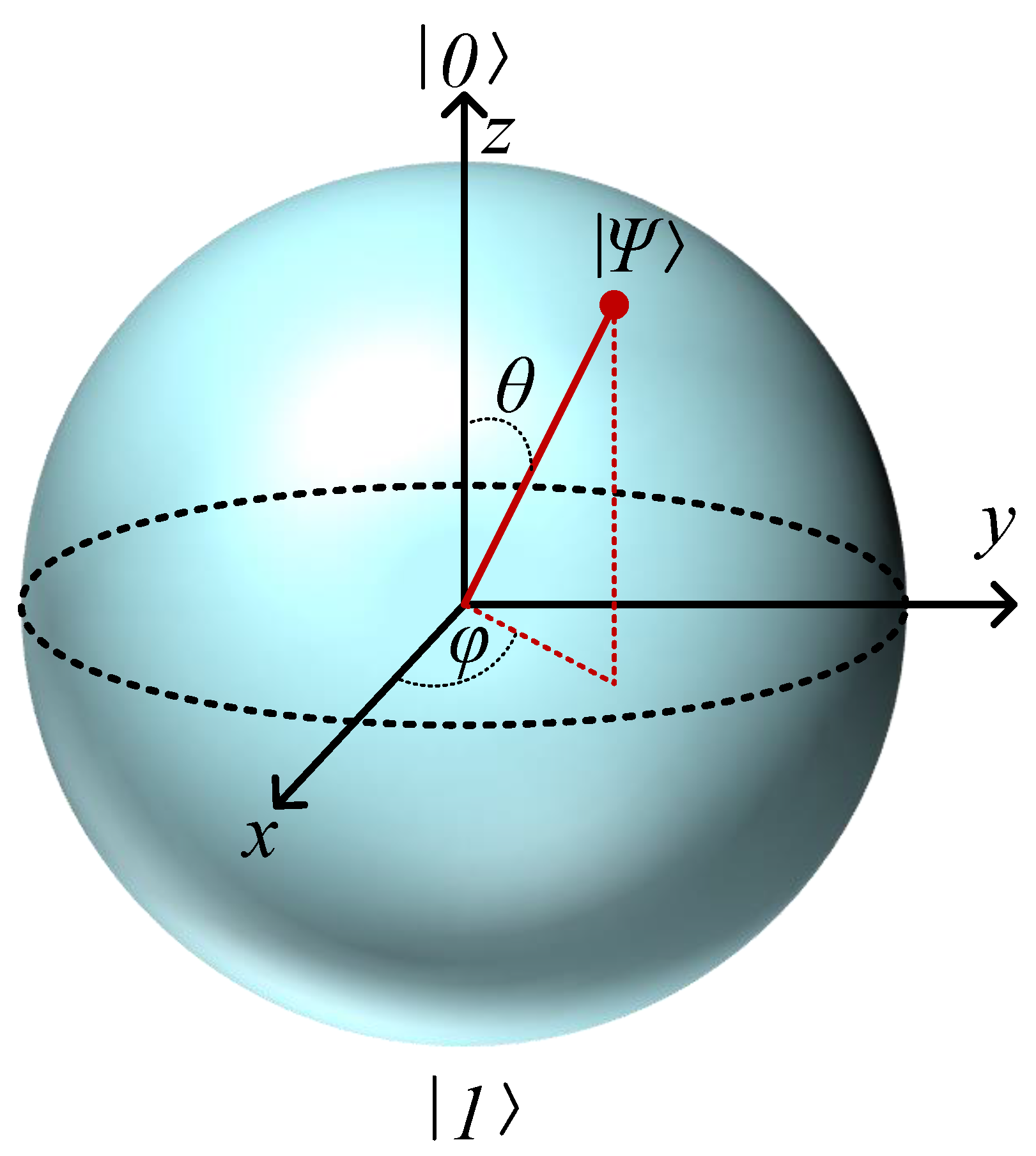
Abstract
:1. Introduction
2. Introduction to Quantum Bit
3. Basics of the Unstructured Search Problem and Grover’s Algorithm
3.1. Unstructured Search Problem
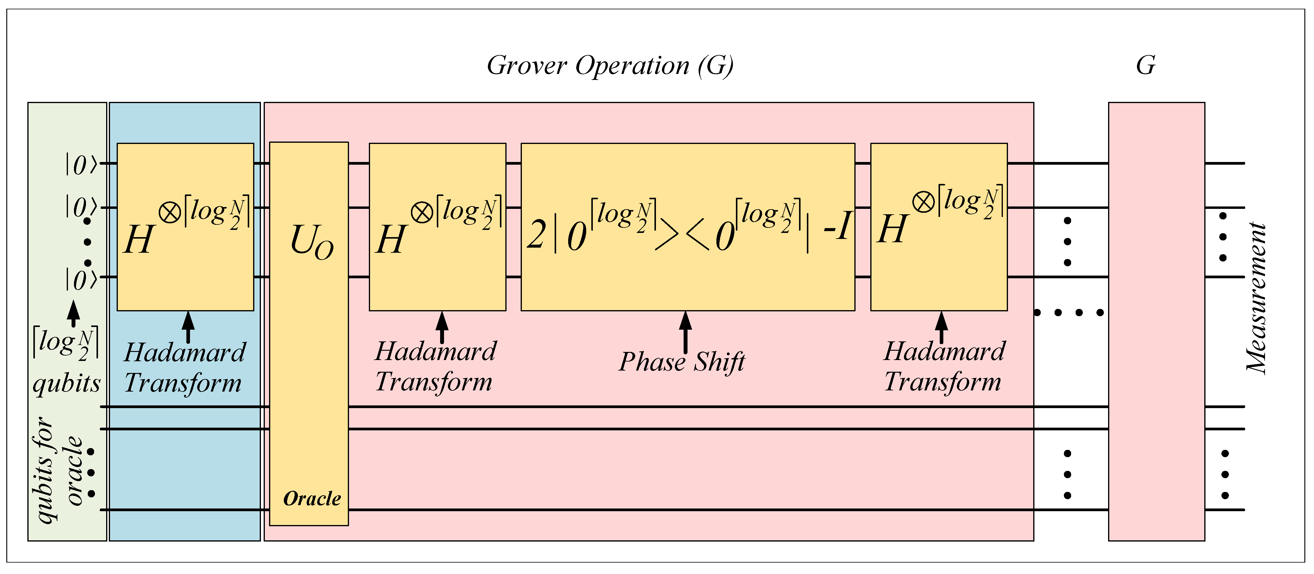
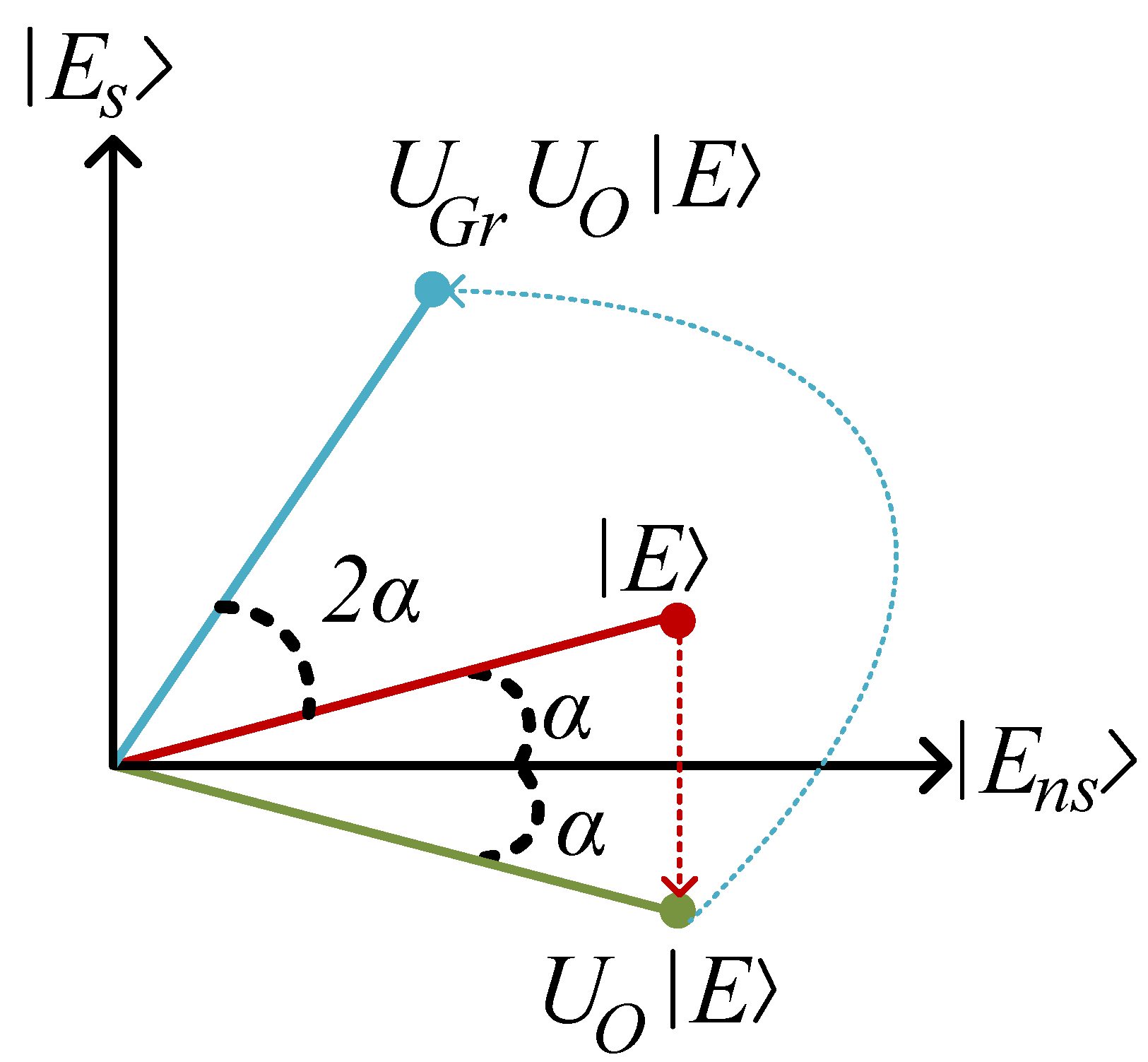
3.2. Introduction to Grover’s Algorithm
4. Potential of Grover’s Algorithm in Power and Energy Applications
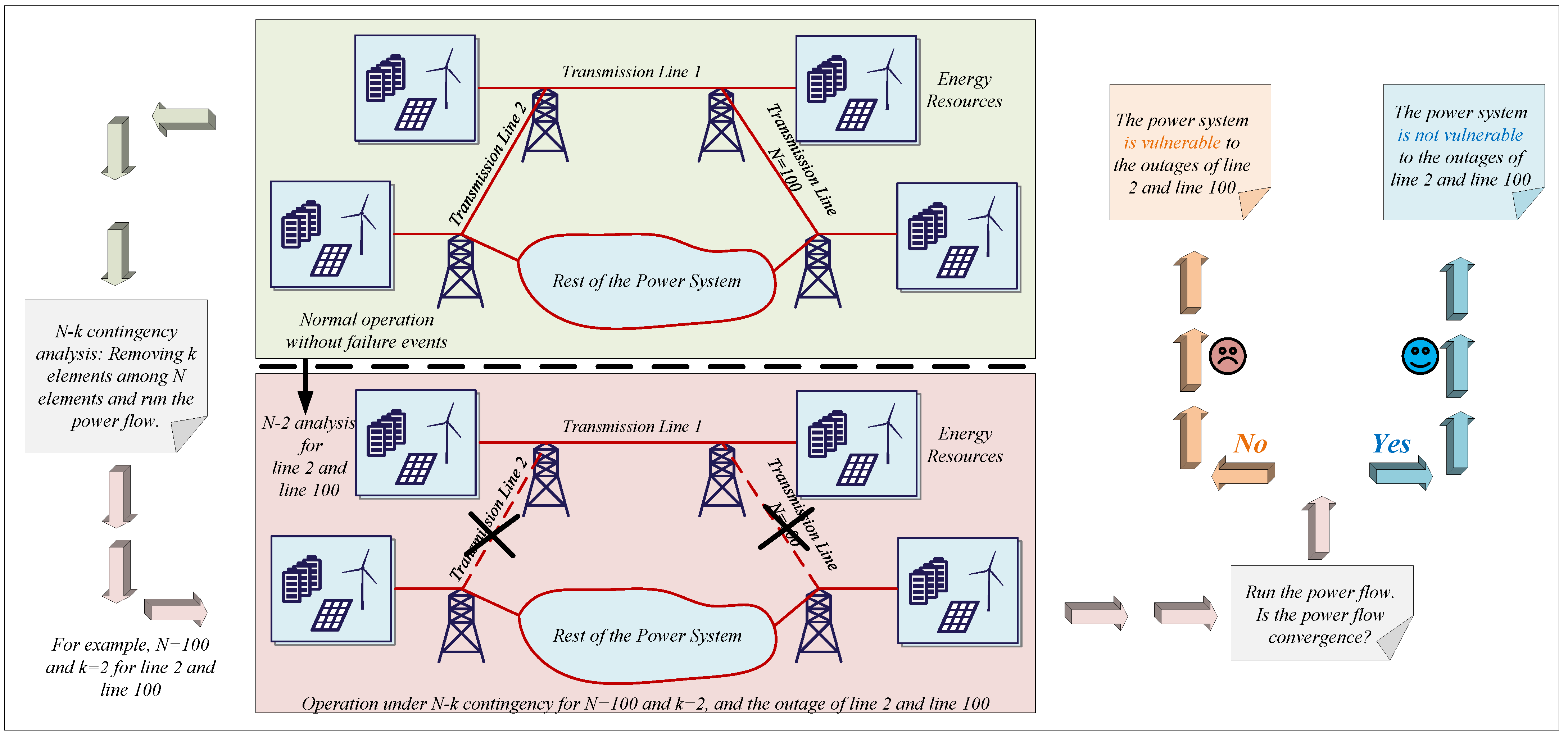
4.1. Reliability Assessment of Power Systems
4.2. Optimizations in PE Applications
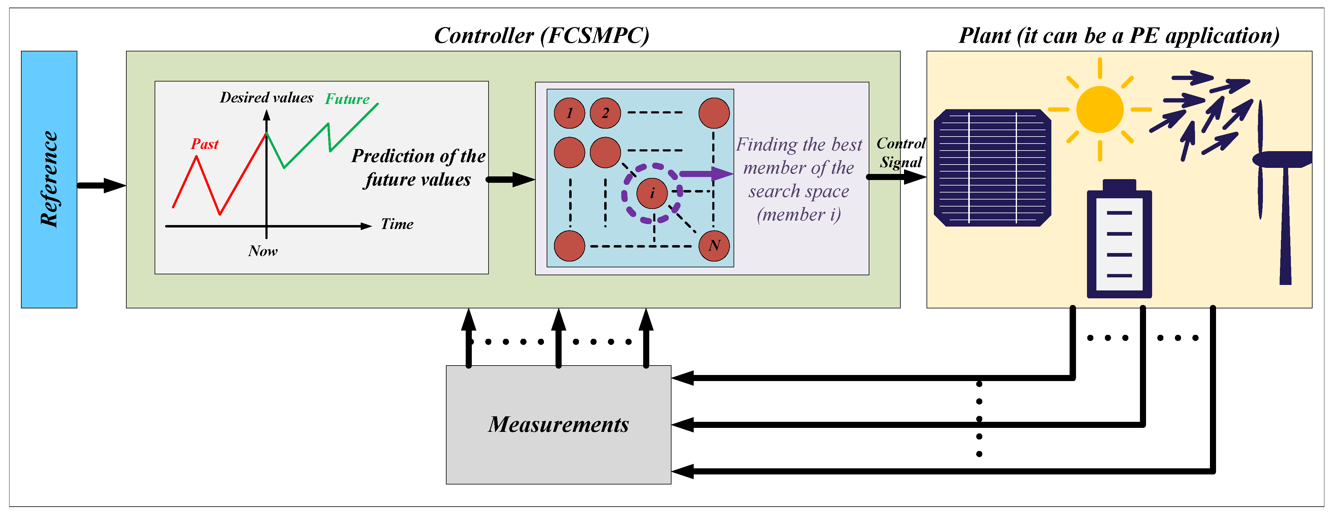
4.3. Control of PE Applications
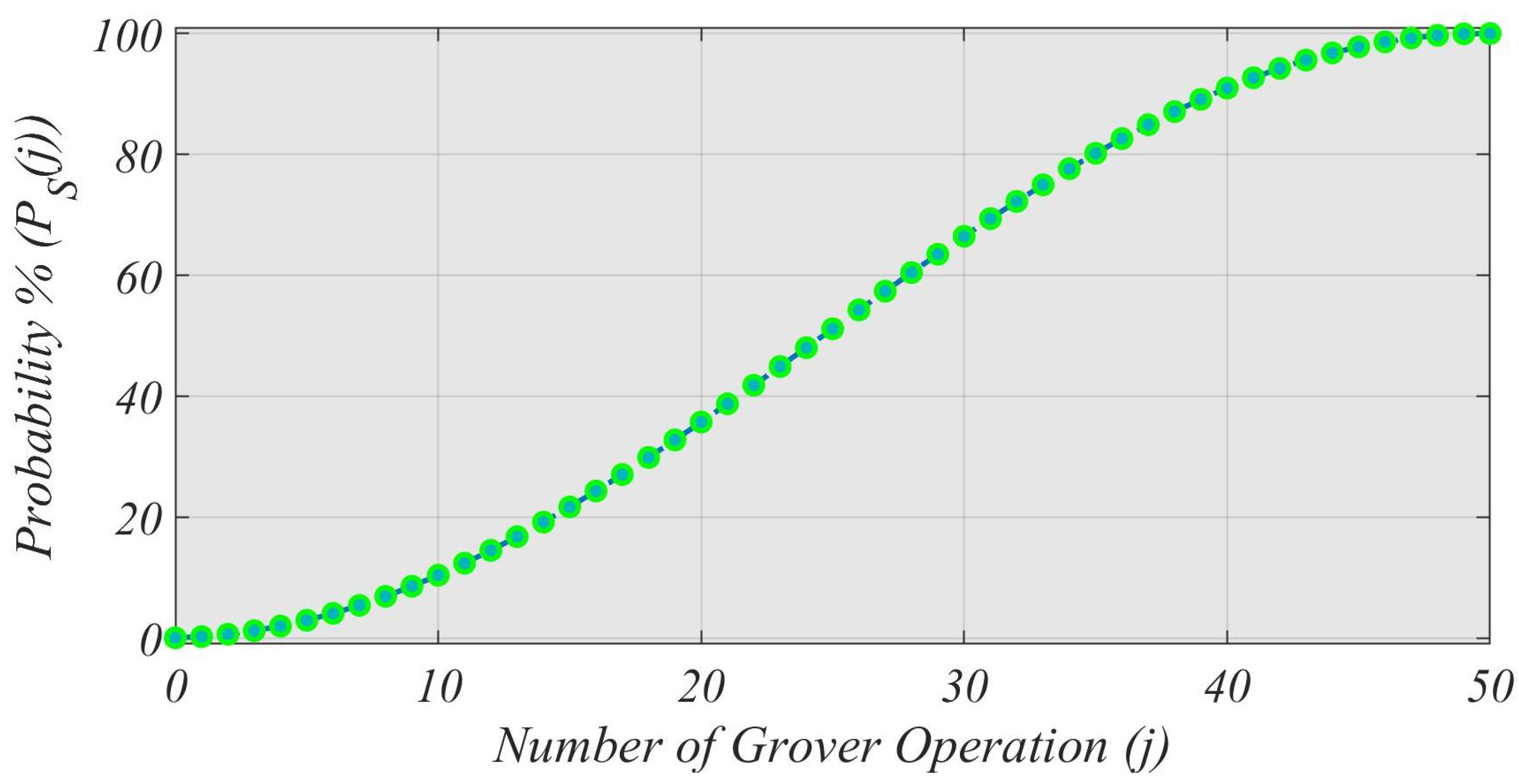
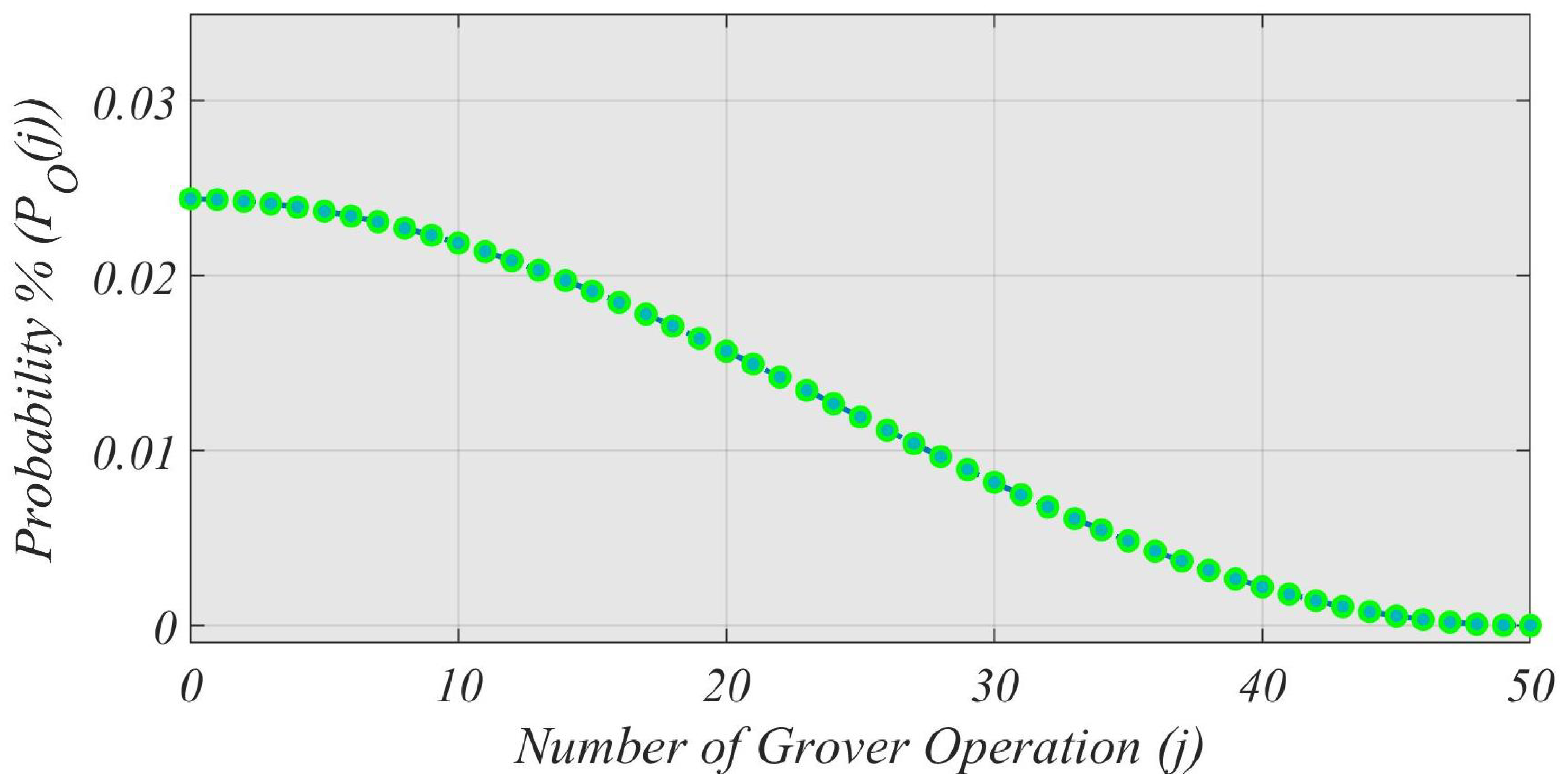
5. Example to Show the Accuracy of Grover’s Algorithm
6. Discussion
7. Conclusions and Future Directions
Author Contributions
Funding
Data Availability Statement
Conflicts of Interest
Appendix A
References
- Benioff, P. The computer as a physical system: A microscopic quantum mechanical Hamiltonian model of computers as represented by Turing machines. J. Stat. Phys. 1980, 22, 563–591. [Google Scholar] [CrossRef]
- Shor, P. Algorithms for quantum computation: Discrete logarithms and factoring. In Proceedings of the 35th Annual Symposium on Foundations of Computer Science, Santa Fe, NM, USA, 20–22 November 1994; pp. 124–134. [Google Scholar] [CrossRef]
- Grover, L.K. A Fast Quantum Mechanical Algorithm for Database Search. In Proceedings of the STOC ’96: Twenty-Eighth Annual ACM Symposium on Theory of Computing, Philadelphia, PA, USA, 22–24 May 1996; Association for Computing Machinery: New York, NY, USA, 1996; pp. 212–219. [Google Scholar] [CrossRef]
- Nielsen, M.A.; Chuang, I. Quantum Computation and Quantum Information: 10th Anniversary Edition; Cambridge University Press: Cambridge, UK, 2011. [Google Scholar]
- Zhou, Y.; Feng, F.; Zhang, P. Quantum Electromagnetic Transients Program. IEEE Trans. Power Syst. 2021, 36, 3813–3816. [Google Scholar] [CrossRef]
- Feng, F.; Zhou, Y.; Zhang, P. Quantum Power Flow. IEEE Trans. Power Syst. 2021, 36, 3810–3812. [Google Scholar] [CrossRef]
- Zhou, Y.; Zhang, P. Noise-Resilient Quantum Machine Learning for Stability Assessment of Power Systems. IEEE Trans. Power Syst. 2022. [Google Scholar] [CrossRef]
- Tang, Z.; Qin, Y.; Jiang, Z.; Krawec, W.O.; Zhang, P. Quantum-Secure Microgrid. IEEE Trans. Power Syst. 2021, 36, 1250–1263. [Google Scholar] [CrossRef]
- Yan, R.; Wang, Y.; Dai, J.; Xu, Y.; Liu, A.Q. Quantum-Key-Distribution-Based Microgrid Control for Cybersecurity Enhancement. IEEE Trans. Ind. Appl. 2022, 58, 3076–3086. [Google Scholar] [CrossRef]
- Tang, Z.; Zhang, P.; Krawec, W.O.; Jiang, Z. Programmable Quantum Networked Microgrids. IEEE Trans. Quantum Eng. 2020, 1, 1–13. [Google Scholar] [CrossRef]
- Nikmehr, N.; Zhang, P.; Bragin, M. Quantum Distributed Unit Commitment. IEEE Trans. Power Syst. 2022, 37, 3592–3603. [Google Scholar] [CrossRef]
- Feng, F.; Zhang, P.; Zhou, Y.; Tang, Z. Quantum microgrid state estimation. Electr. Power Syst. Res. 2022, 212, 108386. [Google Scholar] [CrossRef]
- Soltanmanesh, A.; Shafiee, A. Clausius inequality versus quantum coherence. Eur. Phys. J. Plus 2019, 134, 282. [Google Scholar] [CrossRef]
- Soltanmanesh, A.; Naeij, H.R.; Shafiee, A. Can thermodynamic Behavior of Alice’s Particle Affect Bob’s particle? Sci. Rep. 2020, 10, 1–12. [Google Scholar] [CrossRef] [PubMed]
- Soltanmanesh, A.; Shafiee, A. Quantum Decoherence in System-Bath Interferometry. arXiv 2018, arXiv:1802.07468. [Google Scholar]
- Vinod, G.M.; Shaji, A. Finding Solutions to the Integer Case Constraint Satisfiability Problem Using Grover’s Algorithm. IEEE Trans. Quantum Eng. 2021, 2, 1–13. [Google Scholar] [CrossRef]
- Habibi, M.R.; Baghaee, H.R.; Dragičević, T.; Blaabjerg, F. Detection of False Data Injection Cyber-Attacks in DC Microgrids Based on Recurrent Neural Networks. IEEE J. Emerg. Sel. Top. Power Electron. 2021, 9, 5294–5310. [Google Scholar] [CrossRef]
- Habibi, M.R.; Baghaee, H.R.; Blaabjerg, F.; Dragičević, T. Secure Control of DC Microgrids for Instant Detection and Mitigation of Cyber-Attacks Based on Artificial Intelligence. IEEE Syst. J. 2021, 16, 2580–2591. [Google Scholar] [CrossRef]
- Habibi, M.R.; Dragicevic, T.; Blaabjerg, F. Secure Control of DC Microgrids under Cyber-Attacks based on Recurrent Neural Networks. In Proceedings of the 2020 IEEE 11th International Symposium on Power Electronics for Distributed Generation Systems (PEDG), Dubrovnik, Croatia, 28 September–1 October 2020; pp. 517–521. [Google Scholar] [CrossRef]
- Habibi, M.R.; Baghaee, H.R.; Dragičević, T.; Blaabjerg, F. False Data Injection Cyber-Attacks Mitigation in Parallel DC/DC Converters Based on Artificial Neural Networks. IEEE Trans. Circuits Syst. II Express Briefs 2021, 68, 717–721. [Google Scholar] [CrossRef]
- Habibi, M.R.; Sahoo, S.; Rivera, S.; Dragičević, T.; Blaabjerg, F. Decentralized Coordinated Cyberattack Detection and Mitigation Strategy in DC Microgrids Based on Artificial Neural Networks. IEEE J. Emerg. Sel. Top. Power Electron. 2021, 9, 4629–4638. [Google Scholar] [CrossRef]
- Chew, B.S.H.; Xu, Y.; Wu, Q. Voltage Balancing for Bipolar DC Distribution Grids: A Power Flow Based Binary Integer Multi-Objective Optimization Approach. IEEE Trans. Power Syst. 2019, 34, 28–39. [Google Scholar] [CrossRef] [Green Version]
- Kigsirisin, S.; Miyauchi, H. Short-Term Operational Scheduling of Unit Commitment Using Binary Alternative Moth-Flame Optimization. IEEE Access 2021, 9, 12267–12281. [Google Scholar] [CrossRef]
- Montoya, O.D.; Rivas-Trujillo, E.; Hernández, J.C. A Two-Stage Approach to Locate and Size PV Sources in Distribution Networks for Annual Grid Operative Costs Minimization. Electronics 2022, 11, 961. [Google Scholar] [CrossRef]
- Kim, D.; Yoon, K.; Lee, S.H.; Park, J.W. Optimal Placement and Sizing of an Energy Storage System Using a Power Sensitivity Analysis in a Practical Stand-Alone Microgrid. Electronics 2021, 10, 1598. [Google Scholar] [CrossRef]
- Katyara, S.; Shaikh, M.F.; Shaikh, S.; Khand, Z.H.; Staszewski, L.; Bhan, V.; Majeed, A.; Shah, M.A.; Zbigniew, L. Leveraging a Genetic Algorithm for the Optimal Placement of Distributed Generation and the Need for Energy Management Strategies Using a Fuzzy Inference System. Electronics 2021, 10, 172. [Google Scholar] [CrossRef]
- Hannan, M.A.; Abdolrasol, M.G.M.; Faisal, M.; Ker, P.J.; Begum, R.A.; Hussain, A. Binary Particle Swarm Optimization for Scheduling MG Integrated Virtual Power Plant Toward Energy Saving. IEEE Access 2019, 7, 107937–107951. [Google Scholar] [CrossRef]
- Priyadarshini, S.; Kumar Panigrahi, C. Comparative Analysis between Binary Grey Wolf and Binary Bat Optimization for Optimal PMU Placement with Complete Observability. In Proceedings of the 2020 IEEE International Women in Engineering (WIE) Conference on Electrical and Computer Engineering (WIECON-ECE), Bhubaneswar, India, 26–27 December 2020; pp. 422–425. [Google Scholar] [CrossRef]
- Pedrasa, M.A.A.; Spooner, T.D.; MacGill, I.F. Scheduling of Demand Side Resources Using Binary Particle Swarm Optimization. IEEE Trans. Power Syst. 2009, 24, 1173–1181. [Google Scholar] [CrossRef]
- Adineh, B.; Habibi, M.R.; Akpolat, A.N.; Blaabjerg, F. Sensorless Voltage Estimation for Total Harmonic Distortion Calculation Using Artificial Neural Networks in Microgrids. IEEE Trans. Circuits Syst. II Express Briefs 2021, 68, 2583–2587. [Google Scholar] [CrossRef]
- Akpolat, A.N.; Habibi, M.R.; Dursun, E.; Kuzucuoğlu, A.E.; Yang, Y.; Dragičević, T.; Blaabjerg, F. Sensorless Control of DC Microgrid Based on Artificial Intelligence. IEEE Trans. Energy Convers. 2021, 36, 2319–2329. [Google Scholar] [CrossRef]
- Chen, Z.; Yu, X.; Xu, W.; Wen, G. Modeling and Control of Islanded DC Microgrid Clusters With Hierarchical Event-Triggered Consensus Algorithm. IEEE Trans. Circuits Syst. I Regul. Pap. 2021, 68, 376–386. [Google Scholar] [CrossRef]
- Shi, M.; Shahidehpour, M.; Zhou, Q.; Chen, X.; Wen, J. Optimal Consensus-Based Event-Triggered Control Strategy for Resilient DC Microgrids. IEEE Trans. Power Syst. 2021, 36, 1807–1818. [Google Scholar] [CrossRef]
- Wang, B.; Wang, Y.; Xu, Y.; Zhang, X.; Gooi, H.B.; Ukil, A.; Tan, X. Consensus-Based Control of Hybrid Energy Storage System With a Cascaded Multiport Converter in DC Microgrids. IEEE Trans. Sustain. Energy 2020, 11, 2356–2366. [Google Scholar] [CrossRef]
- Fan, B.; Guo, S.; Peng, J.; Yang, Q.; Liu, W.; Liu, L. A Consensus-Based Algorithm for Power Sharing and Voltage Regulation in DC Microgrids. IEEE Trans. Ind. Inform. 2020, 16, 3987–3996. [Google Scholar] [CrossRef]
- Cucuzzella, M.; Trip, S.; De Persis, C.; Cheng, X.; Ferrara, A.; van der Schaft, A. A Robust Consensus Algorithm for Current Sharing and Voltage Regulation in DC Microgrids. IEEE Trans. Control. Syst. Technol. 2019, 27, 1583–1595. [Google Scholar] [CrossRef]
- Du, Y.; Lu, X.; Tang, W. Accurate Distributed Secondary Control for DC Microgrids Considering Communication Delays: A Surplus Consensus-Based Approach. IEEE Trans. Smart Grid 2022, 13, 1709–1719. [Google Scholar] [CrossRef]
- Chen, J.; Xu, C.; Wu, C.; Xu, W. Adaptive Fuzzy Logic Control of Fuel-Cell-Battery Hybrid Systems for Electric Vehicles. IEEE Trans. Ind. Inform. 2018, 14, 292–300. [Google Scholar] [CrossRef]
- Gaburro Bacheti, G.; Sartório Camargo, R.; Silva Amorim, T.; Yahyaoui, I.; Frizera Encarnação, L. Model-Based Predictive Control with Graph Theory Approach Applied to Multilevel Back-to-Back Cascaded H-Bridge Converters. Electronics 2022, 11, 1711. [Google Scholar] [CrossRef]
- Guennouni, N.; Chebak, A.; Machkour, N. Optimal Dual Active Bridge DC-DC Converter Operation with Minimal Reactive Power for Battery Electric Vehicles Using Model Predictive Control. Electronics 2022, 11, 1621. [Google Scholar] [CrossRef]
- Alidrissi, Y.; Ouladsine, R.; Elmouatamid, A.; Errouissi, R.; Bakhouya, M. Constant Power Load Stabilization in DC Microgrids Using Continuous-Time Model Predictive Control. Electronics 2022, 11, 1481. [Google Scholar] [CrossRef]
- Kibalama, D.; Liu, Y.; Stockar, S.; Canova, M. Model Predictive Control for Automotive Climate Control Systems via Value Function Approximation. IEEE Control Syst. Lett. 2022, 6, 1820–1825. [Google Scholar] [CrossRef]
- Sun, J.; Qiu, L.; Liu, X.; Zhang, J.; Ma, J.; Fang, Y. Improved Model Predictive Control for Three-Phase Dual-Active-Bridge Converters With a Hybrid Modulation. IEEE Trans. Power Electron. 2022, 37, 4050–4064. [Google Scholar] [CrossRef]
- Yang, Q.; Karamanakos, P.; Tian, W.; Gao, X.; Li, X.; Geyer, T.; Kennel, R. Computationally Efficient Fixed Switching Frequency Direct Model Predictive Control. IEEE Trans. Power Electron. 2022, 37, 2761–2777. [Google Scholar] [CrossRef]
- He, J.; Shi, C.; Wei, T.; Jia, D. Stochastic Model Predictive Control of Hybrid Energy Storage for Improving AGC Performance of Thermal Generators. IEEE Trans. Smart Grid 2022, 13, 393–405. [Google Scholar] [CrossRef]
- Habibi, M.R.; Baghaee, H.R.; Blaabjerg, F.; Dragicevic, T. Secure MPC/ANN-Based False Data Injection Cyber-Attack Detection and Mitigation in DC Microgrids. IEEE Syst. J. 2021, 16, 1487–1498. [Google Scholar] [CrossRef]
- Akpolat, A.N.; Habibi, M.R.; Baghaee, H.R.; Dursun, E.; Kuzucuoglu, A.E.E.; Yang, Y.; Dragicevic, T.; Blaabjerg, F. Dynamic Stabilization of DC Microgrids using ANN-Based Model Predictive Control. IEEE Trans. Energy Convers. 2021, 37, 999–1010. [Google Scholar] [CrossRef]
- Xu, W.; Elmorshedy, M.F.; Liu, Y.; Islam, M.R.; Allam, S.M. Finite-Set Model Predictive Control Based Thrust Maximization of Linear Induction Motors Used in Linear Metros. IEEE Trans. Veh. Technol. 2019, 68, 5443–5458. [Google Scholar] [CrossRef]
- Jin, T.; Shen, X.; Su, T.; Flesch, R.C.C. Model Predictive Voltage Control Based on Finite Control Set With Computation Time Delay Compensation for PV Systems. IEEE Trans. Energy Convers. 2019, 34, 330–338. [Google Scholar] [CrossRef]
- Jama, M.; Mon, B.F.; Wahyudie, A.; Mekhilef, S. Maximum Energy Capturing Approach for Heaving Wave Energy Converters Using an Estimator-Based Finite Control Set Model Predictive Control. IEEE Access 2021, 9, 67648–67659. [Google Scholar] [CrossRef]
- Falkowski, P.; Sikorski, A. Finite Control Set Model Predictive Control for Grid-Connected AC–DC Converters With LCL Filter. IEEE Trans. Ind. Electron. 2018, 65, 2844–2852. [Google Scholar] [CrossRef]
- Elmorshedy, M.F.; Xu, W.; Allam, S.M.; Rodriguez, J.; Garcia, C. MTPA-Based Finite-Set Model Predictive Control Without Weighting Factors for Linear Induction Machine. IEEE Trans. Ind. Electron. 2021, 68, 2034–2047. [Google Scholar] [CrossRef]


Publisher’s Note: MDPI stays neutral with regard to jurisdictional claims in published maps and institutional affiliations. |
© 2022 by the authors. Licensee MDPI, Basel, Switzerland. This article is an open access article distributed under the terms and conditions of the Creative Commons Attribution (CC BY) license (https://creativecommons.org/licenses/by/4.0/).
Share and Cite
Habibi, M.R.; Golestan, S.; Soltanmanesh, A.; Guerrero, J.M.; Vasquez, J.C. Power and Energy Applications Based on Quantum Computing: The Possible Potentials of Grover’s Algorithm. Electronics 2022, 11, 2919. https://doi.org/10.3390/electronics11182919
Habibi MR, Golestan S, Soltanmanesh A, Guerrero JM, Vasquez JC. Power and Energy Applications Based on Quantum Computing: The Possible Potentials of Grover’s Algorithm. Electronics. 2022; 11(18):2919. https://doi.org/10.3390/electronics11182919
Chicago/Turabian StyleHabibi, Mohammad Reza, Saeed Golestan, Ali Soltanmanesh, Josep M. Guerrero, and Juan C. Vasquez. 2022. "Power and Energy Applications Based on Quantum Computing: The Possible Potentials of Grover’s Algorithm" Electronics 11, no. 18: 2919. https://doi.org/10.3390/electronics11182919