Combining Event-Based Maneuver Selection and MPC Based Trajectory Generation in Autonomous Driving

Abstract

Maneuver planning, which plays a key role in selecting desired lanes and speeds, is an essential element of autonomous driving. Generally, for a vehicle driving on a multilane road, there are several potential maneuvers in both longitudinal and lateral directions. Selecting the best maneuver from the various options represents a significant challenge. In this paper, we propose a maneuver selection algorithm and combine it with a trajectory generation algorithm, which is based on model predictive control (MPC). The maneuver selection method is a higher-level planner, which selects only one maneuver from all possible maneuvers based on the current situation and delivers it to a lower-level MPC-based trajectory tracking controller. The effectiveness of the proposed algorithm is validated by simulating an overtaking scenario on a multilane highway.

1. Introduction

Planning appropriate maneuvers and tracking reference trajectories are fundamental tasks for an autonomous vehicle and thus must be incorporated in a control framework for autonomous vehicles. With regard to motion planning and control, there are many technical terms in the literature, including maneuver planning, task planning, motion planning, trajectory planning, and path planning [1,2,3,4,5,6,7]. There are no universal definitions for these terms, but they can usually be understood in their particular contexts.

In this paper, a maneuver (e.g., lane changing and decelerating) results from a higher-level plan. Our approach selects the maneuver that the controlled vehicle will execute at the next time step, and the selected maneuver is input to the lower-level trajectory tracking controller.

Trajectory planning techniques for autonomous vehicles can be broadly classified into four groups [4]: sampling based planning [8,9], interpolating curve planning [10,11,12,13,14], graph search-based planning [3,15,16,17], and numerical optimization [18,19,20,21].

Sampling-based planning algorithms [8,9,22] plan trajectories by randomly sampling the configuration space and finding connections [4]. These methods can provide fast solutions and have therefore been used in self-driving vehicles [22,23,24]. However, the trajectories are not continuous and therefore are uncomfortable for passengers. Interpolating curve planning methods, e.g., using Clothoid curves, polynomial curves, Bézier curves, or Spline curves [10,11,12,13,14], delivers smoother paths [4]. These methods are, e.g., used in autonomous driving when comfort and safety are major concerns and the driving environment is structured and modeled [4]. However, in general, it is difficult to obtain a global model of the environment. Graph search-based planning methods, e.g., applying Dijkstra’s algorithm [15,16], the A* algorithm [3,17], or the D* algorithm [4], determine a path from one point to another. However, these methods are not suitable for real-time applications, where dynamic obstacles present one major challenge.

Numerical optimizations [18,19,20,21] obtain the optimal trajectory by solving a constrained optimization problem. These methods can deal with constraints and uncertainties, so the controlled vehicle can take other traffic participants’ behaviors into consideration by setting appropriate collision avoidance constraints [4]. Additional advantages for applications in autonomous driving are that they can improve comfort by setting constraints on control inputs, such that the global road information is not needed when combined with a receding horizon strategy, as, e.g., in MPC, and these methods are applicable in real time and can avoid moving obstacles. However, the computational complexity of MPC poses a challenge because the optimization of the cost functions needs to be performed at every time step for a potentially long prediction horizon [18].

MPC attracted attention in autonomous driving because of its ability to deal with constraints caused by traffic rules, physical limitations, and collision avoidance. It predicts future driving behavior based on vehicle models, including the point-mass model, the kinematic bicycle model, or the dynamic bicycle model [25]. Trajectory planning methods based on MPC have been proposed, e.g., in [18,26,27,28]. In [18], multiple feasible maneuvers are obtained using the maneuver planning method and these maneuvers are delivered to the lower-level MPC controller for trajectory control. However, delivering multiple maneuvers to the lower-level MPC might cause unnecessary computational burden. This has motivated us to identify a better maneuver selection method, which finally selects only one maneuver from all feasible/possible maneuvers, and then delivers this maneuver to the lower-level MPC controller.

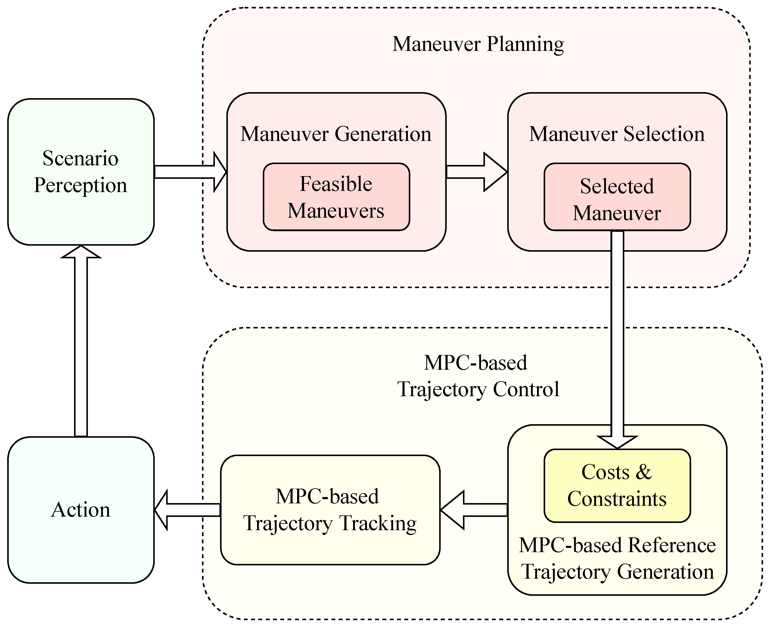
We propose a high-level maneuver planning method and combine it with a low-level MPC-based trajectory control. The framework used in this paper, shown in Figure 1, consists of four main modules: scenario perception, maneuver planning, MPC-based trajectory control, and action. Our main concerns here are maneuver planning and MPC-based trajectory control. The maneuver planning module contains two consecutive submodules: maneuver generation and maneuver selection. Similarly, the MPC-based trajectory control consists of two submodules: MPC-based reference trajectory generation and MPC-based trajectory tracking.

Our method is based upon the method presented in [6]. We utilize the maneuver generation method from [6] and improve it to make it more applicable in reality by removing the necessity to explore an exceeding number of trajectories. Then we employ an MPC controller instead of the sliding mode controller for tracking to avoid high switching frequencies and to be able to take into account constraints.

Our maneuver planning and trajectory control method works as follows: at each time step, (1) we generate all possible maneuvers employing the maneuver generation method from [6]; then, (2) select the desired lane and the longitudinal speed maneuver using a maneuver selection method; after that, the trajectory control module (3) generates a reference trajectory based on the selected maneuver, and (4) tracks it. More specifically, a group of candidate maneuvers is initially generated with respect to the environment in which the method in [6] is employed. Next, maneuvers which contribute less to meeting the criteria for the best maneuver are excluded from these candidate maneuvers. The criteria for excluding maneuvers involve the goal lane, the roadside edges, the time to collision (TTC) [6,29], and the intervehicular time (TIV) [6]. In the trajectory control module, the desired reference trajectory is generated by adjusting the cost function and constraints in the MPC controller to account for the selected maneuver. The reference trajectory is then tracked by MPC which, in addition, ensures that no constraints are violated.

The rest of the paper is organized as follows. Section 2 introduces the maneuver planning method, including maneuver generation and maneuver selection. In Section 3, we explain how model predictive control is applied by introducing the optimization problem of the MPC controller, a model of the vehicle, the cost function, constraints, and the trajectory generation for maneuvers. Simulation results are presented in Section 4, and Section 5 summarizes the paper and provides prospects for future research.

2. Maneuver Planning

In autonomous driving, maneuvers are the high-level strategies that describe what the vehicle will do in the short term or long term. For example, lane changing is a short-term goal and overtaking is a long-term goal. In this paper, the maneuver planning method is executed at each time step. This maneuver planning method determines what the controlled vehicle will do in the next time step, and we assume that the controlled vehicle knows the long-term goal. Our method is designed for scenarios consisting of two vehicles, where the controlled vehicle is the ego vehicle (EV), and the other one is the object vehicle (OV). The EV assumes that the OV will maintain its current velocity at each time step. In this paper, we make the common assumption that the position and velocity of the OV can be observed by the EV [30,31,32].

Maneuver planning consists of maneuver generation and maneuver selection (see Figure 1). For the maneuver generation, we use an approach presented in [6] and add a novel approach for maneuver selection that first selects only one maneuver from the generated options and then provides the maneuver information to the lower-level controller. In [6], the lower-lever controller is a second-order sliding-mode controller. Ideal sliding modes require high switching frequencies, which can burden the actuators and cause rapid wear, and, therefore, lead to safety issues. We propose to replace the sliding-mode controller with MPC to combine trajectory generation and tracking. This might again improve safety in addition to safe maneuver selection by enforcing that no safety constraints are violated.

The main task of the maneuver selection submodule is to select the appropriate lane in the lateral direction and the speed strategy in the longitudinal direction, see Section 2.3. Additionally, the safety criteria used in selecting longitudinal maneuvers are presented in Section 2.2.

2.1. Maneuver Generation

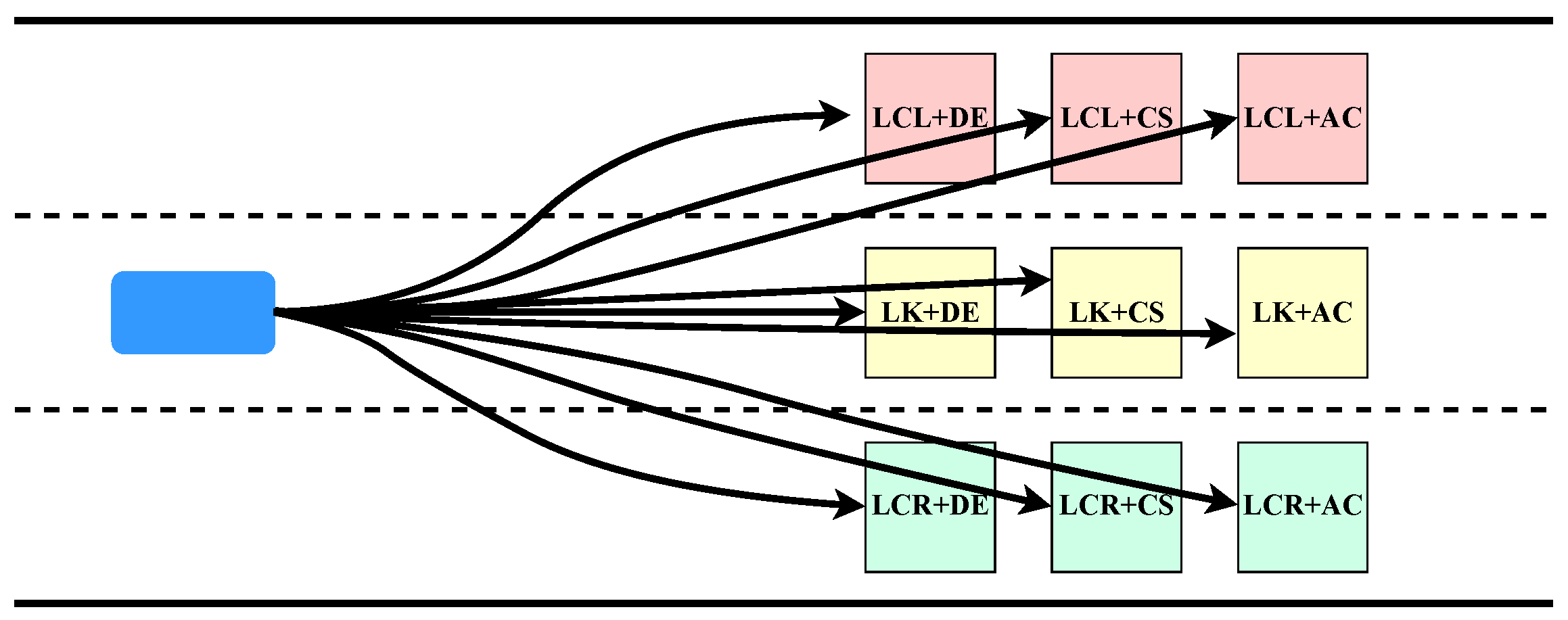
In [6], a vehicle driving on a multilane road is considered. Before a trajectory is generated, nine feasible maneuvers are generated by a combination of both lateral and longitudinal directions. In more detail, three feasible maneuvers can be chosen in the longitudinal direction: decelerating (DE), maintaining current speed (CS), accelerating (AC); meanwhile, there are three possible maneuvers in the lateral direction: changing to the left lane (LCL), staying in the current lane (LK), or changing to the right lane (LCR). Combining the maneuvers in both directions, nine combined maneuvers [6] can be obtained, as shown in Figure 2.

High-level maneuvers are then delivered to the lower-level controller for trajectory tracking. If the maneuver planning method delivers multiple feasible maneuvers to the controller, the controller will have to experience superfluous computational burden. Additionally, it is even worse when the controller is computationally expensive, for instance, MPC. Autonomous vehicles can benefit from the ability of MPC to deal with constraints. However, in order to efficiently use MPC as a low-level controller, we have to reduce the computational burden. Our maneuver selection method contributes to this by selecting only one maneuver during maneuver planning and, therefore, delivering only one maneuver to the lower-level MPC controller, as shown in Section 2.3.

2.2. Safety Criteria

When selecting one maneuver from all feasible ones, safety is one of our major concerns in both longitudinal and lateral directions. The safety criteria we use in selecting the maneuver in the longitudinal direction are the time to collision (TTC) and the intervehicular time (TIV). The risk of collision is higher for (1) high speed differences and (2) low intervehicle distances [6]. TTC [6,29] and TIV [6] can be used to quantify this risk.

TTC was first proposed by Hayward in [29] to measure the risk level of the two-vehicle scenarios where the two cars are close to each other and have different velocities. TTC can deal with both lane-keeping scenarios and lane-changing scenarios [29]. However, there exists a dangerous situation that cannot be detected by TTC: when two vehicles, at the same speed, are close to each other. In this situation, the TTC is not small, even though the two vehicles have a high likelihood of colliding. In order to also take this situation into consideration, the intervehicular time (TIV) is introduced [6].

2.2.1. TTC

In [29], Hayward gives the definition of TTC: TTC represents the time required for two vehicles to collide if they maintain their current longitudinal velocities. TTC is formulated as follows:

$$\mathrm{TTC}=\frac{\left|\Delta x_{\mathrm{ev},\mathrm{ov}}\right|}{\left|\Delta v_{\mathrm{ev},\mathrm{ov}}\right|}$$

(1)

where $\Delta x_{\mathrm{ev},\mathrm{ov}}$ is the relative distance between the EV and the OV in the longitudinal direction with $\Delta x_{\mathrm{ev},\mathrm{ov}}=x_{\mathrm{ev}}-x_{\mathrm{ov}}$, where $x_{\mathrm{ev}}$ and $x_{\mathrm{ov}}$ represent the longitudinal positions of the EV and OV, respectively. We denote the relative velocity between these two vehicles in the longitudinal direction with $\Delta v_{\mathrm{ev},\mathrm{ov}}=v_{\mathrm{ev}}-v_{\mathrm{ov}}$, where $v_{\mathrm{ev}}$ and $v_{\mathrm{ov}}$ are the longitudinal velocities of the EV and OV, respectively.

In general, a great TTC stands for a safer situation. In [6], if the TTC is greater than 10 s, it is supposed that there is no interaction between two vehicles. If the TTC is smaller than 1.5 s, the situation is considered risky and a warning system is triggered.

2.2.2. TIV

The TIV [6] can deal with the risky situation that TTC fails to detect: two vehicles with the same (or similar) high speed are close to each other in the same lane. In this situation, the TTC can be great because of the relative velocity between the two vehicles is zero (or very small). However, this is actually a risky situation, because once the leading vehicle decelerates or the following vehicle accelerates, they will most probably collide. The TIV is defined as follows:

$$\mathrm{TIV}=\frac{\left|\Delta x_{\mathrm{ev},\mathrm{ov}}\right|}{v^{*}}$$

(2)

where $\Delta x_{\mathrm{ev},\mathrm{ov}}$ is the same as that in TTC, and $v^{*}$ is the velocity of the vehicle which is following the other vehicle in the longitudinal direction. Here, $v^{*}=v_{\mathrm{ev}}$ if the EV is behind the OV, and $v^{*}=v_{\mathrm{ov}}$ if the EV is in front of the OV.

Great TIV indicates safer situations. According to [6], a TIV of 2 s is commonly used as a boundary for safety.

Great TTC and TIV indicate a lower risk level [6]. In this paper, a situation with great TTC and TIV at the same time is considered safe. Additionally, TTC and TIV might consider the following safe situation dangerous: two vehicles without the intention of changing lanes are driving in different lanes, but close to each other in the longitudinal direction. However, this false danger can be recognized with further knowledge of the lateral positions of the vehicles.

In the maneuver selection, the aim of the selection of the longitudinal maneuver is to choose a maneuver with low risk, so the maneuver which can lead to greater TTC and TIV will be selected.

2.3. Maneuver Selection

The maneuver selection method selects only one maneuver from all possible maneuvers obtained from the maneuver generation method in [6]. The main idea of our maneuver selection method is: remove less appropriate maneuvers from all possible ones obtained from the maneuver generation based on selection criteria (details will be shown later); therefore, only one maneuver is kept at the end of the maneuver selection.

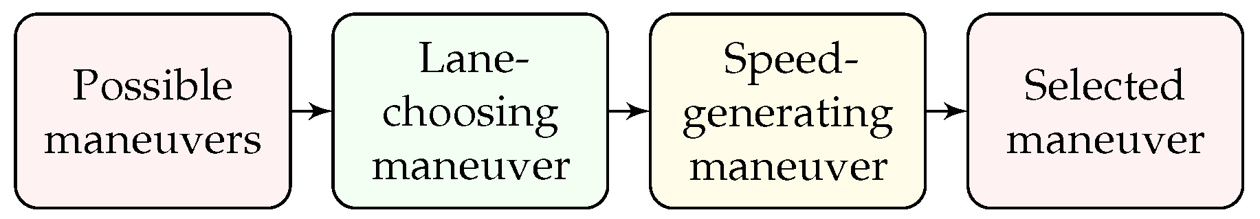
Our maneuver selection method has two tasks: (i) selecting a lane choosing maneuver in the lateral direction and (ii) obtaining a speed generating maneuver in the longitudinal direction. The maneuver selection method is shown in Figure 3, where the tasks (i) and (ii) are colored green and yellow, respectively. These two tasks in the maneuver selection method will be explained in detail below.

2.3.1. Lane-Choosing Maneuver in the Lateral Direction

In the lane-choosing maneuver in the lateral direction, we remove the less appropriate maneuvers based on the constraints from the road edges and the current goal lane of the vehicle. The process is shown as follows:

• Remove the lateral maneuvers that will cause the road edge constraints to be violated. For instance, if the vehicle is in the rightmost lane of the road, the maneuver of changing to the right lane (LCR) is inadmissible.
• Exclude the lateral maneuvers with which the vehicle is not heading towards the goal lane. Here, we consider two cases: (a) the goal lane is the current lane; (b) the goal lane is a different lane. In case (a), we simply remove the lane-changing maneuvers, LCL and LCR. Case (b) is more complicated. If the goal lane is the lane at the left (right) side of the current lane, we first exclude the lateral maneuver with which the vehicle turns to the opposite/wrong direction, LCR (LCL) is therefore removed. Then, we consider whether the lane-changing maneuver is satisfied or not. If the conditions for changing lanes are satisfied, we exclude the LK maneuver; otherwise the lane-changing maneuver LCL (LCR) is removed.

After the lane-choosing maneuver, only one maneuver in the lateral direction remains. Thus, before the only longitudinal maneuver has been selected from all three possible ones, there are three combined maneuvers left.

2.3.2. Speed Generating Maneuver in the Longitudinal Direction

To select the longitudinal maneuver, the criteria used to remove the less appropriate maneuvers from all possible maneuvers are safety, efficiency, and smoothness. Among them, safety is our prime concern. If after all less safe maneuvers have been removed, there is more than one speed maneuver left, we take into account the efficiency and smoothness to, finally, retain just one maneuver.

The safety criteria we use are TTC and TIV. Great TTC and TIV correspond to safer situations. Therefore, maneuvers that contribute to increasing TTC and TIV are kept in the selection process. The process of using TTC and TIV as criteria to select the longitudinal maneuver/maneuvers is shown in

Table 1. Selection of longitudinal maneuver based on the safety criteria TTC and TIV.

$\mathbf{\Delta }{\mathit{x}}_{\mathbf{ev},\mathbf{ov}}$	$\mathbf{\Delta }{\mathit{v}}_{\mathbf{ev},\mathbf{ov}}$	Possible Maneuver	$\left|\mathbf{\Delta }{\mathit{x}}_{\mathbf{ev},\mathbf{ov}}\right|$	$\left|\mathbf{\Delta }{\mathit{v}}_{\mathbf{ev},\mathbf{ov}}\right|$	${\mathit{v}}^{*}$	TTC	TIV	Result
		DE	↑	↑	↓	?	↑
	$\Delta v_{\mathrm{ev},\mathrm{ov}}<0$	CS	↑	−	−	↑	↑	CS
		AC	↑	↓	↑	↑	↓
		DE	↓	↓	↓	?	?
$\Delta x_{\mathrm{ev},\mathrm{ov}}<0$	$\Delta v_{\mathrm{ev},\mathrm{ov}}>0$	CS	↓	−	−	↓	↓	DE
		AC	↓	↑	↑	↓	↓
		DE	↑	↑	↓	/	↑
	$\Delta v_{\mathrm{ev},\mathrm{ov}}=0$	CS	−	−	−	/	−	DE
		AC	↓	↑	↑	/	↓
		DE	↓	↑	−	↓	↓
	$\Delta v_{\mathrm{ev},\mathrm{ov}}<0$	CS	↓	−	−	↓	↓	AC
		AC	↓	↓	−	?	↓
		DE	↑	↓	−	↑	↑
$\Delta x_{\mathrm{ev},\mathrm{ov}}>0$	$\Delta v_{\mathrm{ev},\mathrm{ov}}>0$	CS	↑	−	−	↑	↑	DE/CS
		AC	↑	↑	−	?	↑
		DE	↓	↑	−	/	↓
	$\Delta v_{\mathrm{ev},\mathrm{ov}}=0$	CS	−	−	−	/	−	AC
		AC	↑	↑	−	/	↑

.

In Table 1, the first two columns show the current relative position and velocity of the two vehicles. The third column enumerates the possible maneuvers obtained from maneuver generation. The fourth, fifth, and sixth columns demonstrate how $\left|\Delta x_{\mathrm{ev},\mathrm{ov}}\right|$, $\left|\Delta v_{\mathrm{ev},\mathrm{ov}}\right|$ and $v^{*}$ will change if the specific maneuver has been executed. The seventh and eighth columns show the trends of TTC and TIV, respectively, with the change of the $\left|\Delta x_{\mathrm{ev},\mathrm{ov}}\right|$, $\left|\Delta v_{\mathrm{ev},\mathrm{ov}}\right|$ and $v^{*}$. The last column shows the longitudinal maneuver/maneuvers left after removing maneuvers based on TTC and TIV.

We use labels ( ‘↑’, ‘↓’, ‘−’, ‘?’, and ‘/’) to briefly represent the trend of the change in the case of a specific maneuver. ‘↑’ means the value of corresponding item will increase; ‘↓’ means it is decreasing; ‘−’ means that there will be no change in terms of the corresponding value; ‘?’ means the future change is unknown; ‘/’ shows that we do not calculate the TTC when $\Delta v_{\mathrm{ev},\mathrm{ov}}=0$.

In the following, we will discuss how to choose the longitudinal maneuver in two distinct situations according to the relative positions of the two vehicles in the longitudinal direction: the EV is behind the OV, and the EV is in front of the OV.

• The EV is behind the OV; $\Delta x_{\mathrm{ev},\mathrm{ov}}<0$.
  • $\Delta v_{\mathrm{ev},\mathrm{ov}}<0$. The velocity of the EV is smaller than that of the OV:

    -

    When the EV maintains current longitudinal speed (CS), the distance between the two vehicles increases. Thus, both TTC and TIV increase as time goes on;

    -

    The EV’s choice of deceleration (DE) will cause the distance between the two vehicles ($\left|\Delta x_{\mathrm{ev},\mathrm{ov}}\right|$) to increase, but also cause the relative velocity ($\left|\Delta v_{\mathrm{ev},\mathrm{ov}}\right|$) to increase. Thus, the effect of deceleration (DE) on TTC is unknown;

    -

    Choosing acceleration (AC) will cause the TIV to decrease. Thus, we will not keep the AC.

    Therefore, maintaining current longitudinal speed (CS) is the best choice.
  • $\Delta v_{\mathrm{ev},\mathrm{ov}}>0$. The velocity of the EV is greater than that of the OV, which is dangerous:

    -

    Both maintaining current speed (CS) and acceleration (AC) will definitely cause a decrease of the TTC and TIV;

    -

    However, by executing deceleration (DE), TTC and TIV will probably trend upward.

    Consequently, deceleration (DE) is selected as the longitudinal maneuver performed in this situation.
  • $\Delta v_{\mathrm{ev},\mathrm{ov}}=0$. The two vehicles have the same longitudinal speed:

    -

    Under this circumstance, only TIV is used to estimate the risk;

    -

    Whether the distance between the two vehicles is small or not, decreasing the speed of the EV is a safe maneuver, which contributes to obtaining a greater TIV.

    Thus, deceleration (DE) is selected for the EV in this situation.
• The EV is in front of the OV; $\Delta x_{\mathrm{ev},\mathrm{ov}}>0$.
  • $\Delta v_{\mathrm{ev},\mathrm{ov}}<0$. The velocity of the EV is less than that of the OV:

    -

    Not only deceleration (DE), but also maintaining current speed (CS) will cause a decreasing trend of the TTC and TIV;

    -

    Additionally, when choosing acceleration (AC), TIV will experience a rapid drop, while TTC might show an upward trend.

    This is not a safe situation, but increasing the speed of the EV will probably contribute to avoiding possible collisions, so AC is taken as the longitudinal maneuver.
  • $\Delta v_{\mathrm{ev},\mathrm{ov}}>0$. The velocity of the EV is greater than that of the OV:

    -

    Both decelerating (DE) and maintaining current speed (CS) are beneficial to increasing TTC and TIV, so they can be taken as candidate maneuvers;

    -

    Furthermore, DE has a negative effect on the efficiency and smoothness.

    Therefore, we finally keep CS as the longitudinal maneuver in this situation.
  • $\Delta v_{\mathrm{ev},\mathrm{ov}}=0$. The EV and OV drive at same speed:

    -

    In this situation, TTC is not calculated and only TIV is considered as a safety criterion;

    -

    Increasing the speed (AC) will help obtain greater TIV;

    -

    Neither decreasing (DE), nor maintaining current speed (CS) will contribute to increasing TIV.

    Therefore, acceleration (AC) is selected.

All the situations we discuss require that the OV be within the detectable area of the EV. This is also mathematically described as $\left|\Delta x_{\mathrm{ev},\mathrm{ov}}\right|\le \Delta x^{\max }$, where $\Delta x^{\max }$ is the longitudinally maximum detectable distance.

After excluding less appropriate maneuvers in both lateral and longitudinal directions, only one longitudinal maneuver and one lateral maneuver are left. Combining the selected maneuvers in both directions, we eventually obtain a single maneuver.

3. Model Predictive Control

The maneuver selected by the maneuver selection method is delivered to the lower-level MPC-based trajectory control module, which contains two submodules, reference trajectory generation and trajectory tracking, as shown in Figure 1.

MPC is used to generate and track trajectories because it will not only consider a cost function, thus allowing for energy efficiency, but also take into account collision avoidance constraints and thus further contribute to safety. As a low-level trajectory tracking controller, MPC realizes the maneuver selected from high-level maneuver planning by setting reference states in the cost function and by adjusting constraints.

Reference trajectory generation is the first step in the MPC-based trajectory control module. However, maneuver planning and trajectory planning are coupled by specifying parameters in the cost function and in the constraints of MPC, so we will define a model, a cost function, and constraints for MPC before we introduce the trajectory generation.

3.1. Optimization Problem of the MPC Controller

At each time step, MPC minimizes an optimal control cost function with respect to constraints on a short prediction horizon to obtain the current control input. A dynamic system model is used to predict states in the prediction horizon for different choices of control input trajectories which finally allows to obtain the optimal inputs.

The constrained optimization problem that MPC solves at each time step is shown as follows:

$$\underset{u}{min}V(\xi ,u)=\underset{u}{min}\sum _{k=0}^{N-1}l(\xi \left(k\right),u\left(k\right))+V_f\left(\xi \left(N\right)\right)$$

(3a)

subject to

$$\xi (k+1)=f\left(\xi \right(k),u(k\left)\right)$$

(3b)

$$\xi \left(0\right)={\xi }_0$$

(3c)

$$\xi \left(k\right)\in \mathcal{X},k=0,\dots ,N-1$$

(3d)

$$\xi \left(N\right)\in {\mathcal{X}}_f$$

(3e)

$$u\left(k\right)\in \mathcal{U},k=0,\dots ,N-1$$

(3f)

where Equation (3a) represents the cost function. The cost function is the sum of stage costs and terminal cost for a prediction horizon of length N [33]. In Equation (3a), $V(\xi ,u)$ is the cost function, $l\left(\xi \right(k),u(k\left)\right)$ is the stage cost at time k, and $V_f\left(\xi \left(N\right)\right)$ is the terminal cost. $\xi \left(k\right)$ and $u\left(k\right)$ are the state vector and control input vector, respectively.

The constraints for states and inputs are given in Equation (3b–f). Among these, Equation (3b) is the dynamic system model, which is a vehicle model in this paper. ${\xi }_0$ is the initial state. $\mathcal{X}$, ${\mathcal{X}}_f$ and $\mathcal{U}$ are the sets of admissible states, terminal states and inputs, respectively.

We will discuss the system model, constraints, and the cost function for autonomous driving in the following subsections.

3.2. Vehicle Model

A vehicle model can be used to predict future states. Various vehicle models, with different modeling depths, e.g., point-mass model, Fiala tire model, dynamic bicycle model, or kinematic bicycle model are available [34,35,36,37,38]. In this paper, for simplicity, we choose the point-mass model [34], but any other model that includes position and speed of the vehicle is also suitable.

This point-mass model is described by the following equation

$$\xi \left(k+1\right)=A\xi \left(k\right)+Bu\left(k\right)$$

(4)

$$A=\left[\begin{array}{cccc}1& 0& T& 0\\ 0& 1& 0& T\\ 0& 0& 1& 0\\ 0& 0& 0& 1\end{array}\right],B=\left[\begin{array}{cc}{T}^2/2& 0\\ 0& T^2/2\\ T& 0\\ 0& T\end{array}\right]$$

(5)

where $\xi \left(k\right)={\left[x\left(k\right),y\left(k\right),v_x\left(k\right),v_y\left(k\right)\right]}^T$ is the state vector. $x\left(k\right)$ and $y\left(k\right)$ represent the longitudinal and lateral positions, respectively. $v_x\left(k\right)$ and $v_y\left(k\right)$ are the longitudinal and lateral velocities, respectively. $u\left(k\right)={\left[a_x\left(k\right),a_y\left(k\right)\right]}^T$ is the input vector. $a_x\left(k\right)$, $a_y\left(k\right)$ is the longitudinal and lateral acceleration, respectively. Moreover, A and B are system matrices and T is the sampling interval.

3.3. Constraints

The constraints are used to enforce restrictions on states and inputs. For our autonomous driving application, we include constraints for traffic rules, collision avoidance, and physical limitations of vehicles.

3.3.1. State Constraints

This part contains the states’ constraints for obeying traffic rules and avoiding collisions.

• Constraints for Traffic Rules:

  $$x\left(k\right)\in [0,+\infty ]$$

  (6)

  $$y\left(k\right)\in [w_{\mathrm{veh}}/2,m{w}_{\mathrm{lane}}-w_{\mathrm{veh}}/2]$$

  (7)

  $$v_x\left(k\right)\in [v_{x_{\min }},v_{x_{\max }}]$$

  (8)

  $$v_y\left(k\right)\in [v_{y_{\min }},v_{y_{\max }}]$$

  (9)

  where $w_{\mathrm{veh}}$ is the width of vehicles, $w_{\mathrm{lane}}$ is the width of each lane, and m is the number of lanes. As shown in Equation (6), the vehicle can move forward freely in the longitudinal direction. Equation (7) is designed for keeping the vehicle within the road edges. Constraints (8) and (9) give the upper and lower limits to velocities in longitudinal and lateral directions, respectively.
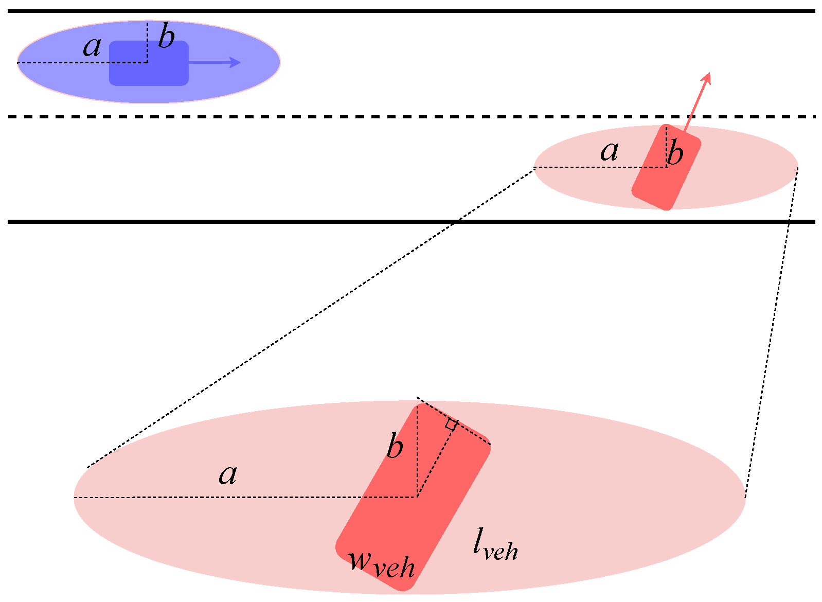
• Safety constraint:
  In order to avoid collisions, a region around each vehicle is defined that other vehicles are not allowed to enter [34,38]. The region can be any convex shape larger than the shape of the vehicle [38]. As in [34,39,40,41], an elliptic region is chosen for our implementation, as shown in Figure 4.
  This safety constraint is then realized by the following inequality:

  $$\frac{\Delta x_{\mathrm{ev},\mathrm{ov}}^2}{a^2}+\frac{\Delta y_{\mathrm{ev},\mathrm{ov}}^2}{b^2}>1,$$

  (10)

  where a and b are the major and minor axes of the ellipse, respectively. The longitudinal distance between the EV and one OV is $\Delta x_{\mathrm{ev},\mathrm{ov}}$. The lateral distance between these two vehicles is $\Delta y_{\mathrm{ev},\mathrm{ov}}$. The center of the ellipse-shaped region is the same as the center of the vehicle. Since we use a point-mass model that does not provide information about the current orientation of the vehicle, the major axis of the ellipse is chosen to be aligned with the lanes.
  For safety, the ellipse-shaped region has to be large enough that the vehicle shape is covered by the ellipse for all possible vehicle orientations. In order to find appropriate a and b, we consider the vehicle turning left or right, see Figure 4. If the vehicle is covered by the ellipse here, it will also be covered for all other orientations. Let $l_{\mathrm{veh}}$ and $w_{\mathrm{veh}}$ denote the length and the width of a vehicle, respectively. Then it holds for a and b:

  $$0<\sqrt{{\left(\frac{l_{\mathrm{veh}}}{2}\right)}^2+{\left(\frac{w_{\mathrm{veh}}}{2}\right)}^2}+\delta <b<a$$

  (11)

  where $\delta >0$.

3.3.2. Input Constraints

Input constraints are restrictions on the accelerations in both longitudinal and lateral directions. These constraints stem from the physical limitations of the vehicles.

$$a_x\left(k\right)\in [a_{{\mathrm{x}}_{\min }},a_{{\mathrm{x}}_{\max }}]$$

(12)

$$a_y\left(k\right)\in [a_{{\mathrm{y}}_{\min }},a_{{\mathrm{y}}_{\max }}]$$

(13)

3.4. Cost Function

The cost function for an MPC-controlled vehicle is designed for tracking the reference trajectory while realizing smooth and energy efficient driving.

The cost function $V(\xi ,u)$ at each time step is

$$\begin{array}{cc}\hfill V(\xi ,u)& =\sum _{k=0}^{N-1}\left[u{\left(k\right)}^{T}Qu\left(k\right)+\Delta \xi {\left(k\right)}^{T}R\Delta \xi \left(k\right)\right]\hfill \\ \hfill & +\Delta \xi {\left(N\right)}^{T}S\Delta \xi \left(N\right)\hfill \end{array}$$

(14)

where $\Delta \xi \left(k\right)=\xi \left(k\right)-{\xi }_{\mathrm{ref}}\left(k\right)$ and $\Delta \xi \left(N\right)=\xi \left(N\right)-{\xi }_{\mathrm{ref}}\left(N\right)$. ${\xi }_{\mathrm{ref}}\left(k\right)$ and ${\xi }_{\mathrm{ref}}\left(N\right)$ are the reference states for the vehicle to track. $\Delta \xi$ is the error between the predicted states and the reference states. The weighting matrices Q, R, and S are defined by $Q=\mathrm{diag}(q_1,q_2)$, $R=\mathrm{diag}(r_1,r_2,r_3,r_4)$, and $S=\mathrm{diag}(s_1,s_2,s_3,s_4)$, where $q_1$, $q_2$, $r_1$, $r_2$, $r_3$, $r_4$, $s_1$, $s_2$, $s_3$, and $s_4$ are elements in the matrices, and non-negative real numbers.

The terms $\Delta \xi {\left(k\right)}^{T}R\Delta \xi \left(k\right)$ and $\Delta \xi {\left(N\right)}^{T}S\Delta \xi \left(N\right)$ are used for tracking reference states, where, in particular, the reference lateral position and longitudinal velocity are relevant. The term $u{\left(k\right)}^{T}Qu\left(k\right)$ is designed to punish large control inputs, to ensure that the vehicle drives smoothly and in an energy-efficient way.

The cost function acts as a bridge in our combined maneuver planning and trajectory control method. The maneuver selected from the maneuver planning method determines the reference trajectories in the cost function. The reference trajectories will be tracked by minimizing the cost function with all constraints being satisfied simultaneously. In the following subsection, we will introduce the reference trajectory generation and trajectory tracking.

3.5. MPC-Based Reference Trajectory Generation

MPC-based reference trajectory generation aims to translate the selected semantic maneuver to a reference trajectory. At each time step, the selected maneuver is executed by setting appropriate costs and constraints of the MPC controller, as shown in Figure 1.

We set values of the reference states ${\xi }_{\mathrm{ref}}\left(k\right)$ and ${\xi }_{\mathrm{ref}}\left(N\right)$ in the cost function (14) based on the selected maneuver. In the reference states ${\xi }_{\mathrm{ref}}\left(k\right)={\left[x_{\mathrm{ref}}\left(k\right),y_{\mathrm{ref}}\left(k\right),v_{x,\mathrm{ref}}\left(k\right),v_{y,\mathrm{ref}}\left(k\right)\right]}^T$, the first two elements $x_{\mathrm{ref}}\left(k\right)$ and $y_{\mathrm{ref}}\left(k\right)$ are reference positions in longitudinal and lateral directions, respectively. Corresponding reference velocities are represented by $v_{x,\mathrm{ref}}\left(k\right)$ and $v_{y,\mathrm{ref}}\left(k\right)$. Among these reference states, only $y_{\mathrm{ref}}\left(k\right)$ and $v_{x,\mathrm{ref}}\left(k\right)$ are directly determined by the selected maneuver. The maneuver planning has no impact on the reference states $x_{\mathrm{ref}}\left(k\right)$ and $v_{y,\mathrm{ref}}\left(k\right)$. However, this does not mean that the maneuver planning will not affect the longitudinal position $x\left(k\right)$ and lateral velocity $v\left(k\right)$. It will affect them implicitly by the coupling of states and control inputs in the constrained optimal control problem.

The elements in the weighting matrices $R=\mathrm{diag}(r_1,r_2,r_3,r_4)$ and $S=\mathrm{diag}(s_1,s_2,s_3,s_4)$ in the cost function (14) allow tracking performances to be tuned. The maneuver planning will directly set the lateral reference position and the longitudinal reference velocity of the vehicle. Therefore, we choose $r_2,r_3,s_2,s_3>0$ and small constants are assigned to the elements $r_1,r_4,s_1$, and $s_4$.

The selected lane maneuver will determine the value of the lateral reference position $y_{\mathrm{ref}}$, and the speed maneuver will determine the longitudinal reference velocity $v_{x,\mathrm{ref}}$. $y_{\mathrm{ref}}$ is set to be the lateral center of the target lane. This applies to both lane keeping (LK) and lane changing (LCL and LCR). The rules for setting $v_{x,\mathrm{ref}}$ vary according to the relative position of the two vehicles in the lateral direction. For the situation where two vehicles are in the same lane: (1) If the selected maneuver is maintaining the current speed (CS), let $v_{x,\mathrm{ref}}$ be the same as its current longitudinal velocity; (2) For decelerating (DE), the reference velocity $v_{x,\mathrm{ref}}$ is the minimum between $75\%$ of the current longitudinal velocity of the EV and the longitudinal velocity of the vehicle in front of the EV; (3) If the vehicle intends to accelerate (AC), we specify $v_{x,\mathrm{ref}}$ to be the maximum of $125\%$ of the current longitudinal velocity of the EV, the longitudinal velocity of the OV, and the longitudinal speed limit. When the two vehicles are in the same lane, $v_{x,\mathrm{ref}}$ is equal to the speed limit.

4. Simulation Results

To validate the effectiveness of the proposed method, a simulation is conducted in MATLAB for a highway environment. In this section, we will first introduce two scenarios. Then, we explain how the maneuver planning and trajectory control method is applied. Finally, we show simulation results and discuss the effectiveness of our method.

4.1. Scenario Description

We consider two scenarios, a vehicle-following scenario and an overtaking scenario. We discuss maneuver and trajectory planning for both scenarios. However, we simulate only the overtaking scenario because it includes all lateral and longitudinal maneuvers, and car-following will occur when overtaking.

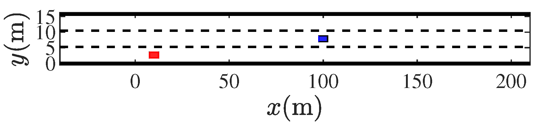
The environment is a three-lane highway. All these three lanes have the same width and there is no curvature. There are two vehicles, an EV (red) and an OV (blue), as shown in Figure 5. The three lanes are labeled as $L_0$, $L_1$, and $L_2$, respectively. The rightmost lane $L_0$ is the slow lane. The leftmost lane $L_2$ is the fast lane, which is intended to be only for overtaking. Initially, we assume that the EV is driving in the slow lane $L_0$, with longitudinal velocity 35 m/s. The OV is driving in the middle lane $L_1$ with a lower longitudinal velocity of 20 m/s. The initial longitudinal positions of EV and OV are 10 m and 90 m, respectively. On a highway, overtaking on the right side is forbidden [2]. Therefore, with these initial settings, the EV has two possible options: following the OV in $L_0$ or overtaking on the left.

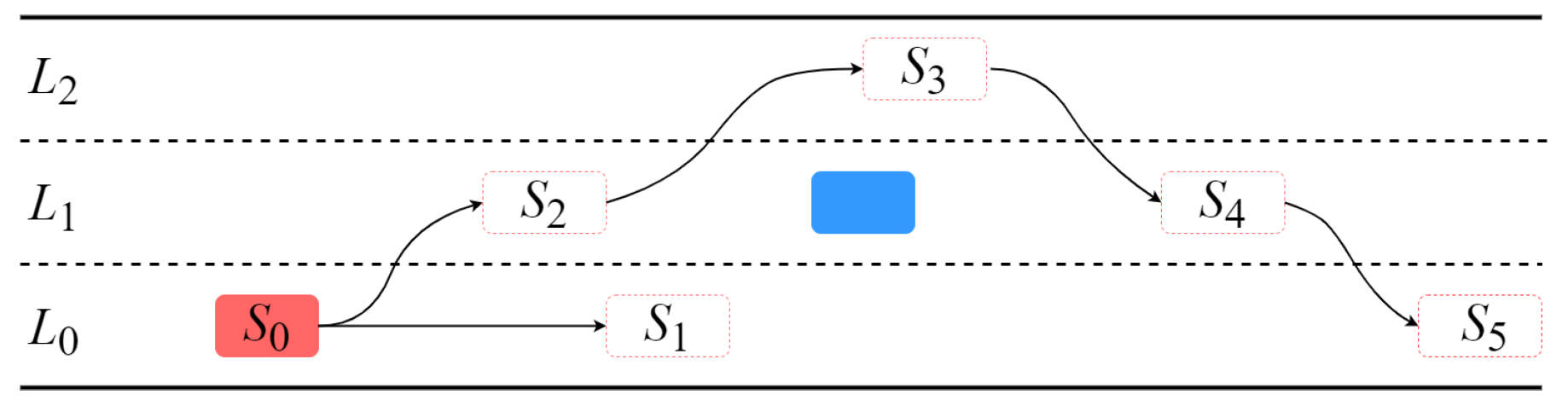
In order to better describe the maneuver and trajectory planning, the two possible scenarios are divided into six stages: $S_0$, $S_1$, $S_2$, $S_3$, $S_4$, and $S_5$, as shown in Figure 5. $S_0$ is the initial stage. In stages $S_0$ and $S_1$, car-following is realized ($S_0\to S_1$). The overtaking consists of stages $S_0$, $S_2$, $S_3$, $S_4$, and $S_5$ ($S_0\to S_2\to S_3\to S_4\to S_5$). In these stages, the OV is always in the middle lane $L_1$, while the EV drives in different lanes. In detail:

• $S_0$: The EV is driving behind the OV in $L_0$ with a greater longitudinal velocity.
• $S_1$: The EV is following the OV in $L_0$ with a smaller longitudinal velocity.
• $S_2$: The EV is driving in lane $L_1$, waiting for a chance to change to $L_2$. This is a transition stage.
• $S_3$: The EV reaches lane $L_2$ and drives in $L_2$ before overtaking the OV from the left, looking for an opportunity to go back to lane $L_1$. In this stage, lane keeping also occurs.
• $S_4$: The EV reaches lane $L_1$, and is preparing for moving to lane $L_0$.
• $S_5$: The EV drives in lane $L_0$.

4.2. Maneuver Planning

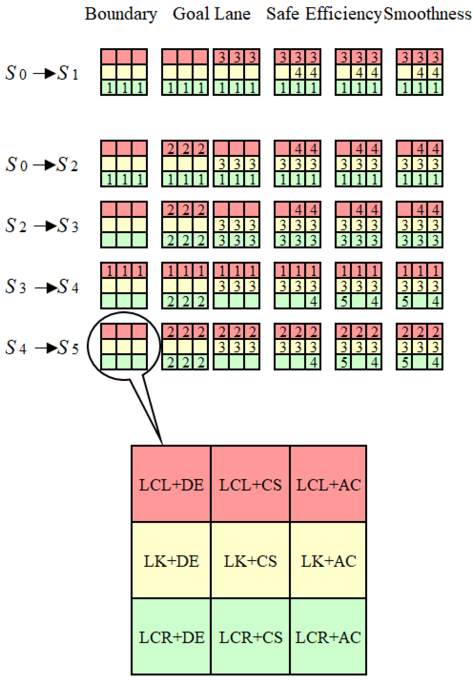
The procedure of maneuver selection is shown in Figure 6. The box represents the nine possible combinations of maneuvers in the lateral and longitudinal directions. The tiny cubes without numbers on them stand for current candidate maneuvers. The tiny cubes with numbers inside represent the maneuvers that are excluded from the candidate maneuvers. The numbers, ‘1’, ‘2’, ‘3’, ‘4’, ‘5’, and ‘6’, represent the reasons for removing maneuvers. Among them, ‘1’, ‘2’, and ‘3’ are for removing lateral maneuvers, and ‘4’, ‘5’, and ‘6’ are the reasons for removing longitudinal maneuvers. They stand for:

• 1—The vehicle will reach the edge of the road if it turns left (or right).
• 2—The goal is to change lane but the the safety constraints for changing lane is not satisfied.
• 3—By conducting these maneuvers, the vehicle cannot move to the target lane even though the conditions for changing lane are fulfilled.
• 4—These maneuvers contribute less/nothing to increasing TTC and TIV.
• 5—These maneuvers contribute less to improving efficiency.
• 6—Selecting these maneuvers has a negative or no positive impact on smoothness of driving behaviors.

In the following, we explain how the proposed maneuver selection method works in the two possible scenarios, the car-following scenario and the overtaking scenario.

4.2.1. Maneuver Selection in Car-Following Scenario: $S_0\to S_1$

Following the OV in the current lane is an excessively conservative but feasible choice in terms of collision avoidance. To implement the maneuver selection, one maneuver will be selected from all possible maneuvers in each direction. The lateral maneuver is first selected. Changing to the right lane (LCR) is excluded because of the boundary constraints. Then, we remove changing to the left lane (LCL) because it is inconsistent with current goal scenario (car-following), so only lane keeping (LK) is left. Finally, longitudinally, both TTC and TIV will definitely decrease if keeping the current speed (CS) or accelerating (AC), but decelerating (DE) probably causes an increase in TTC and TIV, so decelerating is selected as a longitudinal maneuver. Combining the results of maneuver selection in both directions, we obtain the LK+DE maneuver for this car-following scenario.

4.2.2. Maneuver Selection in Overtaking Scenario: $S_0\to S_2\to S_3\to S_4\to S_5$

Overtaking, although highly efficient for the EV, will increase the risk of collision with other traffic participants and requires a careful trajectory design. The stage sequence $S_0\to S_2\to S_3\to S_4\to S_5$ can be divided into four steps: (i) $S_0\to S_2$, (ii) $S_2\to S_3$, (iii) $S_3\to S_4$, and (iv) $S_4\to S_5$.

Note that the target lane of each stage change is not the current lane. In contrast to car-following, the EV now has to examine the environment to judge whether the conditions for changing lanes are satisfied. If not, the EV has to stay in its current lane and wait. The only difference to the maneuver selection procedure in car-following is that now the lane change condition is taken into account.

We do not use TTC and TIV in stage $S_3$, where the EV and OV are in different lanes, because this configuration is safe in the lateral direction. However, the distance in the longitudinal direction might be small, leading to small TTC and TIV, which is a false risk indicator (see discussion in Section 2.2).

4.3. MPC-Based Trajectory Control

The maneuvers selected from the maneuver planning are delivered to the MPC controller for trajectory control. In order to validate our combined maneuver planning and MPC-based trajectory control method, we simulate the overtaking scenario shown in Figure 5.

The parameters of the road and vehicle, the limits of speed and acceleration, the parameters of the safety constraints, the prediction horizon, the sampling time, and the weighting matrices are set to:

$$\begin{array}{cc}\hfill & w_{\mathrm{lane}}=5.25\mathrm{m},w_{\mathrm{veh}}=1.83\mathrm{m},\hfill \\ \hfill & v_{x_{\min }}=13.6\mathrm{m}/\mathrm{s},v_{x_{\max }}=70\mathrm{m}/\mathrm{s},\hfill \\ \hfill & a_{x_{\min }}=-9\mathrm{m}/\mathrm{s}{}^2,a_{x_{\max }}=6\mathrm{m}/\mathrm{s}{}^2,\hfill \\ \hfill & a_{y_{\min }}=-0.5\mathrm{m}/\mathrm{s}{}^2,a_{y_{\max }}=0.5\mathrm{m}/\mathrm{s}{}^2,\hfill \\ \hfill & a=5\mathrm{m},b=2.625\mathrm{m},\hfill \\ \hfill & N=25,T=0.2.\hfill \\ \hfill & q_1=1,q_2=0.1,\hfill \\ \hfill & r_1=0,r_2=10,r_3=100,r_4=0,\hfill \\ \hfill & s_1=0,s_2=10,s_3=100,s_4=0.\hfill \end{array}$$

(15)

The initial positions of both vehicles are shown in Figure 7.

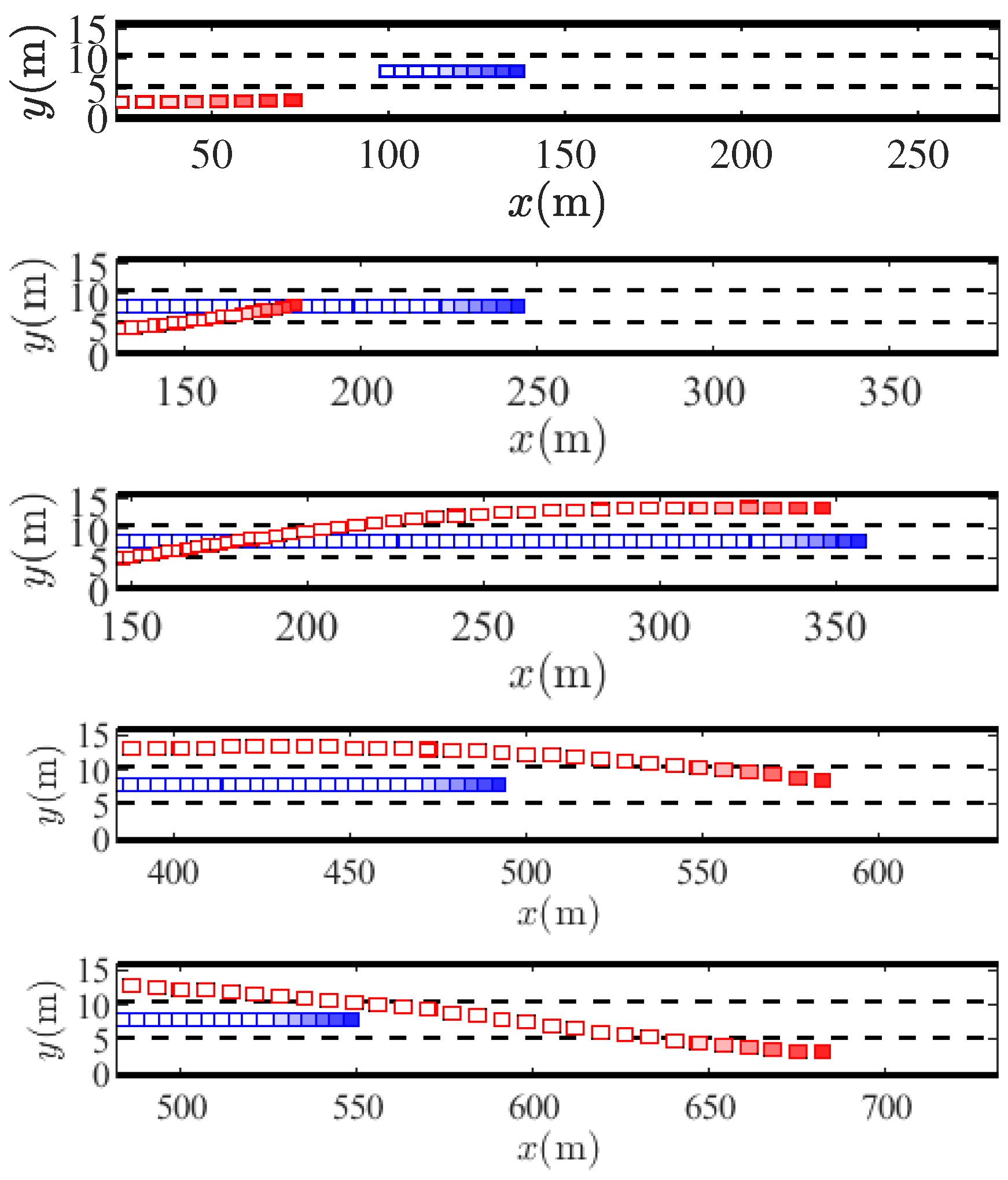
From Section 4.1, we know that there are five stages and four stage changes in the overtaking scenario, as shown in Figure 5. The simulation results of our combined maneuver planning and MPC-based trajectory control method are shown in Figure 8. The successive five figures show the five stages in the overtaking scenario: $S_0$, $S_2$, $S_3$, $S_4$, $S_5$.

In Figure 8, the dark red rectangle is the current position of the EV, and the other red rectangles stand for the past trajectory of the EV. Similarly, the dark blue rectangle is the current position of the OV, and all other blue rectangles indicate the trajectory of the OV.

The maneuvers that the EV selects can also be extracted from Figure 8. The lateral maneuvers can be observed directly from the lateral positions of the EV (red). The changes of density of the rectangles indicate the longitudinal maneuvers. When the density of the rectangles in a trajectory changes from sparse to dense, the vehicle executes a deceleration maneuver, and vice versa. In addition, no change in the longitudinal distance between rectangles implies that the vehicle drives at a constant longitudinal velocity.

5. Conclusions

In this paper, we propose a maneuver selection method which chooses one maneuver from all potential ones by excluding less appropriate maneuvers based on five rules involving lane edges, the goal lane, safety, efficiency, and smoothness. Furthermore, an MPC-based trajectory generation method is used to execute the selected maneuver by designing a corresponding cost function and constraints for the MPC controller.

We validate the proposed method for an overtaking scenario on a three-lane highway. The whole overtaking scenario can be divided into five stages. The results show that at each stage, the ego vehicle can successfully reach the desired lane, conduct the desired speed maneuver, and avoid collisions.

Our current maneuver planning method is executed at each time step, which allows the autonomous vehicle to rapidly adjust its behavior in risky situations. However, the high frequency of updating also causes unnecessary computational burden when the driving environment is mostly safe. Therefore, a trade-off between ensuring fast response when necessary and avoiding unnecessary computation should be achieved in future work.

References

- Menéndez-Romero, C.; Winkler, F.; Dornhege, C.; Burgard, W. Maneuver planning for highly automated vehicles. In Proceedings of the 2017 IEEE Intelligent Vehicles Symposium (IV), Los Angeles, CA, USA, 11–14 June 2017; pp. 1458–1464. [Google Scholar]
- Chen, C.; Gaschler, A.; Rickert, M.; Knoll, A. Task planning for highly automated driving. In Proceedings of the 2015 IEEE Intelligent Vehicles Symposium (IV), Seoul, Korea, 28 June–1 July 2015; pp. 940–945. [Google Scholar]
- Ferguson, D.; Howard, T.M.; Likhachev, M. Motion planning in urban environments. J. Field Robot. 2008, 25, 939–960. [Google Scholar] [CrossRef]
- González, D.; Pérez, J.; Milanés, V.; Nashashibi, F. A Review of Motion Planning Techniques for Automated Vehicles. IEEE Trans. Intell. Transp. Syst. 2016, 17, 1135–1145. [Google Scholar] [CrossRef]
- Paden, B.; Čáp, M.; Yong, S.Z.; Yershov, D.; Frazzoli, E. A Survey of Motion Planning and Control Techniques for Self-Driving Urban Vehicles. IEEE Trans. Intell. Veh. 2016, 1, 33–55. [Google Scholar] [CrossRef] [Green Version]
- Glaser, S.; Vanholme, B.; Mammar, S.; Gruyer, D.; Nouvelière, L. Maneuver-Based Trajectory Planning for Highly Autonomous Vehicles on Real Road With Traffic and Driver Interaction. IEEE Trans. Intell. Transp. Syst. 2010, 11, 589–606. [Google Scholar] [CrossRef]
- Wang, D.; Qi, F. Trajectory planning for a four-wheel-steering vehicle. In Proceedings of the 2001 ICRA, IEEE International Conference on Robotics and Automation (Cat. No.01CH37164), Seoul, Korea, 21–26 May 2001; IEEE: Piscataway, NJ, USA, 2001; Volume 4, pp. 3320–3325. [Google Scholar]
- Frazzoli, E.; Dahleh, M.A.; Feron, E. Maneuver-based motion planning for nonlinear systems with symmetries. IEEE Trans. Robot. 2005, 21, 1077–1091. [Google Scholar] [CrossRef]
- Kushleyev, A.; Likhachev, M. Time-bounded lattice for efficient planning in dynamic environments. In Proceedings of the 2009 IEEE International Conference on Robotics and Automation, Kobe, Japan, 12–17 May 2009; pp. 1662–1668. [Google Scholar]
- Fraichard, T.; Scheuer, A. From Reeds and Shepp’s to continuous-curvature paths. IEEE Trans. Robot. 2004, 20, 1025–1035. [Google Scholar] [CrossRef] [Green Version]
- Petrov, P.; Nashashibi, F. Modeling and Nonlinear Adaptive Control for Autonomous Vehicle Overtaking. IEEE Trans. Intell. Transp. Syst. 2014, 15, 1643–1656. [Google Scholar] [CrossRef] [Green Version]
- Piazzi, A.; Lo Bianco, C.G.; Bertozzi, M.; Fascioli, A.; Broggi, A. Quintic G/sup 2/-splines for the iterative steering of vision-based autonomous vehicles. IEEE Trans. Intell. Transp. Syst. 2002, 3, 27–36. [Google Scholar] [CrossRef]
- Rastelli, J.P.; Lattarulo, R.; Nashashibi, F. Dynamic trajectory generation using continuous-curvature algorithms for door to door assistance vehicles. In Proceedings of the 2014 IEEE Intelligent Vehicles Symposium Proceedings, Dearborn, MI, USA, 8–11 June 2014; pp. 510–515. [Google Scholar]
- Berglund, T.; Brodnik, A.; Jonsson, H.; Staffanson, M.; Soderkvist, I. Planning Smooth and Obstacle-Avoiding B-Spline Paths for Autonomous Mining Vehicles. IEEE Trans. Autom. Sci. Eng. 2010, 7, 167–172. [Google Scholar] [CrossRef] [Green Version]
- Dijkstra, E. A note on two problems in connexion with graphs. Numer. Math. 1959, 1, 269–271. [Google Scholar] [CrossRef] [Green Version]
- Bohren, J.; Foote, T.; Keller, J.; Kushleyev, A.; Lee, D.; Stewart, A.; Vernaza, P.; Derenick, J.; Spletzer, J.; Satterfield, B. Little Ben: The Ben Franklin Racing Team’s Entry in the 2007 DARPA Urban Challenge. In The DARPA Urban Challenge; Springer: Berlin/Heidelberg, Germany, 2009; pp. 231–255. [Google Scholar]
- Hart, P.E.; Nilsson, N.J.; Raphael, B. A Formal Basis for the Heuristic Determination of Minimum Cost Paths. IEEE Trans. Syst. Sci. Cybern. 1968, 4, 100–107. [Google Scholar] [CrossRef]
- Wang, Q.; Ayalew, B.; Weiskircher, T. Predictive Maneuver Planning for an Autonomous Vehicle in Public Highway Traffic. IEEE Trans. Intell. Transp. Syst. 2019, 20, 1303–1315. [Google Scholar] [CrossRef]
- Kogan, D.; Murray, R.M. Optimization-Based Navigation for the DARPA Grand Challenge. In Proceedings of the 45th Conference on Decision and Control (CDC), San Diego, CA, USA, 13–15 December 2006; p. 6. [Google Scholar]
- Dolgov, D.; Thrun, S.; Montemerlo, M.; Diebel, J. Path Planning for Autonomous Vehicles in Unknown Semi-structured Environments. Int. J. Robot. Res. 2010, 29, 485–501. [Google Scholar] [CrossRef]
- Ziegler, J.; Bender, P.; Dang, T.; Stiller, C. Trajectory planning for Bertha—A local, continuous method. In Proceedings of the 2014 IEEE Intelligent Vehicles Symposium Proceedings, Dearborn, MI, USA, 8–11 June 2014; pp. 450–457. [Google Scholar]
- Elbanhawi, M.; Simic, M. Sampling-Based Robot Motion Planning: A Review. IEEE Access 2014, 2, 56–77. [Google Scholar] [CrossRef]
- Kuwata, Y.; Teo, J.; Fiore, G.; Karaman, S.; Frazzoli, E.; How, J.P. Real-Time Motion Planning With Applications to Autonomous Urban Driving. IEEE Trans. Control Syst. Technol. 2009, 17, 1105–1118. [Google Scholar] [CrossRef]
- Yoon, J.; Crane, C.D. Path planning for Unmanned Ground Vehicle in urban parking area. In Proceedings of the 2011 11th International Conference on Control, Automation and Systems, Gyeonggi-do, Korea, 26–29 October 2011; pp. 887–892. [Google Scholar]
- Kong, J.; Pfeiffer, M.; Schildbach, G.; Borrelli, F. Kinematic and dynamic vehicle models for autonomous driving control design. In Proceedings of the 2015 IEEE Intelligent Vehicles Symposium (IV), Seoul, Korea, 28 June–1 July 2015; pp. 1094–1099. [Google Scholar]
- Anderson, S.J.; Peters, S.C.; Pilutti, T.E.; Iagnemma, K. An optimal-control-based framework for trajectory planning, threat assessment, and semi-autonomous control of passenger vehicles in hazard avoidance scenarios. Int. J. Veh. Auton. Syst. 2010, 8, 190–216. [Google Scholar] [CrossRef]
- Bhargav, J.; Betz, J.; Zehng, H.; Mangharam, R. Deriving Spatial Policies for Overtaking Maneuvers with Autonomous Vehicles. In Proceedings of the 2022 14th International Conference on COMmunication Systems NETworkS (COMSNETS), Bengaluru, India, 4–8 January 2022; pp. 859–864. [Google Scholar] [CrossRef]
- Musa, A.; Pipicelli, M.; Spano, M.; Tufano, F.; De Nola, F.; Di Blasio, G.; Gimelli, A.; Misul, D.A.; Toscano, G. A Review of Model Predictive Controls Applied to Advanced Driver-Assistance Systems. Energies 2021, 14, 7974. [Google Scholar] [CrossRef]
- Hayward, J.C. Near-Miss Determination through Use of a Scale of Danger; University Park, Pa, Pennsylvania Transportation and Traffic Safety Center, The Pennsylvania State University: State College, PA, USA, 1972. [Google Scholar]
- Pendleton, S.D.; Andersen, H.; Du, X.; Shen, X.; Meghjani, M.; Eng, Y.H.; Rus, D.; Ang, M.H. Perception, Planning, Control, and Coordination for Autonomous Vehicles. Machines 2017, 5, 6. [Google Scholar] [CrossRef]
- Brüdigam, T.; Olbrich, M.; Wollherr, D.; Leibold, M. Stochastic Model Predictive Control with a Safety Guarantee for Automated Driving. IEEE Trans. Intell. Veh. 2021, 1. [Google Scholar] [CrossRef]
- Katrakazas, C.; Quddus, M.; Chen, W.H.; Deka, L. Real-time motion planning methods for autonomous on-road driving: State-of-the-art and future research directions. Transp. Res. Part C Emerg. Technol. 2015, 60, 416–442. [Google Scholar] [CrossRef]
- Rawlings, J.; Mayne, D.; Diehl, M. Model Predictive Control: Theory, Computation, and Design; Nob Hill Publishing: Madison, WI, USA, 2017. [Google Scholar]
- Brüdigam, T.; Olbrich, M.; Leibold, M.; Wollherr, D. Combining Stochastic and Scenario Model Predictive Control to Handle Target Vehicle Uncertainty in an Autonomous Driving Highway Scenario. In Proceedings of the 2018 21st International Conference on Intelligent Transportation Systems (ITSC), Maui, HI, USA, 4–7 November 2018; pp. 1317–1324. [Google Scholar]
- Gao, Y.; Lin, T.; Borrelli, F.; Tseng, E.; Hrovat, D. Predictive Control of Autonomous Ground Vehicles with Obstacle Avoidance on Slippery Roads. In Proceedings of the ASME 2010 Dynamic Systems and Control Conference, Cambridge, MA, USA, 12–15 September 2010; Volume 1. [Google Scholar] [CrossRef] [Green Version]
- Levinson, J.; Askeland, J.; Becker, J.; Dolson, J.; Held, D.; Kammel, S.; Kolter, J.Z.; Langer, D.; Pink, O.; Pratt, V.; et al. Towards fully autonomous driving: Systems and algorithms. In Proceedings of the 2011 IEEE Intelligent Vehicles Symposium (IV), Baden-Baden, Germany, 5–9 June 2011; pp. 163–168. [Google Scholar] [CrossRef]
- Carvalho, A.; Gao, Y.; Gray, A.; Tseng, H.E.; Borrelli, F. Predictive control of an autonomous ground vehicle using an iterative linearization approach. In Proceedings of the 16th International IEEE Conference on Intelligent Transportation Systems (ITSC 2013), The Hague, The Netherlands, 6–9 October 2013; pp. 2335–2340. [Google Scholar] [CrossRef]
- Carvalho, A.; Gao, Y.; Lefevre, S.; Borrelli, F. Stochastic predictive control of autonomous vehicles in uncertain environments. In Proceedings of the 12th International Symposium on Advanced Vehicle Control, Tokyo, Japan, 22–26 September 2014; pp. 712–719. [Google Scholar]
- Brito, B.; Floor, B.; Ferranti, L.; Alonso-Mora, J. Model Predictive Contouring Control for Collision Avoidance in Unstructured Dynamic Environments. IEEE Robot. Autom. Lett. 2019, 4, 4459–4466. [Google Scholar] [CrossRef]
- Jewison, C.; Erwin, R.S.; Saenz-Otero, A. Model Predictive Control with Ellipsoid Obstacle Constraints for Spacecraft Rendezvous. IFAC-PapersOnLine 2015, 48, 257–262. [Google Scholar] [CrossRef]
- Schimpe, A.; Diermeyer, F. Steer with Me: A Predictive, Potential Field-Based Control Approach for Semi-Autonomous, Teleoperated Road Vehicles. In Proceedings of the 2020 IEEE 23rd International Conference on Intelligent Transportation Systems (ITSC), Rhodes, Greece, 20–23 September 2020; pp. 1–6. [Google Scholar] [CrossRef]
Figure 1.
Interconnection of maneuver planning and trajectory tracking.
Figure 2.
Nine feasible combined maneuvers. Boxes with the same color contain three different maneuvers in the longitudinal direction: decelerating (DE), staying at/maintaining current speed (CS), and accelerating (AC). Boxes with different colors represent distinct maneuvers in the lateral direction. The red, yellow, and green boxes illustrate changing to left lane (LCL), keeping/continuing moving in current lane (LK), and changing to right lane (LCR), respectively.
Figure 3.
The maneuver selection method.
Figure 4.
Safe region for a vehicle that is turning left.
Figure 5.
Car-following and overtaking.
Figure 6.
Maneuver Selection: The box displays the 9 possible maneuvers: LCL+DE, LCL+CS, LCL+AC, LK+DE, LK+CS, LK+AC, LCR+DE, LCR+CS, and LCR+AC.
Figure 7.
Initial states of the vehicles.
Figure 8.
Five stages for the overtaking scenario: , , , , .