Novel Multi-Vehicle Motion-Based Model of Trolleybus Grids towards Smarter Urban Mobility

Abstract

Trolleybus systems are resurfacing as a steppingstone to carbon-neutral urban transport. With an eye on smart city evolution, the study and simulation of a proper monitoring system for trolleybus infrastructures will be essential. This paper merges the authors’ engineering knowledge and sources available in the literature on designing and modeling catenary-based electric traction networks and performs a critical review of them to lay the foundations for proposing possible optimal alternatives. A novel multi-vehicle motion-based model of the DC catenary system is then devised and simulated in Matlab-Simulink, which could prove useful in predicting possible technical obstacles arising from the next-future introduction of smart electric traction grids, inevitably featuring greater morphological intricacy. The modularity property characterizing the created model allows an accurate, detailed, and flexible simulation of sophisticated catenary systems. By means of graphical and numerical results illustrating the behavior of the main electrical line parameters, the presented approach demonstrates today’s obsolescence of conventional design methods used so far. The trolleybus network of the city of Bologna was chosen as a case study.

1. Introduction

The reduction of greenhouse gas (GHG) emissions is one of the greatest global challenges through 2050. Aside from GHG emissions, air pollution, such as nitrogen oxide and particulate matter emissions, has gained increasing attention in agglomerated areas, with transport vehicles being one of the main sources thereof [1]. Increasing awareness of climate change and the urgent need to prepare for a post-petrol era have prompted most of the world’s developed countries to investigate alternatives for transport systems that rely more on energy-efficient vehicles. Transportation electrification is anticipated to be a critical future reality of worldwide mobility systems, helping reduce climate change and air quality impacts. Among others, trolleybuses can play a strong part in urban transport for years to come. Trolleybuses are buses that run on electricity provided by overhead wires, giving them the powerful traction inherent in rail modes (e.g., metro and light rail systems). However, unlike these modes, they are cheaper to construct and have greater operational flexibility.

When embarking on a smart city project, the extension and the strengthening of the metropolitan trolleybus electrical infrastructure might become a noteworthy task. In this perspective, a clever integration of renewable energy sources (RES) and stationary energy storage systems (ESSs) within the trolleybus network has a great chance of favoring the deployment of electric vehicles (EVs), forasmuch as the network itself could work as a DC backbone for EV chargers. The same considerations also apply to other forms of catenary-powered urban transport (e.g., tramways and metro) or in general to any existing strategy for dynamic conductive power transfer (e.g., third-rail systems). In this direction, research has been already conducted on railway systems [2]. To prove the viability of such a goal, the development of a circuit model of overhead wire electrical systems in Simulink might stand as a sound candidate, and it is therefore proposed in this work.

With the objective of reducing the environmental impact of public transport in Emilia-Romagna, which is still mainly powered by endothermic engines, the city of Bologna is working on the introduction of In-Motion-Charging (IMC) trolleybuses in the urban transit system. Such innovative trolleybuses are powered by the catenary and equipped with on-board battery storage systems to extend the journeys to non-powered routes. Technical obstacles can be encountered due to the greater absorption of electrical power by the IMC buses to guarantee both the energy for traction and the energy for recharging the batteries to be used for the stretches without a contact line. The proposed catenary system virtual model might be adopted to ensure the project’s feasibility, for which it will be essential to develop control of the energy and power flows to ensure the least impact on the line, maximize efficiency, and reduce possible disruptions to users.

The electrical infrastructure of a typical contact wire-based electric traction network consists mainly of DC traction power substations (TPSSs) (i.e., uncontrolled rectifier substations) and overhead contact line (OCL) systems. To guarantee the regularity of the traction system’s operation, the OCLs are divided into feeding sections (FSs) or electrical zones that are fed separately [3]. An FS is the portion of the OCL between two or more electrical disconnection points. The electrical disconnection points along the OCLs are considered to always be open-circuited, as they are not commonly operable except in case of an emergency. Ordinary FSs are supplied bilaterally. In the event of bidirectional traffic (typically for urban traction grids), the two physically parallel OCLs are connected at different regularly distributed points by equipotential bonding or voltage equalizers, forming a double contact line (or a double-bifilar line in the case of trolleybuses). The equipotentiality achieved by these electrical connections tends to limit the voltage drops along the catenary by reducing the electrical resistance, especially farther from the TPSSs. While a detailed analysis of TPSSs is omitted in this paper, our work explores existing approaches (either implemented for already built infrastructures or proposed in the literature) for the design, verification, and monitoring of the catenary system to ensure service continuity and technical standards compliance. Bologna’s trolleybus network was chosen as a case study, being arranged with FSs with simple (ordinary structure of an electric railway FS) and mainly complex topologies, with the latter emphasizing the potential of our simulation tool. The same network stands as a valid basis to compare the modeling methods discussed here.

To the best of the authors’ knowledge, the methodologies effectively enacted for designing the existing metropolitan trolleybus systems have not been formalized in technical scientific documents, although they are based on rules dictated by the technical expertise acquired in similar fields. By following such rules and relying on the authors’ experience as researchers in the field, it was possible to reconstruct the theory behind the design of Bologna’s trolley grid.

Nonetheless, the published material on analogous applications is certainly retrievable. The authors in [4,5] described a conventional analytical method for OCL voltage drop verification employed for the electrification of railways, but it is also applicable for trolleybus systems. However, the modernization of urban electricity networks makes it inevitable to perform model-based time domain analysis. Hence, proper simulation tools are required for building and examining descriptive network models. In general, the models reported in the literature are implemented using general purpose programming languages, such as Fortran or C, or graphical programming environments, such as Matlab-Simulink or Modelica.

The research in [6,7,8,9,10] delineated a simulation tool written in Fortran aimed at correctly representing urban railway lines. This tool, named Train-sim, has been developed in the past century and validated for electrified subway [7] and tram [8] lines through in-field experimental tests. In [9,10], the Fortran language-based version was compared with Modelica-based and Simulink-based simulators for tramway systems.

Modelica and Simulink are block diagram environments that allow modeling multidomain systems and deploying without writing code. The authors in [10] managed to build a railway system simulator in Simulink with the same model architecture and equations implemented in Modelica. Aside from that, the relevant literature available on Simulink models appears to be relatively vaster. Hence, the proposed paper does not deal with Modelica. As is understandable, the equivalent electric circuit topology depicting the OCL varies with the movement of the vehicles, which draw a certain amount of electric current. Hence, the vehicles split the circuit into branches of variable resistance. One of the main challenges encountered in simulating overhead contact systems is the representation of such time-varying electrical resistance. Simulink provides a block implementing a variable resistor (Variable Resistor blocks) as a current source driven by a voltage measurement. However, this model presents strong criticalities, as the vehicle current absorption is typically modeled with a controlled current generator [11,12,13,14]. Hence, its direct connection with Variable Resistor blocks would form a current-sources-only cut-set, which originates singularities according to the circuit theory. A possible solution is explained in [12], in which the variable resistor is built with a controlled voltage source. The authors in [13,14] developed a catenary model based on switchable series-connected resistors for imitating variable resistors. In [15], the same concept was applied to trolleybus lines, which are topologically more intricate than railway lines, even though the respective vehicle model includes the nonlinearities of the electric drive system, which may lead to excessively burdensome simulations.

Nevertheless, the variability of the number of vehicles typical of the trolleybus system FSs may compromise the modular extensibility of the aforementioned models. In addition, as said earlier, certain FSs of that sort have more complex morphologies (i.e., they are characterized by the simultaneous presence of single- and double-bifilar OCLs), unsymmetrical TPSSs in the case of bilaterally supplied FSs (both in terms of power delivery and position of the respective outgoing feeders, normally of different lengths, with respect to the FS structure), unevenly arranged voltage equalizers, and reinforcing line feeders. In the present work, the effectiveness of the already-cited modeling approaches is analyzed in relation to such features, highlighting the possible limitations of each when applied to trolleybus grids. Such a critical review sets the stage for devising a novel catenary modeling technique in a Simulink environment, where the flexible man–machine interface and the broad variety of functionalities make it versatile and future-proof in a perspective of intelligent trolley grids. A modular catenary model is investigated here for overcoming the limitations explained, enabling the contribution of trolleybus systems to the emergence of smart cities at the same time.

The discussion is arranged as follows. In Section 2, the conventional analytical method applied for verifying the integrity of the Bologna’s trolleybus grid is presented. Section 3 deals with the literature on the catenary simulation tools, directing the attention to the Fortran and Simulink programming environments. In Section 4, our novel multi-vehicle motion-based (MVMB) OCL model is introduced. Focusing on specific routes within two of the FSs Bologna’s traction system is divided into, Section 5 shows how the MVMB modeling approach could be applied for the evaluation of voltage variations along the catenary, as well as the verification of line overloads and overtemperatures. The analysis includes a direct comparison with the conventional method. In Section 6, all the modeling strategies discussed here are set side by side to display their differences and similarities in relation to several aspects. Lastly, the conclusions are drawn in Section 7.

2. Conventional Analytical Approach

The calculations adopted for dimensioning the current trolleybus electrical infrastructure in Bologna follow a method based on the evaluation of the line electrical parameters at the FS macro-level (i.e., each FS is associated with a unique OCL current, temperature, and voltage value). Such values are derived according to precautionary assumptions, which the present work will examine in the next paragraphs.

2.1. Monitoring of Overloads and Overheating

Let us first understand how the conventional method estimates possible overloads and overtemperatures in the overhead lines.

The standard EN 50119 on electric traction overhead contact lines establishes that the single 100-mm² raw copper wire should not carry more than 451 A [3]. Since the standard relates to a continuous operating condition, the vehicle average current absorption I_m is to be used for monitoring possible overloads, which is given by

$$I_m=\frac{1}{t_{bs}}{{\displaystyle \int }}_0^{t_{bs}}{i}_a dt,$$

(1)

where i_a is the line current absorbed by the trolleybus and t_bs is the mean time between stops (with dwelling times at stops included).

The conventional design method resorts to the calculation of a unique total average current I_M, which accounts for the assumed number of vehicles within the affected FS:

$$I_M={{\displaystyle \sum }}_j{I}_{m,j}{N}_j,$$

(2)

where I_m,j is the vehicle average current for the trolleybuses of the jth type and N_j is the number of trolleybuses of jth type inside the FS.

Based on the FS configuration,

Table 1. OCL pole current for overload analysis.

OCL Pole Current		OCL Structure
		Single-Bifilar	Double-Bifilar
Power supply configuration	Unilateral	IM	IM/2
	Bilateral	IM/2	IM/4

collects the formulas for deriving the OCL pole current to be compared with the ampacity threshold imposed by the abovementioned standard. The following simplifying hypotheses explain why the single-wire current is obtained as a divisor of I_M in specific cases:

• Each bilaterally supplied FS is symmetrical in relation to the two TPSSs (i.e., the line feeders leaving the TPSSs are assumed to be of identical lengths (i.e., same voltage drop), and the TPSSs themselves equally share the power delivered to the FS. Therefore, each TPSS supplies half of the line current;
• The two catenary lines constituting the FSs with bidirectional traffic (two-way street or different outward and return routes) are assumed to be electrically in parallel (i.e., the corresponding positive and negative poles are theoretically connected at infinite points along the whole OCL length). This leads to a perfect halving of the line current at any position.

Of course, if an FS satisfies both hypotheses 1 and 2 simultaneously, the OCL pole current is given by a quarter of I_M.

Keeping the maximum current in the conductors within the specified limits is a primary objective in the design of OCLs, which could otherwise be damaged by excessive heating. The standard EN 50119 also states that the maximum temperature rise in the OCL conductors should not lead to conductor temperatures above 80 °C in steady state conditions [3]. With a good approximation, the OCL pole temperature θ_OCL is governed by the following differential equation:

$${\tau }_{th}\frac{d{\theta }_{OCL}}{dt}+\left({\theta }_{OCL}-{\theta }_{OCL,0}\right)=C{\sigma }^2=C{\left(\frac{I_{OCL}}{S_{OCL}}\right)}^2,$$

(3)

where τ_th is the thermal time constant of the system, θ_OCL,0 is the initial temperature, C is the heat constant (°C mm⁴/A²), σ (A/mm²) is the electric current density, I_OCL is the OCL pole current, and S_OCL (mm²) is the cross-section of the OCL conductor. To verify the compliance with the aforementioned standard, the analysis is limited to the evaluation of the steady state temperature θ_OCL,ss, obtained from Equation (3):

$${\dot{\theta }}_{OCL}=0\to {\theta }_{OCL,ss}=C{\sigma }^2=C{\left(\frac{I_{OCL}}{S_{OCL}}\right)}^2+{\theta }_{OCL,0}.$$

(4)

Generally, the thermal transients of the OCLs are governed by a time constant τ_th that has a much longer duration than current start-up transients. As a consequence, θ_OCL,ss may be studied with reference to the vehicle average current absorption, which means that in the conventional approach, we resort to the overall average current I_M. According to the FS configuration, I_OCL in Equation (2) is expressed with the relative formula in Table 1.

2.2. Probability-Based Calculation of the Line Voltage Drop

Given the electrical resistance per unit length and the distance between TPSSs, it is possible to calculate the voltage drops corresponding to a certain line’s current consumption. This voltage varies according to the position of the vehicles and the currents absorbed by them.

The correct functioning of the electrical infrastructure requires that the line voltage does not fall below a value that the standards set at two-thirds of the nominal voltage (the rated value is 750 V in EN 50163 [16]). Hence, it is necessary to verify the maximum voltage drops corresponding to the heaviest load conditions. For the sake of completeness, the same standard sets the upper line voltage limit to 1000 V; however, overcoming such a threshold is quite unlikely, as the acceleration time of the vehicle between two bus stops prevails over its braking phase duration.

In the following paragraphs, we will consider a line section of length L without intermediate branches, (The points of connections of the feeders with the catenary are placed at its extremities, and no further supply points or reinforcing feeders are included as a cautionary measure.) neglecting for simplicity the internal voltage drops of the TPSSs and therefore considering the voltage at the supply busbars to be constant when the load varies.

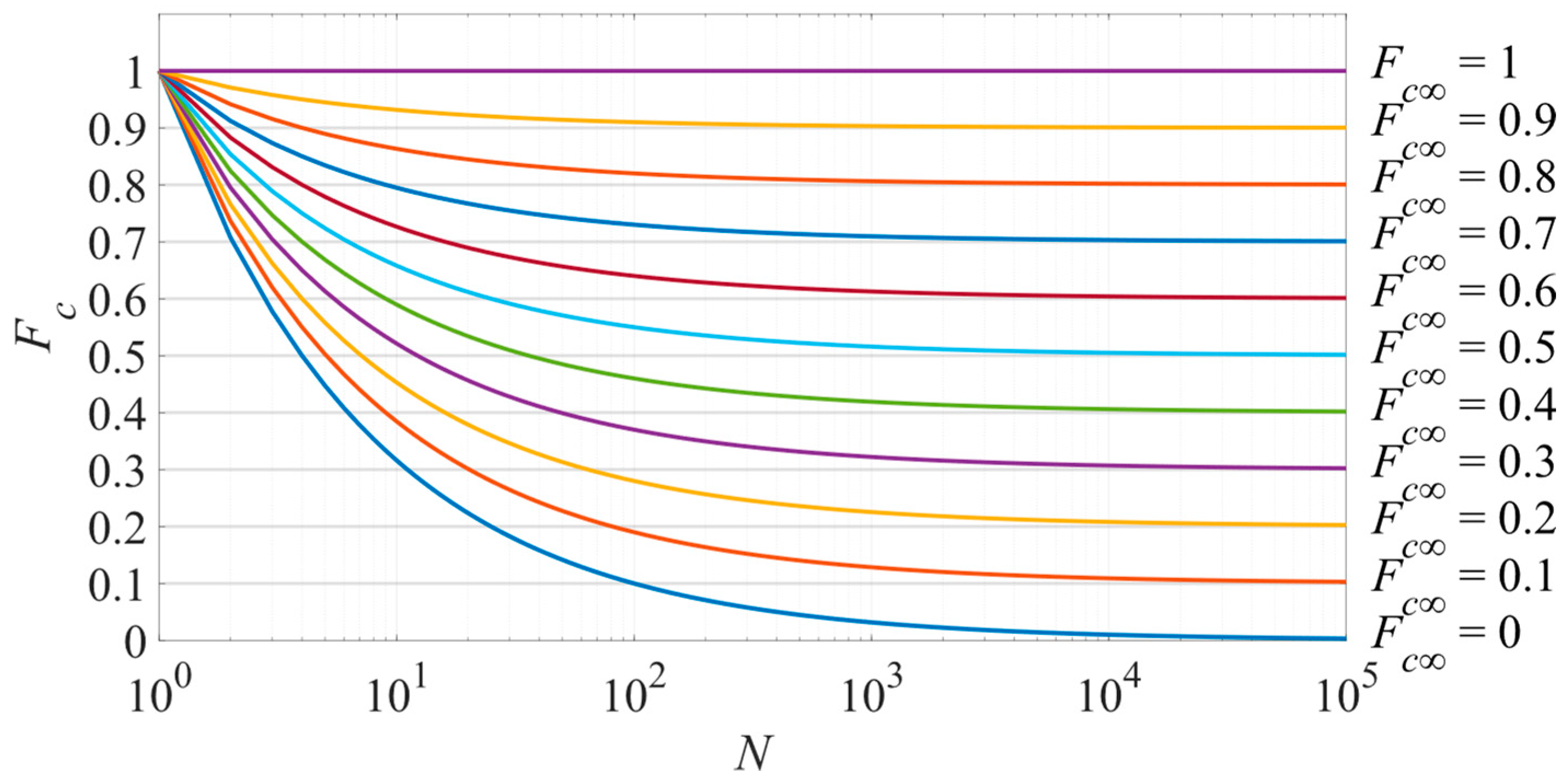
2.2.1. Probabilistic Derivation of the Current Consumption at the Feeding Section Macro-Level

As a precautionary hypothesis, to determine the maximum voltage drop along the catenary, the vehicle starting current I_s is used (i.e., the mean value of the current taken by the traction inverter during the starting period), and it is obtained as follows:

$$I_s=\frac{1}{t_s}{{\displaystyle \int }}_0^{t_s}{i}_a dt>I_m,$$

(5)

where t_s is the start-up time duration (until the maximum speed is reached).

The evaluation of the OCL voltage drops affecting each FS is performed by estimating a total starting current accounting for the number of vehicles within each FS per each vehicle type. As it is requested to calculate the maximum voltage drop, the representation of a worst-case scenario is of interest. Such a scenario is characterized by trolleybuses working in the phase of the highest line current absorption (i.e., the start-up phase). With reference to the procedure adopted by Rusck [17] (re-examined in [18]), the start-up time durations of vehicles of the same type are assumed to be normally distributed. Given the jth trolleybus type, the start-up coincidence (or simultaneity) factor that a very large number of vehicles would have is calculated as follows:

$$F_{c\infty ,j}=\frac{t_{s,j}}{t_{bs,j}},$$

(6)

where t_s,j is the start-up time duration for the trolleybuses of the jth type and t_bs,j is the mean time between stops for the trolleybuses of the jth type. Ideally, given a set of an infinite number of similar vehicles, this factor represents the probability of each vehicle to be in the starting phase at each instant. Because the time between stops is always larger or equal to the start-up time duration, the calculated simultaneity factor always varies between zero and one.

Since an FS may be characterized by the presence of different trolleybuses at the same time, we must resort to the mean coincidence factor, which is always obtained as follows with the hypothesis of a large number of vehicles for each jth type:

$$F_{c\infty ,m}=\frac{{{\displaystyle \sum }}_j{F}_{c\infty ,j}{N}_j}{{{\displaystyle \sum }}_j{N}_j}=\frac{{{\displaystyle \sum }}_j{F}_{c\infty ,j}{N}_j}{N},$$

(7)

where N is the total number of buses moving inside the FS.

In practice, when dealing with a common finite number of vehicles present within an FS, the expression of the start-up coincidence factor becomes [17,18,19,20,21,22,23]

$$F_c=F_{c\infty ,m}+\frac{1-F_{c\infty ,m}}{\sqrt{N}}.$$

(8)

Therefore, from Equation (8), the total starting current drawn by the vehicles inside the FS is calculated as follows:

$$I_S=F_c{{\displaystyle \sum }}_j{I}_{s,j}{N}_j=\left(F_{c\infty ,m}+\frac{1-F_{c\infty ,m}}{\sqrt{N}}\right){{\displaystyle \sum }}_j{I}_{s,j}{N}_j,$$

(9)

where I_s,j is the starting current drawn by a trolleybus of the jth type.

Focusing, for the sake of simplicity, on the case of trolleybuses with identical characteristics (i.e., F_c∞,m = F_c∞), the relationship between the simultaneity factor and the number of vehicles for different values of F_c∞ is depicted in Figure 1. Note that the horizontal axis has a logarithmic scale. The figure shows that the coincidence factor decreases with the increasing number of considered trolleybuses, as it becomes less probable that they are in their start-up phase simultaneously. For a very large number of vehicles, the coincidence factor F_c is very close to the respective value taken by F_c∞.

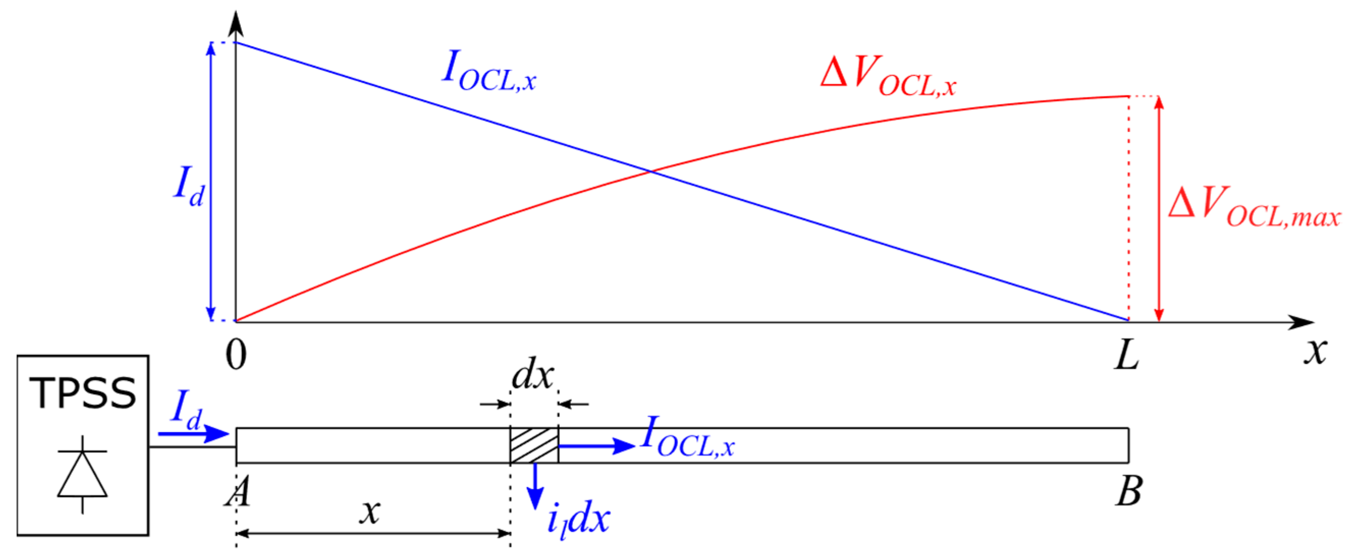
2.2.2. Voltage Drop Evaluation with a Unilateral Power Supply

It is assumed that the line section AB is fed at the A end.

(a)

Uniformly distributed load

Let us refer to Figure 2 for the evaluation of the maximum OCL voltage drop in the case of unilaterally supplied FSs.

If the number of trolleybuses becomes very large (the typical case of a high-traffic trolleybus line with low-powered vehicles following one another closely), we are approaching, at the limit, the theoretical situation of a uniformly distributed load, corresponding to a specific current absorption (assuming vehicles having equal characteristics):

$$i_l=\frac{I_d}{L},$$

(10)

where I_d is the total current delivered by the TPSS at line end A.

The load absorption in a line segment of length dx equals

$$d{I}_d=i_{l}dx.$$

(11)

At a distance x from the TPSS, the OCL current is given by

$$I_{OCL,x}=I_d-x{i}_l=\left(L-x\right)i_l.$$

(12)

The voltage drop in the elementary line section considered is obtained as follows:

$$d\left(\Delta V_{OCL,x}\right)=r_l{I}_{OCL,x}dx=r_l\left(L-x\right)i_{l}dx,$$

(13)

where r_l is the OCL electrical resistance per unit length.

Integrating Equation (13) along the line section of length x gives

$$\Delta V_{OCL,x}={{\displaystyle \int }}_0^x{r}_l\left(L-x\right)i_{l}dx=r_l{i}_{l}x\left(L-\frac{x}{2}\right).$$

(14)

Equation (14) shows that ΔV_OCL,x varies with quadratic law as a function of x, and it assumes the maximum value at line end B (see Figure 2) (i.e., for x = L), as expressed in the following formula:

$$\Delta V_{OCL,L}=\Delta V_{OCL,max}=r_l{i}_l\frac{L^2}{2}=r_{l}L\frac{I_d}{2}.$$

(15)

(b)

Evenly spaced concentrated loads

In practice, the catenary is burdened with a finite number of trolleybuses, which can be treated as concentrated loads absorbing the currents I₁, I₂, …, I_N at distances x₁ < x₂ < … < x_N from the TPSS at point A. The maximum voltage drop at the x_N points can be determined as follows by superposition of the effects:

$$\Delta V_{OCL,max}=r_l{\displaystyle \sum }_{h=1}^N{x}_h{I}_h.$$

(16)

Since the exact positions of the vehicles are not known a priori, they are assumed to be evenly spaced from an electrical perspective with respect to the supply points and as far as possible from them so as to represent a more precautionary scenario. For example, if the load is concentrated on a single point, this point is considered to be the farthest end from the TPSS, while if the load is concentrated on two points, half is considered to be on the farthest end from the TPSS, and half in the center, and so on.

In this work, the computation of the maximum OCL voltage drop is performed based on a plus factor ranging between 1 and 2, which depends solely on the number of vehicles N inside the FS. The plus factor is represented in Figure 3 for both unilaterally (k_u) and bilaterally (k_b) fed FSs. By increasing the number of vehicles, the plus factor decreases, as the load is shared among more line points.

In the case of unilaterally supplied FSs, the voltage drop plus factor is determined as follows:

$$\begin{array}{cc}{k}_u=1+\frac{1}{N}=\frac{N+1}{N}& \forall N\in \mathbb{N}\end{array}.$$

(17)

The plus factor-based method provides a compact expression for evaluating the voltage drop, replacing the summation typical of the superposition principle (see Equation (16)), which becomes cumbersome when the number of trolleybuses is relatively large. The maximum voltage drop is hence expressed as follows:

$$\Delta V_{OCL,max,u}=k_u\Delta V_{OCL,max}=\frac{N+1}{N}{r}_{l}L\frac{I_d}{2},$$

(18)

where I_d takes the value of the total starting current I_S. Note that for a very large number of vehicles, with k_u being closer to 1, ΔV_OCL,max,u assumes the result expressed by Equation (15) (i.e., we approach the condition of a uniformly distributed load).

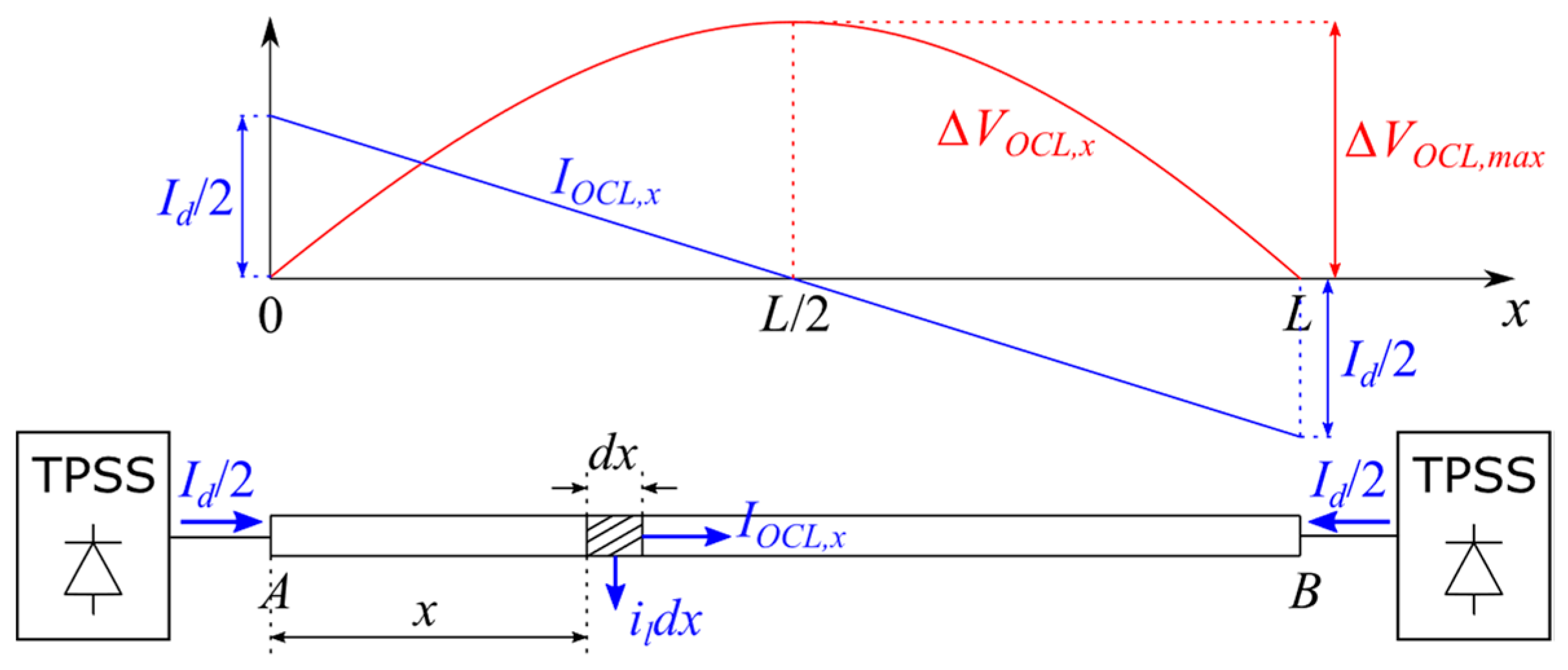
2.2.3. Voltage Drop Evaluation with a Bilateral Power Supply

Let us assume that for both TPSSs, located at the A and B extremities of the line section, the voltage is equal to V_OCL = V_OCL,A = V_OCL,B.

(a)

Uniformly distributed load

Let us refer to Figure 4 for the evaluation of the maximum OCL voltage drop in the case of a bilaterally supplied FS.

Similar to the one-sided supply, the current consumption per unit length (i_l) is given by Equation (10). According to assumption 1 in Section 2.1, each TPSS delivers a current equal to I_d/2 = i_l·L/2. At a distance x from the TPSS, the OCL current is given by

$$I_{OCL,x}=\frac{I_d}{2}-x{i}_l=\left(\frac{L}{2}-x\right)i_l.$$

(19)

The infinitesimal voltage variation at the line segment of length dx is equal to

$$d\left(\Delta V_{OCL,x}\right)=r_l{I}_{OCL,x}dx=r_l\left(\frac{L}{2}-x\right)i_{l}dx,$$

(20)

which, once integrated over the entire OCL section, gives

$$\Delta V_{OCL,x}={{\displaystyle \int }}_0^x{r}_l\left(L-x\right)i_{l}dx=r_l{i}_{l}x\left(\frac{L}{2}-\frac{x}{2}\right).$$

(21)

Additionally, in this case, ΔV_OCL,x varies with quadratic law as a function of x, but this time it takes the maximum value at the midpoint of the OCL section (i.e., for x = L/2). The following result is achieved:

$$\Delta V_{OCL,L/2}=\Delta V_{OCL,max}=r_l{i}_l\frac{L^2}{8}=r_{l}L\frac{I_d}{8}.$$

(22)

(b)

Evenly spaced concentrated loads

In the case of bilaterally supplied FSs, the precautionary assumption of evenly spaced trolleybuses along the catenary is still valid. In this case, if the load is concentrated on a single point, that point is considered to be in the center of the FS, whereas if the load is concentrated on two points, half of it is considered to be at one third of the FS and half is at two thirds, and so on. The voltage drop plus factor is hence obtained as follows (see Figure 3):

$$\begin{array}{cc}{k}_b=\frac{{\left(-1\right)}^N+3+2N}{{\left(-1\right)}^N+1+2N}& \forall N\in \mathbb{N}\end{array}.$$

(23)

Therefore, an expression for the maximum line voltage drop is provided below:

$$\Delta V_{OCL,max,b}=k_b\Delta V_{OCL,max}=\frac{{\left(-1\right)}^N+3+2N}{{\left(-1\right)}^N+1+2N}{r}_{l}L\frac{I_d}{8},$$

(24)

where I_d = I_S. Similar to the previous case, for a very large number of vehicles, ΔV_OCL,max,b, assumes the result expressed by Equation (22).

Since the conventional method relies on the assumption of equality between the currents flowing through the positive and negative OCL poles, one can infer that all the current delivered by the TPSSs runs into the OCL and is eventually drawn by the vehicles. Consequently, no ground current is considered or therefore calculated. Furthermore, with the resistances of the positive and negative poles being equal and traversed by the same current, the circuit may be simplified by virtually bringing the negative wire resistance to the positive wire (disregarding the negative wire), thus obtaining r_l as twice the pole resistance per unit length.

3. Literature on the Simulation Tools

3.1. Fortran Language-Based Model

Let us analyze the simulation tool named Train-sim, which is written in the Fortran language and has been employed for modeling DC railway systems so far. Train-sim consists of two computational codes: Train-perf and Train-el.

The Train-perf calculation code takes the line features and the electromechanical characteristics of the vehicles as input data and outputs the motion profiles of the vehicles themselves. Different traffic scenarios can be determined.

The Train-el code builds an equivalent electrical network for each simulation time step based on the corresponding vehicle positions given by the Train-perf tool. It then executes load flow analysis by assuming the TPSSs, vehicles, and voltage equalizers as electrical nodes, while the resistive branches between such nodes represent the traction circuit stretches with their equivalent resistances.

By adopting classic iterative numerical methods (e.g., Newton–Raphson), the software provides the output powers from each TPSS, the OCL voltage profiles, and the currents flowing through the line feeders. The vehicles are modeled as constant power loads. If the current absorption attempts to exceed the maximum permitted value, such a value is imposed as a constraint during the iterative calculation of the non-linear equations until the voltage seen by the vehicle decreases.

Furthermore, the maximum recuperable powers during the braking phase of the vehicles are computed. If the system allows it, the catenary can accept all the power produced during regenerative braking according to the solution of the system equations. If the voltage increases, the recoverable energy transferred to the OCL diminishes (the portion of energy dissipated on the braking rheostat rises) up to zero (i.e., as soon as the voltage reaches the maximum permitted value).

Even though Train-sim seems to be suitable for covering any simulation scenario, the required coding abilities make it less straightforward to use, as will be discussed later.

3.2. Variable Resistor-Based Catenary Modeling Using Simulink

In the following, we focus on electric traction network modeling in Simulink decoupled from the representation of the vehicle dynamics. Specifically, the catenary behavior may be reasonably simulated by assuming the vehicles to be controlled current sources. These current sources are positioned at fixed points in the line circuit, thus splitting the FS into OCL branches. Hence, the circulation of the vehicles is emulated by changing the OCL equivalent circuit configuration (i.e., the electrical resistances associated with the corresponding OCL branches vary over time based on the motion profiles of the vehicles themselves). As mentioned in Section 1, if such modeling strategies are applied, there is no module in Simulink viable for representing the line resistance variability according to the vehicle position. Two published techniques for emulating the functioning of the variable resistor in railway grids are reported below.

The first strategy consists of inserting a current-controlled voltage source within the OCL section run by the vehicle [12], which is connected in series with an ammeter measuring the line current. By keeping track of the vehicle position, the voltage value assumed by the controlled generator is evaluated as the product of the OCL resistance per unit length, the distance between the vehicle itself and the adjacent TPSS feeding that section, and the measured OCL current. The coefficient of proportionality between the voltage source value and the ammeter reading is the amount of resistance to be attributed to the variable resistor. Nevertheless, it should be stressed that such a formulation requires management of the initial conditions to avoid an unphysical representation (e.g., the short circuit of the entire OCL if the initial voltage is set to zero), and it experiences criticalities in the event of null resistance (e.g., when the vehicle is in the vicinity of the TPSS).

The second technique introduces switchable series-connected resistors for imitating variable resistors [13,14]. The resistor network is included in a subsystem handled by a designated control logic. The subsystem presents switches in parallel to each resistor of the series whose values are discretized within ranges of different orders of magnitude. Once again, by monitoring the vehicle movement, the line resistance between its position and the contiguous feeding point is given by the corresponding distance multiplied by the OCL resistance per unit length. Based on the vehicle location, the control system switches the series-connected resistors to achieve the estimated value with a certain accuracy.

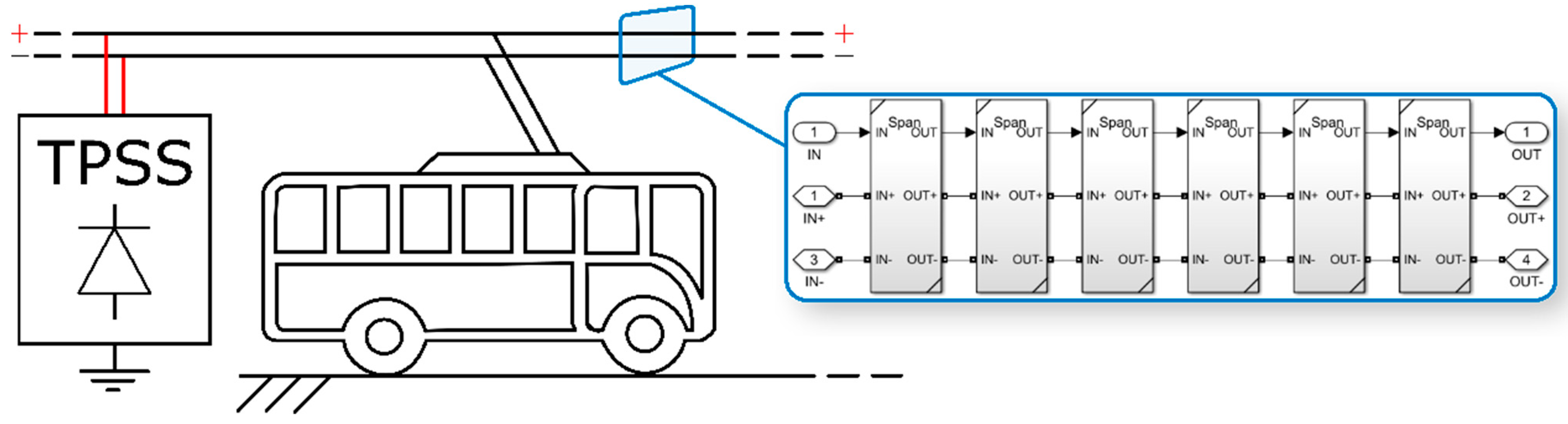
4. Proposed Multi-Vehicle Motion-Based Model of the Catenary in Simulink

In this work, multi-vehicle motion-based modeling is intended to simulate a trolleybus network’s behavior as a function of the variation in vehicle position over time, also giving flexibility in choosing the number of vehicles. To such an end, a thorough study of the catenary system has proven to be essential, while detailed analysis of electrical substations, as well as the vehicle traction system, is beyond the scope of this paper. Indeed, each TPSS is represented with the Thevenin equivalent circuit, and as explained in the next paragraphs, a controlled current generator is designated for modeling the trolleybuses. A similar approach was adopted in [7,9,11,12] for rail transport systems.

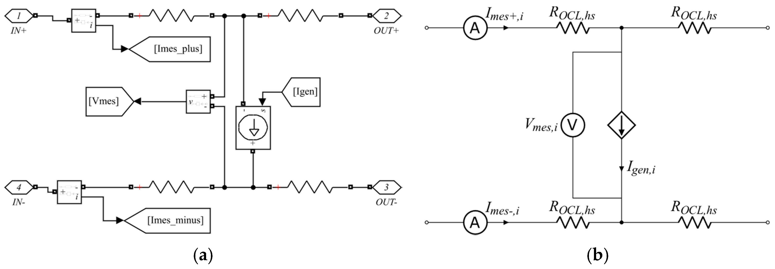
4.1. Modular Catenary Modeling

The idea behind the proposed Simulink model of the OCL is to represent the motion of the trolleybus. In this respect, the method devised in the present work concerns the introduction of subsystem reference (SR) blocks in Simulink [24]. In this way, one is allowed to save the contents of a subsystem in a separate file and reference them by using an SR block. One can create multiple instances referencing the same subsystem base block. When one edits any instance of a referenced subsystem, the changes are saved in the separate file in which the subsystem is stored, and all the referenced instances of that file are synchronized. By connecting more referenced subsystems together, it is possible to extend such a modular catenary model to the desired length and morphology. Figure 5 displays an example of an OCL model. All relevant data propagate in series between the adjacent blocks, allowing the space distribution of the electrical parameters such as line voltages, currents, and temperatures, albeit with a certain degree of discretization. In any case, such an approach results in a greater accuracy if compared with the conventional design method verified up to now, based on the evaluation of the electrical parameters at the FS macro-level.

A referenced subsystem adapts itself to the context of the parent model, which in our case includes a 20-m span of the overhead bifilar line. With the length of a typical articulated trolleybus being approximately 18 m, the chosen span length appears to be a good candidate for the discretization of the vehicle’s position. However, span lengths like 11 m and 25 m might be more appropriate when the trolleybus assortment is mainly composed of rigid or bi-articulated vehicles, respectively. Anyway, the SR strategy is very flexible from this viewpoint, allowing for adjusting the span to the wanted length. The span circuit included in the parent model is represented in Figure 6. The catenary span is modeled with resistors and a controlled current source, which represents the trolleybus current absorption, and it is turned on only if the position of the trolleybus itself corresponds to that specific SR block. In other words, the position over time of the trolleybus constitutes the driving parameter of the generator, which thus acts as a time-varying current source independent from any internal quantity. A given time-variant profile is assigned to the trolleybus position and current, which are set as inputs to the catenary model. The negligibility of reactive circuit components has been confirmed in the literature [9,11,12,13,14,15].

The circuit structure is built with an “H” configuration, where half-span resistors (having a resistance R_hs) are arranged symmetrically with respect to the central current source [25]. The “H” configuration derives from the choice of preserving the symmetry of the system to be able to apply changes more easily when extending the system itself. Although the accuracy of the introduced model might appear to be a shortcoming when compared to the variable resistor-based approach, such a discrepancy is compensated for by virtue of the theoretical possibility of increasing the spatial resolution at will. Nevertheless, for the purpose of this manuscript, a spatial discretization of 20 m is deemed sufficiently accurate.

4.2. Electrical Parameter Evaluation

Let us refer to Figure 6. The span parent model allows the achievement of line current and voltage space distributions through the related sensors (Current Measurement and Voltage Measurement Simscape blocks), enabling the verification of acceptability of the voltage variations as well as the inspection of possible overloads, respectively. Moreover, it features subsystems for determining the evolution of the voltage sensed by a trolleybus in its motion (i.e., the behavior of the line voltage as a function of time at the span where the vehicle is located), as well as the temperature pattern along the catenary.

An appropriate Matlab function was created to define whether the trolleybus was traveling within a certain referenced subsystem, which is useful for ensuring the activation of the correct current generator. The logic adopted for switching on the ith generator, representative of the vehicle current absorption at the ith SR block, is based on the equation below:

$$I_{Gen}=M\times I_T=\left[\begin{array}{c}{I}_{Gen,1}\\ ⋮\\ I_{Gen,i}\\ ⋮\\ I_{Gen,n}\end{array}\right]=\left[\begin{array}{ccccc}{m}_{11}& \cdots & m_{1j}& \cdots & m_{1N}\\ ⋮& \ddots & ⋮& \ddots & ⋮\\ m_{i1}& \cdots & m_{ij}& \cdots & m_{iN}\\ ⋮& \ddots & ⋮& \ddots & ⋮\\ m_{n1}& \cdots & k_{nj}& \cdots & m_{nN}\end{array}\right]\left[\begin{array}{c}{I}_{T,1}\\ ⋮\\ I_{T,J}\\ ⋮\\ I_{T,N}\end{array}\right],$$

(25)

where I_Gen is a column vector including the currents supplied by the generators between the positive and negative OCL poles inside each referenced subsystem, n is the number of SR blocks, N represents the number of vehicles considered, M is a sparse matrix whose only elements m_ij (with i = 1, …, n and j = 1, …, N), being equal to one, exist by virtue of the matching of the trolleybus positions and the referenced subsystems, and I_T is a column vector containing all the trolleybus currents set as inputs to the model. The current delivered by the generic ith generator within the ith SR block is defined as follows:

$$I_{Gen,i}={\displaystyle \sum }_{j=1}^N{m}_{ij}{I}_{T,j}.$$

(26)

Equation (26) agrees with the following conditions:

$$\{\begin{array}{c}{m}_{ij}=0, T_j\notin SR{B}_i \\ m_{ij}=1, T_j\in SR{B}_i\end{array}.$$

(27)

The results expressed by Equations (25) and (26) are obtained based on the hypothesis displayed in Equation (27). If the jth trolleybus (T_j) is inside the ith SR block (SRB_i), then the element m_ij equals one, and the current drawn by T_j (I_T,j) is assigned to I_Gen,i; otherwise, m_ij equals zero.

4.2.1. Voltage at the Trolleybus Location

The evaluation of the voltage to which the vehicle is subjected is deemed important for analyzing the OCL morphology. Hence, another Matlab function was built which still resorted to the M matrix. The logic behind this function is to assign the OCL voltage V_OCL,i at the ith SR block (i.e., the voltage V_mes,i measured by the ith voltmeter depicted in Figure 6) to the line voltage V_T,j at the location of the jth trolleybus, provided that the jth vehicle is within the ith SR block itself. The voltages seen by the trolleybuses are collected in a vector computed as follows:

$$V_T=M^{\mathrm{T}}\times V_{OCL}=\left[\begin{array}{c}{V}_{T,0}\\ ⋮\\ V_{T,J}\\ ⋮\\ V_{T,N}\end{array}\right]=\left[\begin{array}{ccccc}{m}_{11}& \cdots & m_{1i}& \cdots & m_{1n}\\ ⋮& \ddots & ⋮& \ddots & ⋮\\ m_{j1}& \cdots & m_{ji}& \cdots & m_{jn}\\ ⋮& \ddots & ⋮& \ddots & ⋮\\ m_{N1}& \cdots & m_{Ni}& \cdots & m_{Nn}\end{array}\right]\left[\begin{array}{c}{V}_{OCL,1}\\ ⋮\\ V_{OCL,i}\\ ⋮\\ V_{OCL,n}\end{array}\right],$$

(28)

The voltage sensed by the generic jth trolleybus (T_j) can be expressed as

$$V_{T,j}={\displaystyle \sum }_{i=1}^n{m}_{ji}{V}_{OCL,i}.$$

(29)

Equation (29) also fulfils the conditions listed in Equation (27).

As one may notice, the time dependence of the variables is not explicit here for the sake of compactness. However, since each trolleybus moves through different SR blocks, m_ij and m_ji change over time, and hence, the position of the respective switched-on generator varies temporally, as well as the V_OCL,i value assumed by the voltage V_T,j seen by the jth vehicle.

4.2.2. OCL Temperature

As for line overheat monitoring, with the aim of performing a reasonable comparison with the conventional approach, the OCL positive-pole steady state temperature at the ith SR block is calculated with Equation (4), which is adjusted accordingly:

$${\theta }_{OCL,ss,i}=C{\left(\frac{I_{OCL,i}}{S_{OCL}}\right)}^2+{\theta }_{OCL,0},$$

(30)

where I_OCL,i is the OCL positive-pole current at the ith SR block (i.e., the current I_mes+,i measured by the ith upper ammeter displayed in Figure 6).

5. Case Study of Feeding Sections in Bologna and Discussion of Results

The present section shows the application of the MVMB model to one of Bologna’s trolleybus routes inside a specific FS in Simulink environment. As the conventional design approach was actually adopted for the present trolleybus infrastructure, the corresponding outcomes were taken as the basis of comparison for verifying the simulation results. Two FSs, shown in Figure 7, were thoroughly analyzed by virtue of their peculiarities:

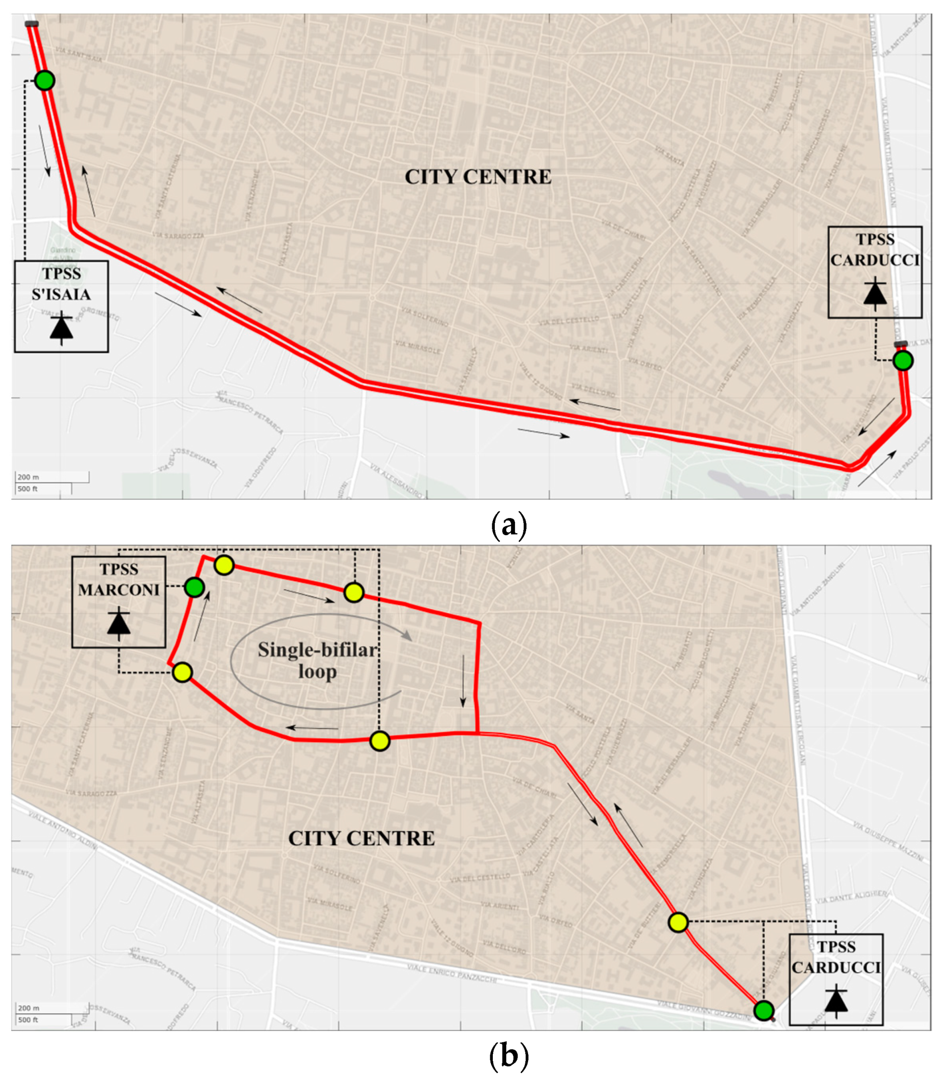
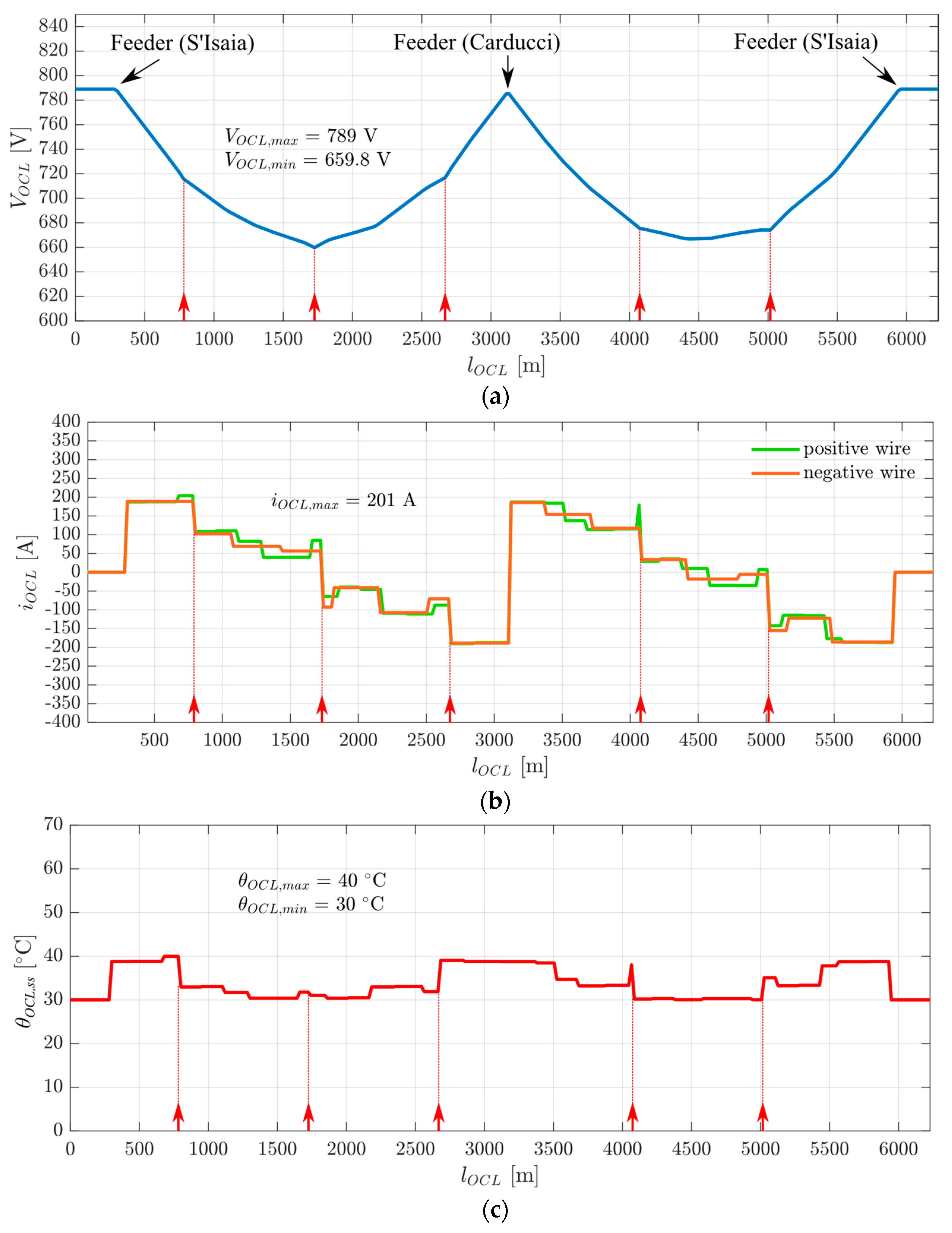
• FS “Sant’Isaia-Carducci” (FS 1): a bilaterally supplied FS (two feeding TPSSs (i.e., TPSS “Sant’Isaia” and TPSS “Carducci”) from which the FS designation was derived) with a basic topology (Figure 7a) (i.e., there exists an approximate symmetry of the double-bifilar line between the supply points). Rounded to the nearest multiple of 20 (i.e., the assumed span length in meters), the total bifilar length was 6240 m;
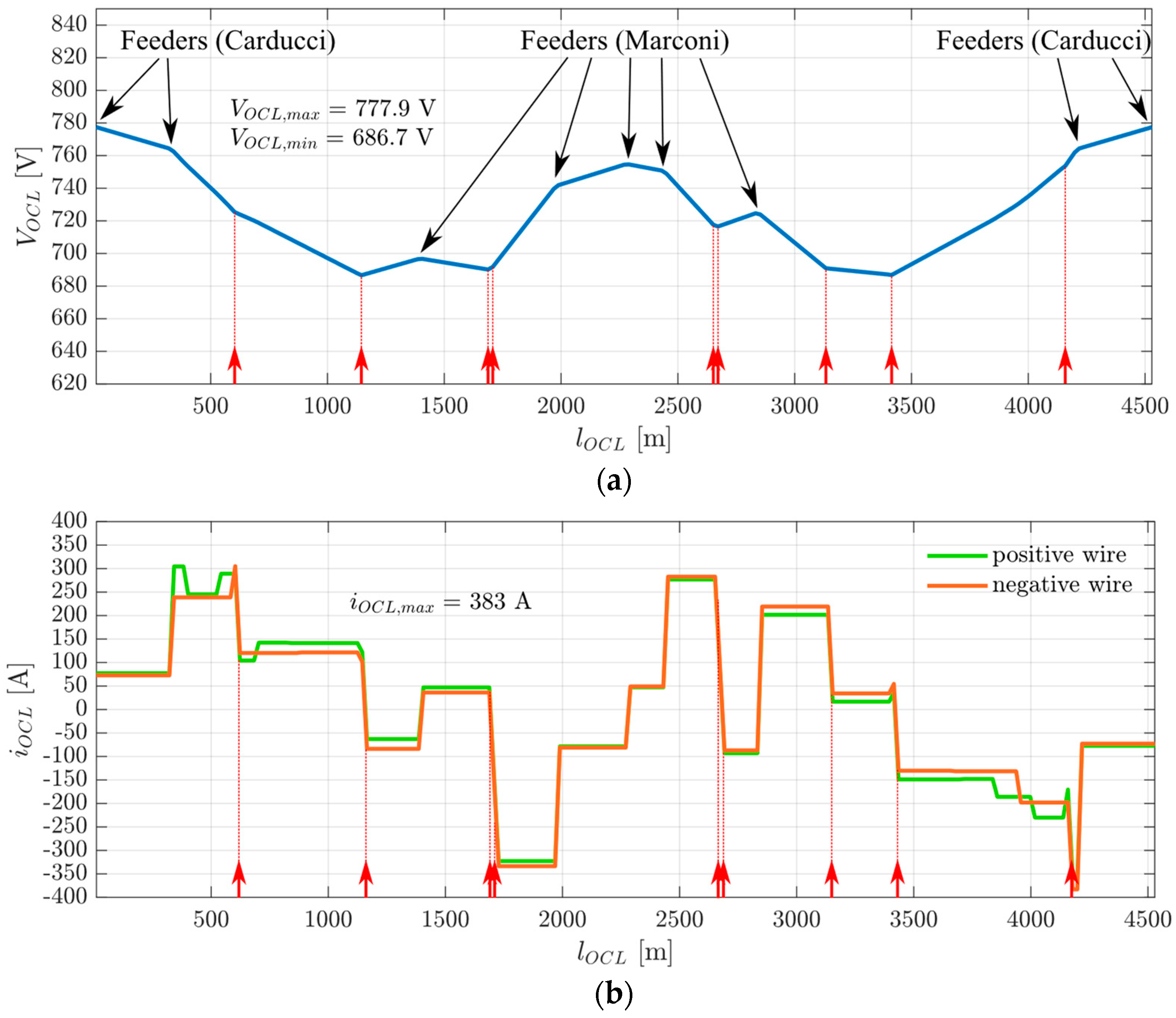
• FS “Marconi-Carducci” (FS 2): a bilaterally supplied FS with a complex structure (Figure 7b) due to the simultaneous presence of a double-bifilar line (towards TPSS “Carducci”) and a single two-wire loop (in the direction of TPSS “Marconi”), as well as the power support via several reinforcing feeders. Assuming the approximation made in the case above was valid, the total bifilar length was 4540 m.

Among the elements constituting the electrical infrastructure, particular emphasis was placed on the actual length and position of line feeders, reinforcing feeders, and equipotential bonding, with reference to the OCL path within the FS analyzed. While real data on conductors (made of copper) were provided by Trasporto Passeggeri Emilia-Romagna (TPER) S.p.A. and thus collected in

Table 2. Characteristics of the system conductors.

Label	Description	Parameters
ROCL,hs	OCL half-span (10 m) pole resistance	2.475 (mΩ)
SOCL	OCL nominal cross-section	100 (mm2)
C	OCL heat constant	2.5 (°C mm4/A2)
τth	OCL thermal time constant	600 (s)
θOCL,0	OCL initial temperature	30 (°C)

, Google Street View was exploited to determine the corresponding spatial coordinates [26]. It is worth emphasizing that the electrical resistance of one pole of the bifilar line was determined while considering a reference temperature of 75 °C (35 °C ambient temperature, plus 15 °C overtemperature due to solar radiation plus 25 °C due to the Joule effect) and a wear factor of 0.85 (attainable after 40 years of operation).

As mentioned in Section 4, TPSSs are modeled through the Thevenin equivalent circuit with a diode in series, which is a reasonable assumption for emulating 12-pulse rectifiers typically feeding transport systems relying on electric traction. Referring to this case study, we considered an open-circuit voltage V_th at the substation terminals of 830 V DC (hypothesizing 615 V on the AC side of the rectifier) and an equivalent series resistance of 68 mΩ in steady state conditions [27]. Based on the knowledge gained on Bologna’s trolleybus infrastructure, each TPSS is supposed to be grounded through a 0.5 Ω resistor.

For each FS considered here, two types of simulations were performed with different objectives, in any case, assuming that the trolleybus positions varied linearly over time.

The first simulation type served for a better understanding of the OCL morphology, being useful for proving the reasonableness of the MVMB model. For the sake of clearness, just one in-motion trolleybus was included in the FS, and the line voltage at its location was displayed.

As for the second simulation type, the MVMB model was set to reproduce the onerous operating conditions characterizing the conventional method with the aim of performing a reliable comparison between the results of the two approaches. Hence, the same number of trolleybuses considered in the conventional approach was introduced in the model, referring to the peak traffic hours. In this scenario, FS 1 and FS 2 included five and nine vehicles, respectively. For such a simulation type, the line voltage, current, and temperature were shown all over the FS at a significant time instance in which the trolleybuses were scattered with a certain criterion, as explained in the next paragraphs. Afterwards, with the purpose of verifying the simulation results, they were juxtaposed to the outcomes of the conventional method. To perform a proper comparison, the following considerations needed to be borne in mind both when setting the inputs and interpreting the simulation results:

• When analyzing the line current and temperature distributions, the total average current I_M in the FS was set as the overall load absorption (refer to Section 2.1) (i.e., for the sake of simplicity, each current source modeling the trolleybus drew (when due) a constant current I_T,j = I_M/N);
• Because of the structure of the conventional approach, we knew that it provided only one current and one temperature value for each FS, which both related to a worst-case scenario. Therefore, for the purpose of comparison, it was sensible to pick the maximum line current and temperature that the simulation gave along the whole FS;
• Similar to what has been emphasized about the current and temperature, the line voltage profile was evaluated by imposing the total starting current I_S in the FS as whole load absorption (see Section 2.2). Each vehicle thus drew a constant current I_T,j = I_S/N;
• The maximum voltage drop along the catenary section belonging to a certain FS was given by the difference between the maximum and the minimum voltage value.

5.1. Feeding Section “Sant’Isaia-Carducci”

Table 3. Feeding cables resistance per unit length of FS 1.

Label	Description	Parameters
rF,1S	TPSS “S’Isaia” feeder pole resistance per unit length	0.0250 mΩ/m
rF,1C	TPSS “Carducci” feeder pole resistance per unit length	0.0250 mΩ/m

collects the resistive parameters of the FS 1 feeding wiring harness.

5.1.1. First Simulation Type: OCL Morphology Analysis of FS 1

The graph in Figure 8 displays the catenary voltage trend that the only vehicle sensed while traveling within FS 1 as a function of its linearly time-varying position l_OCL (i.e., position along the single bifilar line to which the trolleybus was connected). The following remarks are provided:

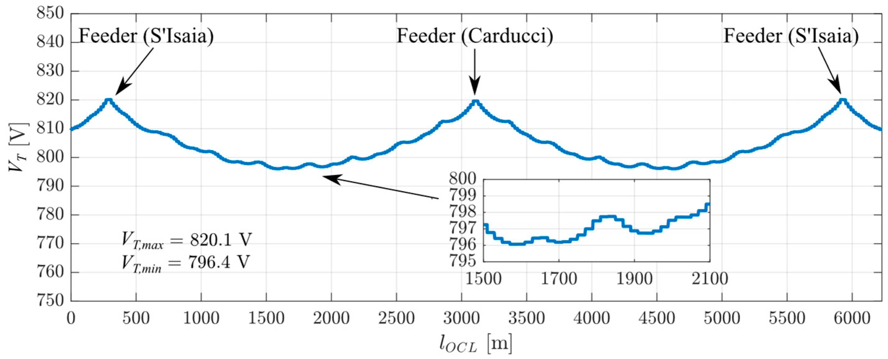
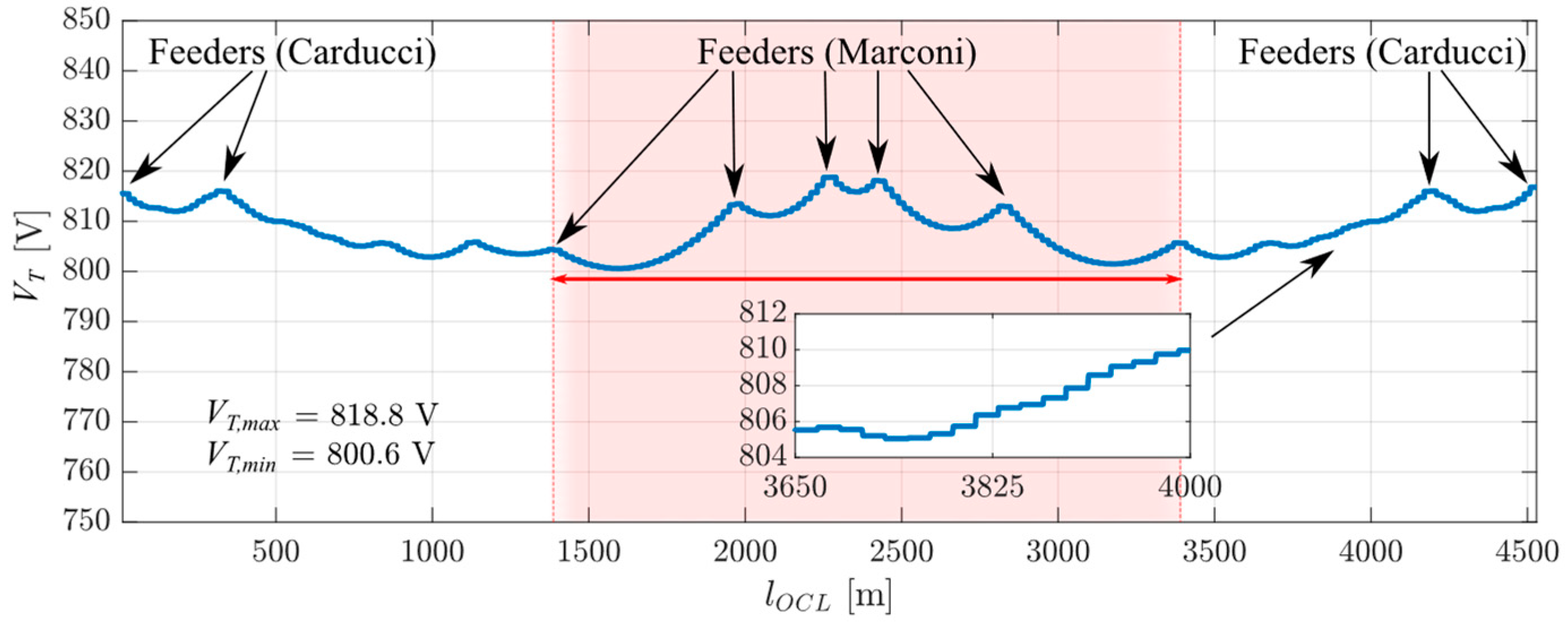
• A detail of the voltage trend emphasizes the 20-m spatial discretization;
• The horizontal axis coordinates of the voltage peaks correspond to the positions of the line feeders leaving from the TPSSs, as it should be. One may observe how the S’Isaia’s feeder connection point with the catenary was not in the exact extremity of the FS but slightly displaced towards the center;
• The voltage V_T is characterized by a undulatory behavior, owing to the presence of the equipotential bonding system set across the double-bifilar line. The slight increase in voltage in correspondence of such equipotential connections is attributable to the reduction in the catenary electrical resistance. Moreover, the effect of the double-bifilar OCL was that the trolleybus movement along one of the bifilar lines affected the current distribution in its counterpart, and hence a sort of symmetry in the undulatory phenomenon exists between the left and right halves of the plot.

5.1.2. Second Simulation Type: Method Comparison for FS 1

The present case included an attempt of evenly distributing the trolleybuses in the model to reproduce the conventional approach setting (see Section 2.2). Five vehicles were introduced to represent the busiest operating hours. By virtue of its structure, FS 1 got close to respecting hypothesis 1 in Section 2.1. The simulation results are plotted in Figure 9, which depicts the behavior along the catenary of the voltage between the positive and negative OCL poles, the current flowing in both poles, and the steady state temperature of the positive pole.

From the graphs in Figure 9, the data in question are extracted and collected in

Table 4. Results and techniques comparison for FS 1.

Label	Description	Conventional Method Parameters	MVMB Model Parameters
VOCL,max	OCL maximum voltage	750 V	789 V
VOCL,min	OCL minimum voltage	613 V	659.8 V
ΔVOCL	OCL voltage variation (VOCL,max − VOCL,min)	137 V	129.2 V
ΔVtot	Total voltage variation (Vth − VOCL,min)	137 V	170.8 V
IOCL	OCL positive-pole maximum current	187.5 A	201 A
θOCL,ss	OCL positive-pole maximum steady state temperature	39 °C	40 °C

, where the numerical results of the conventional method are also introduced. The red arrows indicate the vehicle positions.

All the results complied with the aforementioned standards [3,16] (i.e., V_OCL,min > 500 V, I_OCL < 451 A, and θ_OCL,ss < 80 °C). Since the conventional method disregarded the voltage drop for the feeders and rectifier (41 V), the MVMB model resulted in a noticeably higher total voltage variation. On the other hand, the small mismatch (7.8 V) for the OCL voltage variation between the two approaches was attributable to the TPSS “S’Isaia” feeder, which was connected about 300 m (refer to Figure 7a) after the beginning of the FS, leading to a virtually shorter OCL stretch length. The latter phenomenon is apparent in Figure 9, specifically in the first and last 300 m of the OCL section, where the null value of the current absorption (see Figure 9b) due to the absence of vehicles in that time instant did not produce any additional voltage drop or overtemperature. As for the current, the result obtained with the simulation was reasonably higher, since our Simulink model did not present the ideal double-bifilar line described in hypothesis 2 in Section 2.1. Indeed, it was not possible to achieve the perfect halving of the contact line current at any position that would occur in the case of OCLs, ideally in parallel. As one may see, the results of the two methods did not differ markedly. This means that the conventional method assumption of symmetry of the FS between the TPSS feeders could be adopted.

5.2. Feeding Section “Marconi-Carducci”

Table 5. Feeding cable resistance per unit length of FS 2.

Label	Description	Parameters
rF,2M	TPSS “Marconi” feeder pole resistance per unit length	0.0188 mΩ/m
rRF1,2M	TPSS “Marconi” reinforcing feeder 1 pole resistance per unit length	0.0601 mΩ/m
rRF2,2M	TPSS “Marconi” reinforcing feeder 2 pole resistance per unit length	0.2338 mΩ/m
rF,2C	TPSS “Carducci” feeder pole resistance per unit length	0.0150 mΩ/m
rRF,2C	TPSS “Carducci” reinforcing feeder pole resistance per unit length	0.0375 mΩ/m

gathers the resistive parameters of the FS 2 feeding cable system.

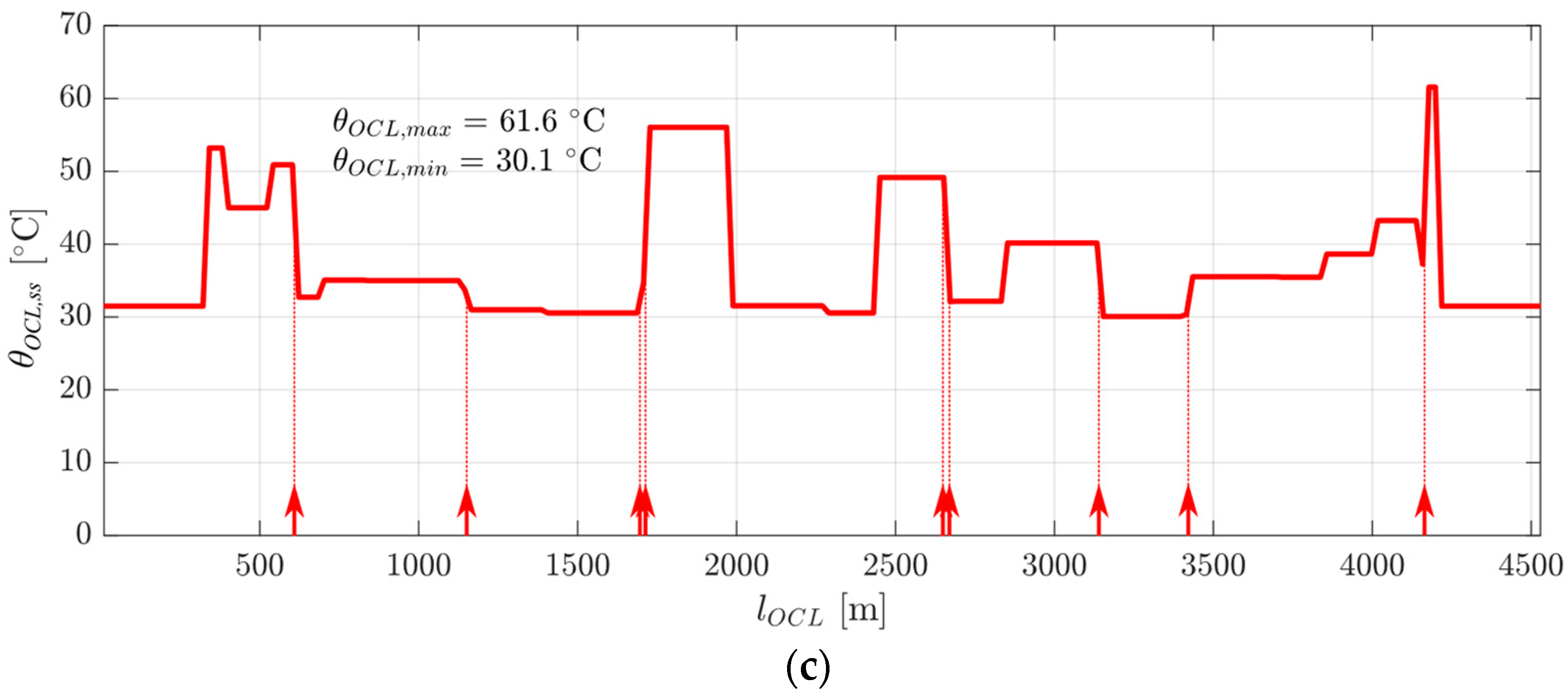
5.2.1. First Simulation Type: OCL Morphology Analysis of FS 2

Similar to FS 1, the graph in Figure 10 depicts the catenary voltage trend the sole trolleybus was subjected to while moving inside FS 2 at a constant speed. The following points may be added to the considerations made for FS 1, accounting for the greater complexity of the OCL topology (refer to Figure 7b):

• The voltage V_T was characterized by an undulatory behavior towards the TPSS “Carducci” at the plot extremity, owing to the presence of the equipotential bonding system set across the double-bifilar line. A symmetry in the undulatory phenomenon existed between the left and right plot extremities;
• The single two-wire ring presence was marked by the larger valleys belonging to the line section highlighted in red. Within these areas, no voltage equalizers were found.

5.2.2. Second Simulation Type: Method Comparison for FS 2

Due to the higher intricacy of FS 2′s structure, it became unfeasible to equally space the trolleybuses from the electrical viewpoint to replicate the conditions of the conventional approach. To simulate a possible worst-case scenario for the sake of comparison with the conventional method, nine vehicles (assuming peak-hour traffic) were arranged so that they were queued or on two different bifilar lines but at the same voltage equalizer. Following the same procedure as the previous case (see Section 5.1.2), the simulation results are plotted in Figure 11 below.

Table 6. Results and techniques comparison for FS 2.

Label	Description	Conventional Method Parameters	MVMB Model Parameters
VOCL,max	OCL maximum voltage	750 V	777.9 V
VOCL,min	OCL minimum voltage	603 V	686.7 V
ΔVOCL	OCL voltage variation (VOCL,max − VOCL,min)	147 V	91.2 V
ΔVtot	Total voltage variation (Vth − VOCL,min)	147 V	143.3 V
IOCL	OCL positive-pole maximum current	416 A	383 A
θOCL,ss	OCL positive-pole maximum steady state temperature	73 °C	61.6 °C

collects the numerical results of the conventional method as well as the simulation results obtained from Figure 11.

As can be noted, in this case, all the results also complied with the consulted standards (refer to Section 2), although the conventional approach gave a borderline outcome for the OCL pole current and temperature. This is explained by the assumed absence of reinforcing feeders (see Section 2.2). Even though the omission of reinforcing supply points stood as a precautionary consideration, the hypothesis of FS symmetry proper to the traditional approach led to underestimating the relative parameters in Table 6, which therefore are misleading. One may infer that for FSs of such a type, when dealing with the actual OCL morphology, the presence of reinforcing feeders is needed for meeting the standards.

6. Modeling Techniques Comparison

Table 7. Comparison of the catenary modeling techniques.

		Modeling Features
		Variable Number of Vehicles	Complex FS Morphology	User-Friendliness
Modeling methods	Conventional analytical approach	✓	✕	✕
	Train-sim	✓	✓	✕
	Variable resistor imitation	✕	✕	✓
	MVMB model	✓	✓	✓

clarifies whether the analyzed techniques for modeling the catenary achieved certain features, examined here one by one.

The conventional analytical approach permitted obtaining the line parameters at the FS’s macro-level through relatively simple mathematical expressions. Because of their strict dependence on the number of vehicles within the FS, the conventional method allowed easy changing of such a number. The Train-sim tool also had no difficulty in this direction, as it was only a matter of modifying the quantity of the electrical nodes via coding. By contrast, the Simulink-based catenary models found in the literature did not concede flexibility in varying the amount of vehicles. The number of vehicles defined how many variable resistor models would be used to simulate one FS, and it could not be assumed they were identical, as the distances between the different vehicles may have varied according to the traffic intensity and the specific speed profile of each. On the other hand, with the modular MVMB model owing to the SR blocks, it permitted simulating any trolleybus fleet by simply switching on the current sources in the corresponding vehicle positions.

As already discussed, most of the trolleybus system FSs are characterized by a greater morphology complexity if compared to railway ones. Within FSs of that typology, because of the simplifying hypotheses that delineate the conventional approach, it does not consider the presence of reinforcing feeders, the asymmetry of the TPSSs (see Section 1), the possible combination of single- and double-bifilar lines, the actual distribution of the equipotential bonding system, or the grounding system. Moreover, the FS topology intricacy grows with the introduction of stationary energy storage systems for supporting the trolleybus grid, as well as with the idea of using the grid itself for charging electric vehicles. Hence, the conventional method, which is already based on a maximalist scenario, appears to be excessively precautionary in the event of intricated FSs, leading to unreliable electrical parameters. Concerning the variable resistor-based catenary models developed in Simulink, the way they were built made us deduce that the displacement of the TPSS feeders and the addition of reinforcing feeders or voltage equalizers at any point on the OCL was unrealizable. As for the Train-sim simulator, on the other hand, the addition of supply points and equipotential bonding in this case was also just a matter of increasing the number of electrical nodes for the network calculations. The internal code exactly defined all the OCL branches forming the FS. Getting to the MVMB model, once again, thanks to the modularity property, any FS topology intricacy could be handled. This model could prove if the trolleybus network might work as a DC backbone for EV fast charging. To a first approximation, charging stations might be considered as current sources absorbing current from the OCLs, and hence its effects on the overall trolley grid may be studied. In addition, one could understand whether it is feasible to substitute the reinforcing feeders with other support middle-bay supplies in critical areas, such as stationary energy storage systems (e.g., backup batteries). In the case of voltage drops, such systems would act by providing power to the lines. Exploiting the SR blocks, our model is generalizable for any metropolitan trolleybus network (e.g., Kiev, Minsk, San Francisco, and so on), most of which operate at voltages lower than 750 V DC (typically 600 V DC), making the integration of stationary energy storage even more important for tackling the presumably higher voltage drops. Moreover, the backup batteries could manage the power flows to avoid overloads and lead to a better handling of traffic jam conditions.

Let us now focus on the user-friendliness of the studied methodologies. Regarding the conventional approach, although the respective equations may be implemented in electronic spreadsheets (e.g., Excel) or in diverse programming environments (e.g., Matlab) in a straightforward manner, one may realize the lack of intuitiveness of its use. Concerning the simulation tools, the man–machine interface in the Train-sim simulator is also not flexible, as Fortran is a programming language that mainly involves writing code. On the contrary, Simulink provides a graphical interface, and hence the structures of the catenary models and related parameters may be easily adjusted.

7. Conclusions

A novel multi-vehicle motion-based model of trolleybus traction catenary systems was proposed in this work. Thanks to the availability of subsystem reference blocks in the Simulink built-in libraries, the presented catenary model was characterized by modularity as a strong point, which made it proficient in managing different traffic conditions and in reproducing actual contact line structures. Such a feature generalized the model for any other dynamic conductive power transfer application, enabling the analysis of interconnected multimodal urban transportation systems together with the verification of the possibility of partial infrastructure sharing.

This paper has provided a critical review of the existing modeling techniques adoptable for contact-wire-based traction systems, demonstrating the reasonableness of the presented approach. The conventional design method in effect today, although straightforward and effective in the case of FSs with basic structures, becomes inevitably incompatible with the demand for the modernization of trolley networks. Despite the intuitiveness provided by the graphical interface of Simulink with respect to Fortran, the respective variable resistor-based models reviewed in this paper may not prove suitable for dealing with complex network morphologies or allowing the variability of the number of vehicles.

The MVMB model was tested for Bologna’s trolleybus network, and its consistency with the respective OCL morphology was shown graphically. By examining the distribution of the line voltage, current, and temperature along the catenary, the limitations of the conventional approach were delineated and demonstrated, especially concerning FSs with intricated structures. Indeed, the hypotheses that guide such an analytical method prove to be unenforceable for FSs of greater complexity, making this model obsolete despite the standard conformity of the achieved results.

To conclude, the proposed model could help with investigating next-future technological features for developing smart electric traction grids, such as stationary ESS and RES integration for IMC technology optimization, EV fast charging via catenary networks, and controlled bidirectional rectifier TPSSs for managing power flows and preventing system disruptions, all of which are aspects that allow catenary-powered transport systems to be included in the context of smart city evolution.

References

1. Breuer, J.L.; Samsun, R.C.; Stolten, D.; Peters, R. How to reduce the greenhoue gas emissions and air pollution caused by light and heavy duty vehicles with battery-electric, fuel cell-electric and catenary trucks. Environ. Int. 2021, 152, 106474. [Google Scholar] [CrossRef] [PubMed]
2. Ahmadi, M.; Jafari Kaleybar, H.; Brenna, M.; Castelli-Dezza, F.; Carmeli, M.S. Integration of Distributed Energy Resources and EV Fast-Charging Infrastructure in High-Speed Railway Systems. Electronics 2021, 10, 2555. [Google Scholar] [CrossRef]
3. CENELEC. EN 50119 Railways Applications-Fixed Installations-Electric Traction Overhead Contact Lines; CENELEC: Brussels, Belgium, 2020. [Google Scholar]
4. Perticaroli, F. Sistemi Elettrici per i Trasporti: Trazione Elettrica [Electrical Systems for Transportation: Electric Traction]; CEA: Milan, Italy, 2001. [Google Scholar]
5. Mayer, L. Impianti Ferroviari: Tecnica ed Esercizio [Railway Installations: Technique and Exercise]; Collegio ingegneri ferroviari italiani: Rome, Italy, 1989. [Google Scholar]
6. Capasso, A.; Lamedica, R.; Penna, C. Energy Regeneration In Transportation Systems—Methodologies For Power-Networks Simulation. In Control in Transportation Systems, Proceedings of the 4th IFAC/IFIP/IFORS Conference, Baden-Baden, Federal Republic of Germany, 20–22 April 1983; Elsevier: Amsterdam, The Netherlands; pp. 119–124.
7. Adinolfi, A.; Lamedica, R.; Modesto, C.; Prudenzi, A.; Vimercati, S. Experimental assessment of energy saving due to trains regenerative braking in an electrified subway line. IEEE Trans. Power Deliv. 1998, 13, 1536–1541. [Google Scholar] [CrossRef]
8. Lamedica, R.; Gatta, F.M.; Geri, A.; Sangiovanni, S.; Ruvio, A. A Software Validation for DC Electrified Transportation System: A Tram Line of Rome. In Proceedings of the 2018 IEEE International Conference on Environment and Electrical Engineering and 2018 IEEE Industrial and Commercial Power Systems Europe (EEEIC/I&CPS Europe), Palermo, Italy, 12–15 June 2018; pp. 1–6. [Google Scholar] [CrossRef]
9. Capasso, A.; Lamedica, R.; Ruvio, A.; Ceraolo, M.; Lutzemberger, G. Modelling and simulation of electric urban transportation systems with energy storage. In Proceedings of the 2016 IEEE 16th International Conference on Environment and Electrical Engineering (EEEIC), Florence, Italy, 7–10 June 2016; pp. 1–5. [Google Scholar] [CrossRef]
10. Capasso, A.; Ceraolo, M.; Lamedica, R.; Lutzemberger, G.; Ruvio, A. Modelling and simulation of tramway transportation systems. J. Adv. Transp. 2019, 2019, 4076865. [Google Scholar] [CrossRef] [Green Version]
11. Alnuman, H.; Gladwin, D.; Foster, M. Electrical modelling of a DC railway system with multiple trains. Energies 2018, 11, 3211. [Google Scholar] [CrossRef] [Green Version]
12. Mao, F.; Mao, Z.; Yu, K. The Modeling and Simulation of DC Traction Power Supply Network for Urban Rail Transit Based on Simulink. J. Phys. Conf. Ser. 2018, 1087, 042058. [Google Scholar] [CrossRef]
13. Sirmelis, U. Direct connection of SC battery to traction substation. In Proceedings of the 2015 56th International Scientific Conference on Power and Electrical Engineering of Riga Technical University (RTUCON), Riga, Latvia, 14 October 2015; pp. 1–5. [Google Scholar] [CrossRef]
14. Fan, F.; Stewart, B.G. Power Flow Simulation of DC Railway Power Supply Systems with Regenerative Braking. In Proceedings of the 2020 20th IEEE Mediterranean Electrotechnical Conference (MELECON), Palermo, Italy, 16–18 June 2020; pp. 87–92. [Google Scholar] [CrossRef]
15. Stana, G.; Brazis, V. Trolleybus motion simulation by dealing with overhead DC network energy transmission losses. In Proceedings of the 2017 18th International Scientific Conference on Electric Power Engineering (EPE), Kouty nad Desnou, Czech Republic, 3 July 2017; pp. 1–6. [Google Scholar] [CrossRef]
16. CENELEC. EN 50163 Railway Applications-Supply Voltages of Traction Systems; CENELEC: Brussels, Belgium, 2004. [Google Scholar]
17. Rusck, S. The simultaneous demand in distribution network supplying domestic consumers. ASEA J. 1956, 10, 59–61. [Google Scholar]
18. Dickert, J.; Schegner, P. Residential load models for network planning purposes. In Proceedings of the 2010 International Symposium on Modern Electric Power Systems (MEPS’10), Wroclaw, Poland, 20–22 September 2010; pp. 1–6. [Google Scholar]
19. Sun, M.; Djapic, P.; Aunedi, M.; Pudjianto, D.; Strbac, G. Benefits of smart control of hybrid heat pumps: An analysis of field trial data. Appl. Energy 2019, 247, 525–536. [Google Scholar] [CrossRef]
20. Du, W. Probabilistic analysis for capacity planning in Smart Grid at residential low voltage level by Monte-Carlo method. Procedia Eng. 2011, 23, 804–812. [Google Scholar] [CrossRef] [Green Version]
21. Vergnes, H.; Nijhuis, M.; Coster, E. Using Stochastic Modelling for Long-Term Network Planning of LV Distribution Grids At Dutch DNO. In Proceedings of the 25th International Conference and Exhibition on Electricity Distribution CIRED, Madrid, Spain, 3–6 June 2019. [Google Scholar]
22. Schick, C.; Klempp, N.; Hufendiek, K. Impact of network charge design in an energy system with large penetration of renewables and high prosumer shares. Energies 2021, 14, 6872. [Google Scholar] [CrossRef]
23. Fürst, K.; Chen, P.; Gu, I.Y.H.; Tong, L. Improved peak load estimation from single and multiple consumer categories. In Proceedings of the CIRED 2020 Berlin Workshop, Online Conference, 22–23 September 2020; pp. 178–181. [Google Scholar] [CrossRef]
24. MATLAB & Simulink. The MathWorks Inc. Subsystem Reference. Available online: https://www.mathworks.com/help/simulink/ug/referenced-subsystem-1.html (accessed on 5 September 2021).
25. Ruffo, R.; Cirimele, V.; Guglielmi, P.; Khalilian, M. A coupled mechanical-electrical simulator for the operational requirements estimation in a dynamic IPT system for electric vehicles. In Proceedings of the 2016 IEEE Wireless Power Transfer Conference (WPTC), Aveiro, Portugal, 5–6 May 2016; pp. 1–4. [Google Scholar] [CrossRef]
26. Google Maps (n.d.) Bologna, IT. Available online: http://shorturl.at/pvFHZ (accessed on 7 October 2021).
27. Baghramian, A.; Forsyth, A.J. Averaged-value models of twelve-pulse rectifiers for aerospace applications. In Proceedings of the Second International Conference on Power Electronics, Machines and Drives (PEMD), Edinburgh, UK, 31 March–2 April 2004; Volume 1, pp. 220–225. [Google Scholar] [CrossRef]
Figure 1. Coincidence factor as a function of the number of vehicles.
Electronics 11 00915 g001
Figure 2. Unilateral power supply with a uniformly distributed load.
Electronics 11 00915 g002
Figure 3. Voltage drop plus factor.
Electronics 11 00915 g003
Figure 4. Bilateral power supply with a uniformly distributed load.
Electronics 11 00915 g004
Figure 5. Catenary modeling with Subsystem Reference blocks.
Electronics 11 00915 g005
Figure 6. “H” configuration of the OCL span model, showing the Simulink representation (a) and circuit schematic drawing (b).
Electronics 11 00915 g006
Figure 7. Bologna’s FSs selected for the case study. The trolleybus routes (oriented by arrows) of the FS “S’Isaia-Carducci” (a) and FS “Marconi-Carducci” (b) are plotted together with TPSSs and supply points (connection points of line feeders with the OCL in green and of reinforcing feeders in yellow).
Electronics 11 00915 g007
Figure 8. OCL voltage sensed by the trolleybus traveling along FS 1.
Electronics 11 00915 g008
Figure 9. Distributions of OCL voltage (a), pole currents (b), and steady state temperature (c) along FS 1. Trolleybus positions are marked by red arrows.
Electronics 11 00915 g009
Figure 10. OCL voltage sensed by the trolleybus traveling along FS 2.
Electronics 11 00915 g010
Figure 11. Distributions of OCL voltage (a), pole currents (b), and steady state temperature (c) along FS 2. Trolleybus positions are marked by red arrows.
Electronics 11 00915 g011aElectronics 11 00915 g011b