Analysis of Electric Energy Consumption Profiles Using a Machine Learning Approach: A Paraguayan Case Study

Abstract

Correctly defining and grouping electrical feeders is of great importance for electrical system operators. In this paper, we compare two different clustering techniques, K-means and hierarchical agglomerative clustering, applied to real data from the east region of Paraguay. The raw data were pre-processed, resulting in four data sets, namely, (i) a weekly feeder demand, (ii) a monthly feeder demand, (iii) a statistical feature set extracted from the original data and (iv) a seasonal and daily consumption feature set obtained considering the characteristics of the Paraguayan load curve. Considering the four data sets, two clustering algorithms, two distance metrics and five linkage criteria a total of 36 models with the Silhouette, Davies–Bouldin and Calinski–Harabasz index scores was assessed. The K-means algorithms with the seasonal feature data sets showed the best performance considering the Silhouette, Calinski–Harabasz and Davies–Bouldin validation index scores with a configuration of six clusters.

1. Introduction

In electric distribution networks, the identification of electric load profiles is of great interest for electric energy distribution network planners and operators [1] (DNOs). The grouping distribution of feeders can be useful for tasks such as the simulation of the impact of new grid technologies, new tariffs, or network re-configurations [2]. Furthermore, the identification of a set of representative feeders allows the load distribution to be modeled avoiding an exhaustive simulation process on every feeder of the network.

To identify representative feeders, operators often use deterministic and aggregated load models [3]. This approach is straightforward to apply and clear to assess. However, it fails in the presence of uncertainties leading to suboptimal solutions. In order to integrate the uncertainties, probabilistic and optimization load modeling approaches have been applied [4]. Despite the improvement with respect to the aggregated model, they require detailed knowledge or assumptions at an appliance level [5]. To overcome this problem, the clustering approach finds the best model according to the data. In this approach, different electric characteristics are taken into consideration to generate the model [2]. In [6], a data-driven time series clustering method is proposed to provide meaningful and intuitive profiles to describe the behaviors of consumers at the local electrical grid level. Other important applications of electrical consumption clustering include the characterization of load curves in a real distribution system [7] and load profiling for tariff design and load forecasting or distribution planning [8].

The application of descriptive analyses to electric consumption data allows insights about electrical usage behaviour to be obtained. For example, in [9], a clustering analysis is applied for the determination of the optimal placement of distributed generation sources in electrical distribution systems. The results reveal that the feeders with peak demand in the early afternoon are more likely to be better candidates for distributed photovoltaic generation. Another interesting application is the demand-side management. In [10], the clustering analysis is helpful for identifying different consumption profiles and implementing demand-side response programs or specific incentives to modify consumer demand.

In this work, we address this problem by applying two clustering strategies on a data set containing electric consumption data generated in Paraguay and provided by the Paraguayan electric company. In particular, we applied K-means and hierarchical agglomerative clustering and analyzed the results. Moreover, since clustering techniques use a distance measure to establish the clusters, we evaluated two different measures, the Euclidean and the dynamic time warping (DTW) measures [11]. DTW was considered convenient since data are organized as time series.

The data corresponded to the eastern region of the country and were recorded from January 2017 to December 2020, with measurements recorded every hour and a half. It is important to remark that these data were obtained and made public as part of the same research protect that made this paper possible [12]. In order to be used, the raw data were processed to obtain the following four data sets applicable to the clustering analysis:

• Weekly time series data, where the consumption of each feeder was aggregated on a weekly basis;
• Monthly time series data, where the consumption of each feeder was aggregated on a monthly basis;
• Statistical data set—a set of statistical features was calculated from the raw data;
• Seasonal and daily load curve feature data set—a set of features based on the daily load curve and seasonal consumption variations was computed.

We can summarize the contributions of this work as follows:

• Analysis and comparison of the performance of different clustering algorithms using real electricity consumption data collected from a Paraguayan electricity provider.
• Study of the suitability of four different data processing strategies.
• Evaluation of the influence of distance metrics and linkage criteria for this particular case study.

The rest of the paper is organized as follows: In Section 2, related works are presented. Then, the raw data, data processing, clustering algorithms and related techniques are described in Section 3. Section 4 shows the algorithms results and, finally, in Section 5, the conclusions and future work are proposed.

2. Related Works

There is a growing concern to address energy-related problems such as electricity consumption, load and demand. Understanding different energy consumption patterns or measuring the environmental impact of energy production can help the adoption of new policies according to demand–response scenarios [13], as well as more sustainable energy policies [14]. In the literature, much attention has been given to electricity consumption prediction [15]. In [16], for example, Walket et al. applied several learning algorithms—boosted tree, random forest, support vector machine (SVM) and artificial neural networks—to predict commercial building electricity demands. Liu et al. [17] applied SVM to public buildings’ energy consumption from Wuhan (China). In this case, the energy consumption data were combined with climatic and time-cycle factors. Many other works using the supervised approach can be found [18,19,20].

Clustering, although to a lesser extent than said predictive methods, has also been studied in the literature. There are several relevant works in the field. For example, Diao et al. [21] used a clustering approach to identify and classify the behaviour of occupants analysing energy consumption outcomes and energy time use data. Pérez-Chacón et al. [22] applied this approach to extract the energy consumption pattern of smart cities in a big data context. The method proposed was tested using electricity consumption during the years 2011–2017 for eight buildings in a public university. Divina et al. [23] applied the biclustering approach to find anomalies in the energy consumption pattern of smart buildings from a Spanish university campus. In [24], Pinto-Roa et al. proposed to extend an evolutionary algorithm to the time-series approach to identify consumption user profiles.

Feature extraction is another interesting approach. It entails proposing new features from the original ones to enhance relevant information. In this context, disregarding temporal information results in the loss of time-related information and redundancy of features. In this context, Meng et al. [25] applied a discrete wavelet transform (DWT) to decompose the raw data. The DWT is not only capable of extracting the rising trend and periodic waves, but it can also distinguish stochastic behavior. Neural networks (NN) were used to predict periodic waves, which can simulate their increasing amplitude. For this work, in which electric energy consumption data from China were under analysis, the results suggest the competitiveness of the proposal for a forecasting purpose. In [26], Luo et al. developed an integrated artificial intelligence-based approach that was combined with an evolutionary algorithm to enhance an adaptive deep neural network model. The proposal was tested on hourly energy consumption data. Liang et al. [27] presented a hybrid model. Such model combined empirical mode decomposition, minimal redundancy, maximal relevance and general regression neural network with fruit fly optimization algorithm. This approach, called EMD-mRMR-FOA-GRNN, was validated using load data from the Chinese city of Langfang. Finally, a systematic time series feature extraction method called hierarchical time series feature extraction was proposed by Ouyanf et al. [28]. This model was used for supervised binary classification tasks and only used user registration information and daily energy consumption data to detect anomaly consumption users with an output of stealing probability. The performance of this proposal was tested using data from over 100,000 customers.

3. Materials and Methods

This section introduces the nature of the electric energy consumption data and provides the basic concepts of time series and feature-based clustering. The data used in this work, the characteristics calculated for the feature-based clustering approach and the basic notions of the clustering algorithms used are all described here.

Electric energy consumption data are usually represented as a time series through a discrete sequence of data points measured at equal time intervals.

Let $X={\left\{X_i\right\}}_{i=1}^N$ be a set of N univariate time series, where $X_i={\left\{x_{i,t}\right\}}_{t=1}^T$ is one of them and is characterized by T real values. Thus, the sample X can be represented through a matrix $H_{N\times T}$.

In the context of these particular data, each time series represents a sequence of sensor data collected over time. Therefore, the data can be viewed as an $N\times T$ energy consumption data matrix EM. EM is a real matrix, where each element $e_{it}$ represents the electric energy consumption of a feeder (expressed in kWh) as measured by sensor i at the hour t.

Another approach to represent the electric energy consumption is to calculate a set of features representing each electric consumption sequence instead of considering it as a time series [29]. The main advantages of this feature-based clustering method are: the ability to reduce the dimensionality of the original time series; the fact that it is less sensitive to missing values; and the fact that it can handle different lengths of time series [29]. The two feature data set representations implemented in this paper are described in Section 3.3.

3.1. Data

The data set used in this work contained 2,967,224 records of electric consumption measured in amperage from January 2017 to December 2020 (4 years) of 115 feeders distributed in 17 substations of the eastern region in Paraguay.

The data set, named “Electricity consumption and meteorological data of Alto Paraná, Paraguay”, is freely and publicly available at [12].

3.2. Data Preprocessing

A couple of transformations were applied to the data set to reduce the error in the results. The first step was normalizing the time stamp value. For example, 23:59:59 on a given day was converted to 00:00:00 of the next day. The elimination of negative and zero electric consumption records was applied. Since the collected data did not have a standard timing interval (records were saved every thirty minutes in some periods; in others every hour), the next step was the hourly frequency normalization. All records that did not match an o’clock time were removed from the set. Before the outlier detection and data imputation phase, feeders with less than $90\%$ of records were discarded. After all the preprocessing, 24 records per day from each feeder were expected over four years, i.e., feeders with less than 31.536 records were removed.

The result of these steps is a reduced data set made of 55 feeders distributed in 14 substations with at least $90\%$ of recorded hourly data during said four-year period.

With the reduced data set, outlier detection was performed using the algorithm proposed by Vallis et al. [30]. This algorithm requires a full data set. Thus, a linear interpolation to fill the gaps was needed before running it.

The Box–Cox transformation [31] was also used to stabilize the variance in the data, so that they remained stationary and obtained an additive time series as described by Chatfiel [32] and Hyndman et al. [33]. This resulted in $X^{*}$ as the Box–Cox transformation of X. Given the time series $X^{*}$, this algorithm implements the Seasonal and Trend decomposition using LOESS (STL) [34] to obtain the components of seasonality $S_{x^{*}}$, trend $T_{x^{*}}$ and remainder $R_{x^{*}}$, such that $X^{*}=S_{x^{*}}+T_{x^{*}}+R_{x^{*}}$. This decomposition method allows the seasonal component to be varied according to the nature of the series; simultaneously, it is robust to the presence of outliers.

After this, the remainder component was recalculated as $R_{x^{*}}=X^{*}-S_{x^{*}}-{\tilde{X}}^{*}$, where ${\tilde{X}}^{*}$ is the median of the data considering a non-overlapping moving window of two-week length as described in [30]. Then, the generalized extreme studentized deviate (ESD) test [35] was applied over the resulting remainder component using both median and median absolute deviation to detect outliers as described by Vallis et al. [30].

Finally, the inverse Box–Cox transformation was run. The outliers, as well as the interpolated values that were added at the beginning of this phase, were removed. The outliers quantity per feeder is shown in Figure 1.

After all outliers and unwanted records were discarded, the historical average data imputation technique [36] was applied to estimate each missing record $y_i$ as an average of $N_{\mathcal{H}}$ representative historical records $y_j,j\in \mathcal{H}$, where $\mid \mathcal{H}\mid =N_{\mathcal{H}}$. The set $\mathcal{H}$ included all historical records where the day of the week (DOW) is the same as the one on the missing record and within selected spans of it. The DOW guaranteed that historical means were calculated over records of the same days of the week and similar seasonal characteristics. The selected DOW span for this analysis was ±6 weeks. The resulting data set contained 1,848,947 records of 55 feeders distributed over 14 substations. Figure 2 shows the percentage and number of records per feeder.

3.3. Data Sets and Features

In this section, the making of the four data sets used is explained.

The first data set provided the weekly demand registered by the feeders. Calculations considered a Sunday-to-Saturday span, resulting in a time series of 207 records. Sunday was chosen because the time series of the feeders began on that day, on 1 January 2017. Thus, an equitable distribution of the days for each week was obtained from the start. However, some days were dropped, even in the middle of the time series, due to missing data and some weeks yielded data with less than seven days.

The second data set contained the monthly demand, with a time series of 48 records. As on the first data set, some months had fewer data than others due to discarded data. December 2020 was the month with the fewest observations, only 16 days.

The third data set was considered from the work performed by Rasanen et al. [29]. Seven statistical features were extracted from each of the feeders in a window of size equal to one calendar week $N_i$ throughout the entire time series, where $i=1,2,\dots ,207$ weeks. It should be noted that, although $N_i$ corresponds to one week, it presents different lengths due to missing values in certain weeks.

Therefore, the features used were: mean ($\mu$), standard deviation ($\sigma$), skewness ($\mathcal{S}$), kurtosis ($\mathcal{K}$), maximum Lyapunov exponent ($\lambda$), energy ($\mathcal{E}$) and periodicity ($\mathcal{P}$). The mean, calculated by Equation (1), indicates the central value of the analyzed data. In contrast, the standard deviation (Equation (2)) indicates a measure of the dispersion of the data.

$${\mu }_i=\frac{1}{N_i}\sum _{t=1}^{N_i}{x}_{i,t}$$

(1)

$${\sigma }_i=\sqrt{\frac{1}{N_i}\sum _{t=1}^{N_i}{(x_{i,t}-{\mu }_i)}^2}$$

(2)

Skewness (Equation (3)) is a measure that indicates the degree of asymmetry in the distribution of the demand data [37]. Kurtosis (Equation (4)) is related to the tails in the distribution. High Kurtosis indicates greater extremity of deviations [37].

$${\mathcal{S}}_i=\frac{1}{N_i{\left({\sigma }_i\right)}^3}\sum _{t=1}^{N_i}{(x_{i,t}-{\mu }_i)}^3$$

(3)

$${\mathcal{K}}_i=\frac{1}{N_i{\left({\sigma }_i\right)}^4}\sum _{t=1}^{N_i}{(x_{i,t}-{\mu }_i)}^4$$

(4)

Likewise, chaotic dynamical systems are common natural and artificial phenomena, including energy demand. The measured time series comes from the attractor of an unknown system with a certain ergodicity. In other words, it refers to a set of numerical values towards which the system evolves. This ergodicity contains the attractor information [38]. The maximum Lyapunov exponent (MLE) is the most used quantity measured on chaotic systems, as it describes the exponential divergence of nearby trajectories. For the case of a time series $x_i=(x_{i,1},x_{i,2},\dots ,x_{i,N_i})$, a $\mathsf{\nu }$-dimensional phase attractor with delay coordinates is considered, i.e., a point on the attractor is represented by $\{x_{i,t},x_{i,t+\tau },x_{i,t+2\tau },\dots ,x_{i,t+(\mathsf{\nu }-1)\tau }\}$, where $\tau$ describes the almost arbitrarily considered delay and $\mathsf{\nu }$ the embedding dimension. Then, a initial point $\{x_{i,t_0},x_{i,t_0+\tau },x_{i,t_0+2\tau },\dots ,x_{i,t_0+(\mathsf{\nu }-1)\tau }\}$ is chosen and the nearest neighbor to it is determined [39]. The initial separation between these two selected points is represented by the vector $\delta {\mathit{Z}}_0$. Therefore, the system diverges approximately at a rate given by $\delta {\mathit{Z}}_t={\mathrm{e}}^{\lambda (t\times \Delta t)}\delta {\mathit{Z}}_0$, where $\lambda$ is the maximum Lyapunov exponent and $\Delta t$ the sampling period. Hereof, $\lambda$ became more accurate when $t\to N_i$. Therefore, it was estimated as the mean rate of separation of the nearest neighbors across the samples. Thus, the MLE was expressed according to Equation (5).

$${\lambda }_i=\frac{1}{N_i\times \Delta t}ln\frac{\left|\delta {\mathit{Z}}_t\right|}{\left|\delta {\mathit{Z}}_0\right|}$$

(5)

The energy present was also considered and was obtained using the fast Fourier transform (FFT) [40]. For this purpose, the resulting Fourier transform sequence was comprised by ${\mathcal{X}}_i\left[\mathbb{k}\right]={\mathcal{X}}_i\left[1\right],{\mathcal{X}}_i\left[2\right],\dots ,{\mathcal{X}}_i\left[N_i\right]$. Given this, the energy calculation was performed by adding the squares of the magnitudes of the resultant components; then, it was divided by the length of the sequence ($N_i$) to normalize the calculated measurement (Equation (6)).

$${\mathcal{E}}_i=\frac{{\displaystyle \sum _{\mathbb{k}=1}^{N_i}}{\left|\mathcal{X}\left[\mathbb{k}\right]\right|}^2}{N_i}$$

(6)

Finally, another highly relevant measure to assimilate the behavior of the time series is periodicity. To obtain it, a periodogram was determined to estimate the power spectral density, which also uses the FFT as the basis of the calculation. This function indicates the distribution of the frequencies present in the signal given by the time series. Hereof, the most powerful frequency was selected and converted into an hourly period value via Equation (7).

$${\mathcal{P}}_i=\underset{\mathcal{T}}{argmax}{\mathcal{P}}_{xx,i}\left(\omega \right)$$

(7)

where ${\mathcal{P}}_{xx,i}\left(\omega \right)$ represents the power spectral density in the frequency domain $\omega$ and $\mathcal{T}$ the period converted to hours, in which the power is higher.

The fourth data set was built in order to capture seasonal and daily effects on the energy demand, as in Haben et al. [41]. Consequently, each day was divided into five relevant periods that characterized the behavior of daily demand as shown in Figure 3. It is important to note that these periods were defined considering the Paraguayan electricity demand curve. Therefore, they are different from the proposal presented in [41]. The intervals of the chosen time periods are detailed in

Table 1. Time periods for seasonal data set consideration.

Time Period	Interval
1	10:00 p.m.–04:00 a.m.
2	05:00 a.m.–09:00 a.m.
3	10:00 a.m.–01:00 p.m.
4	02:00 p.m.–05:00 p.m.
5	06:00 p.m.–09:00 p.m.

.

The features to be used were defined, taking into consideration such periods. For a specific feeder and each period $i=1,2,3,4,5$ over the entire time series, $P_i$ was represented as the mean electricity demand with ${\sigma }_p$ corresponding to its standard deviation. Meanwhile, $\widehat{P}$ was considered as the mean daily demand over the complete time series. In each period, the mean demands corresponding to the summer and winter seasons, $P_i^S$ and $P_i^W$, respectively, were also computed. Similarly, the mean demands on weekdays and weekends were considered in each period of the entire time series. They were noted as $P_i^{WD}$ and $P_i^{WE}$, respectively. As a result, the following eight features were extracted:

• Features from 1 to 5: The relative average power in each time period over the entire time series given by

  $$P_i^R=\frac{P_i}{\widehat{P}}\mathrm{for}i=1,\dots ,5$$

  (8)
• Feature 6: Mean relative standard deviation over the entire time series given by

  $$\widehat{\sigma }=\frac{1}{5}\sum _{i=1}^5\frac{{\sigma }_i}{P_i}$$

  (9)
• Feature 7: A seasonal score given by

  $$\mathcal{S}=\sum _{i=1}^5\frac{|P_i^W-P_i^S|}{P_i}$$

  (10)
• Feature 8: A weekend vs. weekday difference score given by

  $$\mathcal{W}=\sum _{i=1}^5\frac{|P_i^{WD}-P_i^{WE}|}{P_i}$$

  (11)

It is important to mention that, for each data set obtained, the values of the preprocessed time series were scaled within a $[0,1]$ range for each feeder, through the transformation $x_{scaled}=\frac{x-x_{min}}{x_{max}-x_{min}}$, since, otherwise, the clustering process would have been carried out as a function of the mean daily demand [42]. Finally, the conformed data sets are represented in Figure 4.

3.4. Distance Measurements

The work aims to find similarities in feeder consumption. Thus, it was essential to determine appropriate distance measures. Since one of the strategies was based on feature extraction, the use of Euclidean distance was reasonable. However, when considering the strategy based on patterns present in the consumption time series, the distance measure based on dynamic time warping (DTW) proved to be a better choice [43], although the Euclidean distance showed some promising results that should be considered for experimentation [7].

Therefore, for the time series approach, the definition of the Euclidean distance is such that, given two time series $x=(x_1,x_2,\dots ,x_N)$ and $y=(y_1,y_2,\dots ,y_N)$ of lengths N, is represented as

$$d_e(x,y)=\sqrt{\sum _{i=1}^N{\parallel x_i-y_i\parallel }^2}$$

(12)

In the case of feature extraction, x and y correspond to the arrangement of the considered features.

On the other hand, the DTW algorithm presents an efficient method that minimizes shifting and distortion effects. It includes a transformation that allows similar shapes with different phases between time series to be detected [44]. Given the time series $x=(x_1,x_2,\dots ,x_N)$ and $y=(y_1,y_2,\dots ,y_N)$ of lengths N, a cost matrix is created with objects that correspond to the all pairwise distance between the x and y components, such that M: $m_{i,j}=\parallel x_i-y_j\parallel$ for $i,j\in [1,N]$. From here, the optimal warping path $wp=(p_1,p_2,\dots ,p_L)$ is determined, where $p_{\ell }=(i_{\ell },j_{\ell })$ represents the pair of indices of the selected components in the matrix M. The value of L corresponding to the length of $wp$ is such that $N\le L<2\times N$. For the determination of wp, there are three conditions to be followed. The first one corresponds to the boundary condition, in which $p_1=(1,1)$ and $p_L=(N,N)$; thus, it is ensured that such a path starts at the beginning of both series and closes at the end. The second refers to the monotonicity condition, where it is fulfilled that $i_{\ell -1}\le i_{\ell }$ and $j_{\ell -1}\le j_{\ell }$, in order to preserve the time-ordering of points. The third condition is known as the step size condition, whose criterion limits the warping path of the long jumps while aligning the series. This last condition is formulated as $p_{\ell }-p_{\ell -1}\in \{(1,1),(1,0),(0,1)\}$. Then, $wp$ is composed in such a way that the cost function $m_{wp}(x,y)={\sum }_{\ell =1}^L{m}_{i_{\ell },j_{\ell }}$ is minimized. Finally, the DTW distance is expressed as

$$d_{DTW}(x,y)=m_{wp}(x,y)$$

(13)

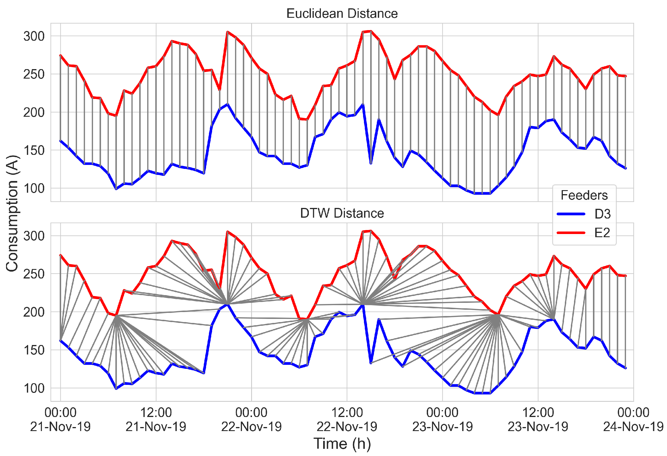
Figure 5 shows the difference between the components considered for the calculation of the distance between the D3 and E2 feeders, both Euclidean and DTW. The latter shows that the pairs of components considered were not necessarily located in the same temporal location.

3.5. Clustering Techniques

In machine learning, clustering refers to the process of grouping a sample of objects according to a similarity measure. Classically, clustering is defined as follows: Let $\mathcal{O}$ be a set of $n_o$ objects described by d features ${\mathit{⨏}}_j$, $j=1,2,\dots ,d$, so that $o_{ij}$ denotes the value of the feature ${\mathit{⨏}}_j$ for the object $o_i$.

Clustering aims to group the $n_o$ objects into K clusters $C_1,C_2,\dots ,C_K$ so that objects in the same cluster are more similar than those in other clusters.

The clustering algorithms used in this work are K-means [45] and hierarchical clustering [46]. The following section describes both strategies.

3.5.1. K-Means

The K-means algorithm is one of the simplest and most widely used clustering techniques. It determines cluster centroids belonging to a data set, according to a K value representing the number of clusters in which they are to be partitioned. In particular, the algorithm repeatedly performs two steps for this purpose. First, it assigns the closest centroid ($c_k$) to each data in order to minimize the sum of squared distance as expressed by Equation (14); then, it recalculates the centroids based on the mean of the data that were assigned to it, until it finds no variation or reaches a predefined number of iterations [47].

$$E=\sum _{k=1}^K\sum _{o\in C_k}{\parallel o-c_k\parallel }^2$$

(14)

It is worth noticing that the initialization of the centroids can be carried out randomly. Nevertheless, for this work, the Kmeans++ optimization method was used, thus selecting the starting points with a probability weighted by the distance from the previously chosen initial centroids [48]. In addition, it should be noted that, when K-means was applied on the time series data with the DTW distance measurement, the centroids were calculated using the DTW barycenter averaging (DBA) algorithm [49].

3.5.2. Hierarchical Clustering

Hierarchical clustering allows the construction of a hierarchy structure or linkage between the clusters formed, which can be either agglomerative or divisive. In the agglomerative method, each object is initially considered as a group. Then, the groups are iteratively combined to form an ascending hierarchy of groups until a single root group is reached. In contrast, the divisive method considers the complete set of objects as a single cluster. Then, it iteratively splits the clusters to achieve a top-down hierarchy where each object represents a single cluster [47].

The final structure of the clusters obtained is called a tree or dendrogram. The process carried out to obtain the dendrogram requires determining the similarity between the objects with the use of a linkage criterion [50]. In this work, a focus on the agglomerative method was given, using the linkage criteria summarized in

Table 2. Proposed linkage criteria for use in the hierarchical algorithm.

Criterion	Formula	Description
Single	$D(C_i,C_j)=\underset{o\in C_i,o^{\prime }\in C_j}{min}d(o,o^{\prime })$	Determined by the distance of the nearest objects between clusters $C_i$ and $C_j$.
Complete	$D(C_i,C_j)=\underset{o\in C_i,o^{\prime }\in C_j}{max}d(o,o^{\prime })$	Determined by the distance of the farthest objects between clusters $C_i$ and $C_j$.
Average	$D(C_i,C_j)=\frac{1}{\left|C_i\right|}\frac{1}{\left|C_j\right|}{\displaystyle \sum _{o\in C_i}}{\displaystyle \sum _{o^{\prime }\in C_j}}d(o,o^{\prime })$	Determined by the average distance between the objects of clusters $C_i$ and $C_j$.
Centroid	$D(C_i,C_j)=d(c_i,c_j)$	Determined by the distance between the centroids $c_i$ and $c_j$ corresponding to clusters $C_i$ and $C_j$, respectively.
Ward	$D(C_i,C_j)={\displaystyle \sum _{o\in C_i\cup C_j}}d{(o,c_{i,j})}^2$	Determined by sum of the squares of the distance between all objects in cluster $C_i$ and $C_j$, and $c_{i,j}$, centroid of the new cluster merged from $C_i$ and $C_j$.

. The application is described given two clusters, $C_i$ and $C_j$.

This approach was been applied to time series data. For example, in [51], the hierarchical algorithm was applied using the DTW distance.

3.5.3. K-Spectral Centroid

K-spectral centroid [52] (K-SC) allows clusters to be found in the time series based on the distinctive temporal pattern of the time series. It is an iterative algorithm similar to the classical K-means clustering algorithm, but performs an efficient centroid calculation under a scale-invariant and shift-invariant distance metric.

Similar to K-means, K-SC alternates between two steps to minimize the sum of squared distances; however, the distance metric is not Euclidean, but is given by

$$d_{SC}(x,y)=\underset{\gamma ,q}{min}\frac{\parallel x-\gamma y_q\parallel }{\parallel x\parallel }$$

(15)

where x and y correspond to time series, $y_q$ corresponds to the time series shifted by q time units and $\gamma$ is a scaling coefficient to time series. This measure finds the optimal alignment and the scaling coefficient for matching the shapes of the two time series. As a result, it allows one to compute the cluster centroids more appropriately by better acquiring the temporal patterns of the data. Thus, this algorithm was applied to the weekly and monthly time series of electricity demand.

3.6. Cluster Validity Indices

Since the task of grouping objects that share similar characteristics belongs to the area of unsupervised methods, it is challenging, at first, to select the number of sets to be considered. For this purpose, several clustering validation indices provide a quantitative criterion about the number of clusters formed. In this work, the Silhouette, Davies–Bouldin and Calinski–Harabasz validation indices were considered. They have shown promising results in comparative studies [53] and also provide enough information to select the most optimal configuration.

The Silhouette index describes a measure of quality based on how similar an object is to those belonging to the same cluster (cohesion) in contrast to how dissimilar it is from those belonging to the nearest cluster (separation) [54]. This index is normalized within a $[-1,+1]$ range, where high values indicate a good conformation of the objects based on their similarities concerning the distinctions of the other clusters. In this case, the average of the Silhouette index scores for each component of a given cluster was considered. Since ${\alpha }_i$ represents the average distance of an i-th sample for the others in the same cluster and ${\beta }_i$ represents the average distance of the same sample with respect to those in the nearest cluster, the Silhouette index for a sample is represented by

$${\mathit{⟆}}_i=\frac{{\beta }_i-{\alpha }_i}{max({\alpha }_i,{\beta }_i)}$$

(16)

Therefore, the average score of the Silhouette index is given by

$$SIL=\frac{1}{N}\sum _{i=1}^N\mathit{⟆}i$$

(17)

where N corresponds to the total amount of samples.

The Davies–Bouldin validation index represents the average similarity between clusters [55]. In this case, the cohesion estimation is based on the average distance ${\delta }_i$ between the centroid of a considered cluster i and the objects that conform it. The separation is represented by the distance ${\mathcal{D}}_{ij}$ between the centroids of the cluster i and another cluster j. Thus,

$$R_{ij}=\frac{{\delta }_i+{\delta }_j}{{\mathcal{D}}_{ij}}$$

(18)

is maximized, where ${\delta }_j$ represents the cohesion estimation for cluster j. Therefore, the Davies–Bouldin index is represented by the expression

$$DB=\frac{1}{K}\sum _{i=1}^K\underset{i\ne j}{max}{R}_{ij}$$

(19)

where K indicates the number of clusters. The lowest score that can be obtained for this index is 0; values close to it indicate better clustering.

Finally, the Calinski–Harabasz validation index measures the ratio of the sum of the between-cluster dispersion and within-cluster dispersion for all clusters [56]. In this sense, dispersion is defined as the sum of the squared distances. Therefore, when considering a set of objects $\mathcal{O}$ of size $n_o$, which have been clustered in one of the K clusters, it is necessary to determine both the between-cluster dispersion matrix B and the within-cluster dispersion matrix W, expressed as

$$B=\sum _{i=1}^K{n}_i(c_i-c_o){(c_i-c_o)}^T$$

(20)

$$W=\sum _{i=1}^K\sum _{x\in C_i}(x-c_i){(x-c_i)}^T$$

(21)

where $C_i$ indicates the set of objects belonging to cluster i, $c_i$ the center of cluster i, $c_o$ the center of $\mathcal{O}$ and $n_i$ the number of objects in cluster i. Once this is carried out, the traces $tr\left(B\right)$ and $tr\left(W\right)$ corresponding to the matrices B and W, respectively, are considered. With them, the Calinski–Harabasz index is defined as

$$CH=\frac{tr\left(B\right)}{tr\left(W\right)}\times \frac{n_o-K}{K-1}$$

(22)

High scores indicate well separated and dense clusters, which is expected when the clustering algorithm is correctly applied.

3.7. Workflow

As shown in Figure 6, this work followed a rigorous process to determine the necessary tools for experimentation. The starting point was collecting available data from the studied feeders, followed by the corresponding preprocessing to correct the anomalies present. Once this stage was completed, four sets were generated based on the above description.

The description of the different models induced on each data set are presented in

Table 3. Description of the proposed models.

Data Set	Algorithm	Distance	Linkage Criterion	Conformed Model ID
Weekly time series	K-Means	Euclidean	-	week_k-means_euclid
		DTW	-	week_k-means_dtw
	Hierarchical	Euclidean	Single	week_hier_euclid_single
			Complete	week_hier_euclid_complete
			Average	week_hier_euclid_average
			Centroid	week_hier_euclid_centroid
			Ward	week_hier_euclid_ward
		DTW	Single	week_hier_dtw_single
			Complete	week_hier_dtw_complete
			Average	week_hier_dtw_average
			Centroid	week_hier_dtw_centroid
			Ward	week_hier_dtw_ward
	K-Spectral Centroid	-	-	week_k-sc
Monthly time series	K-Means	Euclidean	-	month_k-means_euclid
		DTW	-	month_k-means_dtw
	Hierarchical	Euclidean	Single	month_hier_euclid_single
			Complete	month_hier_euclid_complete
			Average	month_hier_euclid_average
			Centroid	month_hier_euclid_centroid
			Ward	month_hier_euclid_ward
		DTW	Single	month_hier_dtw_single
			Complete	month_hier_dtw_complete
			Average	month_hier_dtw_average
			Centroid	month_hier_dtw_centroid
			Ward	month_hier_dtw_ward
	K-Spectral Centroid	-	-	month_k-sc
Statistical Based	K-Means	Euclidean	-	stats_k-means
	Hierarchical	Euclidean	Single	stats_hier_single
			Complete	stats_hier_complete
			Average	stats_hier_average
			Centroid	stats_hier_centroid
			Ward	stats_hier_ward
Seasonal Based	K-Means	Euclidean	-	seas_k-means
	Hierarchical	Euclidean	Single	seas_hier_single
			Complete	seas_hier_complete
			Average	seas_hier_average
			Centroid	seas_hier_centroid
			Ward	seas_hier_ward

. It gives a better appreciation of the configurations to be taken into account. For each data set, both the K-means and hierarchical clustering algorithms were applied, considering the corresponding variation depending on the nature of the data. Thus, for data belonging to time series, the analyses were performed for Euclidean distance measurement and DTW. On feature-based data, the only distance applied was the Euclidean distance. Likewise, for the models where the hierarchical algorithm was applied, the linkage criteria set out in Table 2 were taken into account. Therefore, each model was assigned an identifier for further analyses based on the results.

After the learning process was completed for different cluster sets, the validation index scores were considered to determine the best performing model and the optimal number of these clusters. Finally, the results were plotted to visualize the characteristics possessed by the conformed clusters, as shown in the next section.

4. Results

This section presents the results obtained from the numerical experimentation carried out using the previously defined models. The objectives defined in this work are the following:

• Comparison of the different clustering techniques studied to identify the best models according to the cluster validity index measures.
• Analysis of the consumption data of the best model found.l.

For the comparison of the different models, the number of clusters was varied from two to ten. For each model, the Silhouette, Davies–Bouldin and Calinski–Harabasz index scores were calculated. However, only the Silhouette index was taken into account because of its data independence [54].

However, since the preliminary results based on the Silhouette score yielded the best configuration of only two clusters, which did not imply a good solution to the problem, considering it did not give the DNOs the opportunity to assess different options, the scores based on the local maximum were also considered. This opened a broader range of clustering possibilities. The same consideration was also given to the Calinski–Harabasz index. In contrast, the local minimum was considered for the Davies–Bouldin index.

4.1. Model Comparison

Once the defined models had been subjected to the variation of the different numbers of clusters, the best 15 models were selected as indicated in

Table 4. Ranking of the 15 best models according to the Silhouette score.

Rank	Model ID	Silhouette Score	Calinski–Harabasz Score	Davies–Bouldin Score	Clusters
1	seas_k-means	0.432	69.439	0.789	4
2	seas_k-means	0.428	78.807	0.730	6
3	seas_hier_ward	0.421	67.129	0.723	6
4	seas_hier_complete	0.415	74.284	0.735	7
5	seas_hier_centroid	0.403	42.509	0.562	4
6	seas_hier_average	0.402	58.848	0.618	7
7	seas_hier_centroid	0.400	62.466	0.610	8
8	seas_hier_average	0.397	55.111	0.696	5
9	seas_hier_centroid	0.397	56.494	0.680	6
10	seas_hier_ward	0.393	72.616	0.749	9
11	seas_hier_complete	0.391	70.890	0.868	9
12	month_k-sc	0.250	6.236	1.791	9
13	week_k-means_dtw	0.239	13.915	1.601	3
14	week_hier_dtw_complete	0.224	12.066	1.280	4
15	week_hier_euclid_complete	0.216	13.575	1.211	5

.

Models using the data set based on seasonal demand characteristics showed better results than on other data sets. The above indicates that the differences in energy consumption in different seasons of the year and the variation in consumption during the week provided more relevant information to characterize the similarities among feeders. In addition, there was repeatability in terms of the number of clusters present for different models, i.e., four, six, or seven clusters generally showed good results. It is important to highlight that the models that made use of the data set based on time series also showed good results, since they appeared in the ranking, starting from the 12th position. Under this aspect, the K-SC algorithm had a higher relevance with respect to the others used in this strategy. However, its scores were well below those of the models based on seasonal features mentioned above. On the other hand, those models based on statistical characteristics are not presented in the table due to their poor performance.

Additionally, with respect to the distance metrics applied to the time series and used in the described algorithms, both the DTW methods used in K-means and the K-SC metric showed better results in contrast to the Euclidean distance, as shown in Table 4. On the other hand, there was no relevant difference in the results obtained by the types of linkage criteria applied to the hierarchical algorithm, since the Silhouette indices were very similar.

These results were further analyzed considering the other validation indices mentioned. Since the models to be compared now shared the same data set, there was a concordance between the scores obtained by the Calinski–Harabasz and the Davies–Bouldin indices.

Therefore, according to Figure 7, which shows the variation in the validation indices based on the change in the number of groupings considered, it was possible to make a more concrete determination of the best configuration. The points where a local maximum appeared in the curve produced by the Silhouette scores were marked with a vertical dashed line. It intercepted with the other curves formed for a more evident appreciation of the comparable values.

Firstly, the points where both the Silhouette and Davies–Bouldin scores produced better results simultaneously were determined. These corresponded to the points for the Davies–Bouldin curve where there was a local minimum and where it intersected the vertical dashed line. Therefore, there were only two cases where this condition was fulfilled. One corresponded to the K-means algorithm and the other to the hierarchical algorithm with the ward criterion, both under the consideration of K = 6 clusters.

Similarly, the points where the Silhouette and Calinski–Harabasz scores presented the best results together were also determined. In this case, it is necessary to point out those values that belonged to a local maximum in the Calinski–Harabasz curve and, likewise, intersected with the vertical dashed line. Thus, five points were detected where these considerations were satisfied. For the K-means algorithm, it was found at K = 6. Regarding the hierarchical algorithms, with the complete criterion, one was found at K = 7. Finally, with the centroid criterion, both for K = 6 and K = 8 were found. Thus, the conditions were verified. When considering the average criterion, there was a point at K = 5 that also satisfied the requirements.

As a result, the model based on the K-means algorithm for K = 6 clusters showed the best configuration concerning the scores of the validation indices as a whole, as the preferable results coincided with this one. Therefore, it is important to note that, in the clusters formed, the objects presented a good similarity between those belonging to the same cluster and dissimilarity between the objects of nearby clusters. Likewise, the conformations presented a low dispersion, thus yielding dense clusters.

However, while the model based on the hierarchical algorithm with the ward criterion for K = 6 did not perform well for the Calinski–Harabasz index, it did well with the remaining validation indices. Therefore, it was relevant to compare to determine the differences between the resulting clusters in contrast to the K-means cluster for the same number of clusters. Given the comparison illustrated in Figure 8, corresponding to the clusters formed by the K-means model in contrast to those obtained from the hierarchical model with Ward’s criterion for K = 6, two of them shared the same objects, that is, the same feeders, which indicates an important relationship between those that made up these clusters. In contrast, the remaining clusters differed in several ways between the two models. Cluster 4 of the hierarchical model included all the objects of its homonym belonging to the K-means model. However, it also included some objects of Clusters 3 and 5 from the latter. Another essential aspect was observed in Cluster 2 of K-means, formed by Clusters 2 and 3 of the hierarchical model.

4.2. Analysis of Selected Model

Given the previous analysis of the validation indices, the K-means model with K=6 clusters was selected for use. Therefore, we proceeded to analyze the consumption curves for the clusters determined.

Figure 9a shows a box plot of the average daily consumption of all clusters. Cluster 4 had a very distinct behavior on electricity consumption throughout the day, when compared to the other clusters. In this case, the feeders that made up this cluster showed a prominent peak at midday, with no other peak at night as usual. The other clusters considered, in turn, presented a similar behavior with the consumption curve. There were more pronounced peaks both at midday and at night. However, there were slight differences in the level of consumption.

The fact that there was not a very marked distinction in these graphs is because the clustering was performed based on the consumption characteristics of the seasons, that is, the difference between certain times of the day, weekdays or weekends and the seasons of the year. For this purpose, a better analysis is presented in Figure 9b. Here, the centroid of each cluster is presented as daily consumption, where the summer and winter seasons were considered, as well as the weekdays and weekends for each of them. Daily consumption was similar for both weekdays and weekends in summer for all clusters, except for Cluster 4. In winter, Cluster 5 showed a considerable drop in its consumption that differed from the other clusters. In summer, although there were differences, they were not so significant. The changes in the consumption levels of Clusters 1 and 3 were also notable. In summer, Cluster 1 had a higher consumption than Cluster 3; however, in winter, this was reversed.

In a nutshell, the feeders present in each defined cluster were exposed. Cluster 1 contained feeders A1, N1, M5, L3, K3, I1, I2, I5, D1, N4 and C2. Cluster 2 was made up of H3, M6, G3, L1, I3, E4, G1, H1, E7, F1 and I4. Cluster 3 contained feeders C1, K2, M4, A2, K1, J1, B5, H2, G4, G2, E6, E1, E2 and D3. Cluster 4 grouped feeders B1, B3 and B4. Cluster 5 contained E3 and L4. Finally, Cluster 6 was made up of feeders M7, N2, D2, M3, H4, M1, B2, N3, E5, F2, H5, M2 and L2.

5. Discussion

In this paper, a cluster analysis of real data from the Paraguayan eastern region’s electric power system is presented for the first time. The data contain four years of hourly electric consumption of 115 feeders distributed in 17 substations.

The data were pre-processed to generate four data sets useful for the clustering algorithms according to the following: (i) weekly demand, (ii) monthly demand, (iii) a statistical feature set and (iv) a seasonal and daily consumption feature set.

The K-means and the hierarchical agglomerative clustering algorithms were used with the Euclidean and the dynamic time warping (DTW) measures as distance metrics. For the hierarchical algorithm, five linkage criteria were tested. In this context, a total of 36 different models were tested on the four data sets. The results were evaluated with three index scores, the Silhouette, Davies–Bouldin and the Calinski–Harabasz.

The seasonal feature set obtained the best results; this was expected, considering that this feature set was designed thinking in terms of the electric consumption curve with a particular daily period of the Paraguayan load curve. The K-means showed slightly better performance than hierarchical agglomerative clustering, although the difference was not significant, even among the linkage criteria used in the latter. The K-means with the seasonal features data set obtained the best Silhouette score of 0.432 with four clusters. However, when all three metrics were considered, the K-means with six clusters presented the best performance. All tested models, K-means, hierarchical and K-SC, exhibited the worse performance on both time series and statistical based data sets when compared to models using the seasonal feature data set. However, metrics applied to time series for handling time shifting, such as DTW and K-SC’s own metric, yielded better results than the Euclidean distance.

The three metrics considered in this paper did not score the same cluster configuration as the best. Therefore, different options and optimal local results were assessed. Showing more than one result gave the DNOs the opportunity to analyze different quality options before deciding whether they may be studying new tariff incentives, the impact of distributed generation, or new distribution network structures.

In future works, other clustering algorithms, such as kernel DBScan, modified fuzzy c-means, or k-medoids-based genetic clustering [57], may be implemented on the data set. In addition, a biclustering approach [23] is proposed as an interesting alternative for future works of this research. We also plan to apply the methods studied in this work to other real world data.

References

1. Schneider, K.P.; Chen, Y.; Engle, D.; Chassin, D. A taxonomy of North American radial distribution feeders. In Proceedings of the IEEE Power & Energy Society General Meeting, Calgary, AB, Canada, 26–30 July 2009; pp. 1–6. [Google Scholar]
2. Jneid, J. Cluster Analysis for Medium Voltage Distribution Feeders; McGill University: Montreal, QC, Canada, 2020. [Google Scholar]
3. Bernards, R.; Morren, J.; Slootweg, H. Incorporating the smart grid concept in network planning practices. In Proceedings of the 2015 50th International Universities Power Engineering Conference (UPEC), Stoke-on-Trent, UK, 1–4 September 2015; pp. 1–5. [Google Scholar]
4. Parada, V.; Ferland, J.A.; Arias, M.; Daniels, K. Optimization of electrical distribution feeders using simulated annealing. IEEE Trans. Power Deliv. 2004, 19, 1135–1141. [Google Scholar] [CrossRef]
5. Collin, A.J.; Tsagarakis, G.; Kiprakis, A.E.; McLaughlin, S. Development of low-voltage load models for the residential load sector. IEEE Trans. Power Syst. 2014, 29, 2180–2188. [Google Scholar] [CrossRef]
6. Agner, F. Creating Electrical Load Profiles Through Time Series Clustering; Technical Report for Lund University: Lund, Sweden, 2019. [Google Scholar]
7. Ullón, H.R.; Ugarte, L.F.; Lacusta, E., Jr.; de Almeida, M.C. Characterization of load curves in a real distribution system based on K-MEANS algorithm with time-series data. In Proceedings of the Congresso Brasileiro de Automática-CBA, Gramado, Brazil, 12 September 2020; Volume 2. [Google Scholar]
8. Panapakidis, I.; Alexiadis, M.; Papagiannis, G. Load profiling in the deregulated electricity markets: A review of the applications. In Proceedings of the 9th International Conference on the European Energy Market, Piscataway, NJ, USA, 10–12 May 2012; pp. 1–8. [Google Scholar]
9. Scarlatache, F.; Grigoraş, G.; Chicco, G.; Cârţină, G. Using k-means clustering method in determination of the optimal placement of distributed generation sources in electrical distribution systems. In Proceedings of the 13th International Conference on Optimization of Electrical and Electronic Equipment (OPTIM), Brasov, Romania, 24–26 May 2012; pp. 953–958. [Google Scholar]
10. Lee, E.; Kim, J.; Jang, D. Load profile segmentation for effective residential demand response program: Method and evidence from Korean pilot study. Energies 2020, 13, 1348. [Google Scholar]
11. Sakoe, H.; Chiba, S. Dynamic programming algorithm optimization for spoken word recognition. IEEE Trans. Acoust. Speech, Signal Process. 1978, 26, 43–49. [Google Scholar] [CrossRef] [Green Version]
12. Velázquez, G.; Morales, F.; García-Torres, M.; Gómez-Vela, F.; Divina, F.; Vázquez Noguera, J.; Daumas-Ladouce, F.; Sauer Ayala, C.; Pinto-Roa, D.P.; Gardel-Sotomayor, P.E.; et al. Distribution level Electric current consumption and meteorological data set of the East region of Paraguay. Data Brief 2021, 10, 107699. [Google Scholar] [CrossRef]
13. Campillo, J.; Wallin, F.; Torstensson, D.; Vassileva, I. Energy demand model design for forecasting electricity consumption and simulating demand response scenarios in Sweden. In Proceedings of the 4th International Conference in Applied Energy 2012, Suzhou, China, 5–8 July 2012. [Google Scholar]
14. Medina, A.; Cámara, Á.; Monrobel, J.R. Measuring the socioeconomic and environmental effects of energy efficiency investments for a more sustainable Spanish economy. Sustainability 2016, 8, 1039. [Google Scholar]
15. Abdel-Aal, R.E.; Al-Garni, A.Z. Forecasting monthly electric energy consumption in eastern Saudi Arabia using univariate time-series analysis. Energy 1997, 22, 1059–1069. [Google Scholar] [CrossRef]
16. Walker, S.; Khan, W.; Katic, K.; Maassen, W.; Zeiler, W. Accuracy of different machine learning algorithms and added-value of predicting aggregated-level energy performance of commercial buildings. Energy Build. 2020, 209, 109705. [Google Scholar] [CrossRef]
17. Liu, Y.; Chen, H.; Zhang, L.; Wu, X.; Wang, X.j. Energy consumption prediction and diagnosis of public buildings based on support vector machine learning: A case study in China. J. Clean. Prod. 2020, 272, 122542. [Google Scholar] [CrossRef]
18. Zheng, H.; Yuan, J.; Chen, L. Short-Term Load Forecasting Using EMD-LSTM Neural Networks with a Xgboost Algorithm for Feature Importance Evaluation. Energies 2017, 10, 1168. [Google Scholar] [CrossRef] [Green Version]
19. Chitsaz, H.; Shaker, H.; Zareipour, H.; Wood, D.; Amjady, N. Short-term electricity load forecasting of buildings in microgrids. Energy Build 2015, 99, 50–60. [Google Scholar] [CrossRef]
20. Kelo, S.; Dudul, S. A wavelet Elman neural network for short-term electrical load prediction under the influence of temperature. Int. J. Electr. Power Energy Syst. 2012, 43, 1063–1071. [Google Scholar] [CrossRef]
21. Diao, L.; Sun, Y.; Chen, Z.; Chen, J. Modeling energy consumption in residential buildings: A bottom-up analysis based on occupant behavior pattern clustering and stochastic simulation. Energy Build. 2017, 147, 47–66. [Google Scholar] [CrossRef]
22. Pérez-Chacón, R.; Luna-Romera, J.M.; Troncoso, A.; Martínez-Álvarez, F.; Riquelme, J.C. Big data analytics for discovering electricity consumption patterns in smart cities. Energies 2018, 11, 683. [Google Scholar] [CrossRef] [Green Version]
23. Divina, F.; Goméz Vela, F.A.; García Torres, M. Biclustering of smart building electric energy consumption data. Appl. Sci. 2019, 9, 222. [Google Scholar] [CrossRef] [Green Version]
24. Pinto-Roa1, D.P.; Medina, H.; Román, F.; García-Torres, M.; Divina, F.; Gómez-Vela, F.; Morales, F.; Velázquez, G.; Daumas, F.; Noguera, J.L.V.; et al. Parallel evolutionary biclustering of short-term electric energy consumption. In Proceedings of the 2nd International Conference on Machine Learning & Trends (MLT 2021), London, UK, 24–25 July 2021; Volume 11. [Google Scholar]
25. Meng, M.; Niu, D.; Sun, W. Forecasting Monthly Electric Energy Consumption Using Feature Extraction. Energies 2011, 4, 1495–1507. [Google Scholar] [CrossRef] [Green Version]
26. Luo, X.; Oyedele, L.O.; Ajayi, A.O.; Akinade, O.O.; Owolabi, H.A.; Ahmed, A. Feature extraction and genetic algorithm enhanced adaptive deep neural network for energy consumption prediction in buildings. Renew. Sustain. Energy Rev. 2020, 131, 109980. [Google Scholar] [CrossRef]
27. Liang, Y.; Niu, D.; Hong, W.C. Short term load forecasting based on feature extraction and improved general regression neural network model. Energy 2019, 166, 653–663. [Google Scholar] [CrossRef]
28. Ouyang, Z.; Sun, X.; Yue, D. Hierarchical time series feature extraction for power consumption anomaly detection. In Advanced Computational Methods in Energy, Power, Electric Vehicles, and Their Integration; Springer: Singapore, 2017; pp. 267–275. [Google Scholar]
29. Räsänen, T.; Kolehmainen, M. Feature-based clustering for electricity use time series data. In Proceedings of the International Conference on Adaptive and Natural Computing Algorithms, Kuopio, Finland, 23–25 April 2009; pp. 401–412. [Google Scholar]
30. Vallis, O.; Hochenbaum, J.; Kejariwal, A. A novel technique for long-term anomaly detection in the cloud. In Proceedings of the 6th {USENIX} Workshop on Hot Topics in Cloud Computing (HotCloud 14), Philadelphia, PA, USA, 17–18 June 2014. [Google Scholar]
31. Box, G.E.; Cox, D.R. An analysis of transformations. J. R. Stat. Soc. Ser. 1964, 26, 211–243. [Google Scholar] [CrossRef]
32. Chatfield, C. The Analysis of Time Series: An Introduction; Chapman and Hall/CRC: New York, NY, USA, 2003. [Google Scholar]
33. Hyndman, R.J.; Athanasopoulos, G. Forecasting: Principles and Practice; OTexts: Melbourne, Australia, 2018. [Google Scholar]
34. Cleveland, R.B.; Cleveland, W.S.; McRae, J.E.; Terpenning, I. STL: A seasonal-trend decomposition. J. Off. Stat. 1990, 6, 3–73. [Google Scholar]
35. Rosner, B. Percentage points for a generalized ESD many-outlier procedure. Technometrics 1983, 25, 165–172. [Google Scholar] [CrossRef]
36. Peppanen, J.; Zhang, X.; Grijalva, S.; Reno, M.J. Handling bad or missing smart meter data through advanced data imputation. In Proceedings of the 2016 IEEE Power Energy Society Innovative Smart Grid Technologies Conference (ISGT), Oshawa, ON, Canada, 6–9 September 2016; pp. 1–5. [Google Scholar] [CrossRef]
37. Weisstein, E.W. 2002. Available online: https://mathworld.wolfram.com/ (accessed on 6 January 2022).
38. Liu, Z. Chaotic time series analysis. Math. Probl. Eng. 2010, 2010, 720190. [Google Scholar] [CrossRef] [Green Version]
39. Wolf, A.; Swift, J.B.; Swinney, H.L.; Vastano, J.A. Determining Lyapunov exponents from a time series. Phys. Nonlinear Phenom. 1985, 16, 285–317. [Google Scholar] [CrossRef] [Green Version]
40. Heckbert, P. Fourier transforms and the fast Fourier transform (FFT) algorithm. Comput. Graph. 1995, 2, 15–463. [Google Scholar]
41. Haben, S.; Singleton, C.; Grindrod, P. Analysis and clustering of residential customers energy behavioral demand using smart meter data. IEEE Trans. Smart Grid 2015, 7, 136–144. [Google Scholar] [CrossRef]
42. Chicco, G. Overview and performance assessment of the clustering methods for electrical load pattern grouping. Energy 2012, 42, 68–80. [Google Scholar] [CrossRef]
43. Cerquitelli, T.; Chicco, G.; Di Corso, E.; Ventura, F.; Montesano, G.; Armiento, M.; González, A.M.; Santiago, A.V. Clustering-based assessment of residential consumers from hourly-metered data. In Proceedings of the International Conference on Smart Energy Systems and Technologies (SEST), Piscataway, NJ, USA, 10–12 September 2018; pp. 1–6. [Google Scholar]
44. Senin, P. Dynamic time warping algorithm review. Inf. Comput. Sci. Dep. Univ. Hawaii Manoa Honolulu USA 2008, 855, 40. [Google Scholar]
45. Lloyd, S.P. Least Squares Quantization in PCM. IEEE Trans. Inf. Theory 1982, 28, 129–137. [Google Scholar] [CrossRef]
46. Johnson, S.C. Hierarchical clustering schemes. Psychometrika 1967, 32, 241–254. [Google Scholar] [CrossRef]
47. Rajabi, A.; Eskandari, M.; Ghadi, M.J.; Li, L.; Zhang, J.; Siano, P. A comparative study of clustering techniques for electrical load pattern segmentation. Renew. Sustain. Energy Rev. 2020, 120, 109628. [Google Scholar] [CrossRef]
48. Arthur, D.; Vassilvitskii, S. k-Means++: The Advantages of Careful Seeding; Technical Report for Stanford Theory Group; Stanford University: Stanford, CA, USA, 2006. [Google Scholar]
49. Petitjean, F.; Ketterlin, A.; Gançarski, P. A global averaging method for dynamic time warping, with applications to clustering. Pattern Recognit. 2011, 44, 678–693. [Google Scholar] [CrossRef]
50. Li, Z.; de Rijke, M. The impact of linkage methods in hierarchical clustering for active learning to rank. In Proceedings of the 40th International ACM SIGIR Conference on Research and Development in Information Retrieval, Tokyo, Japan, 7–11 August 2017; pp. 941–944. [Google Scholar]
51. Łuczak, M. Hierarchical clustering of time series data with parametric derivative dynamic time warping. Expert Syst. Appl. 2016, 62, 116–130. [Google Scholar] [CrossRef]
52. Yang, J.; Leskovec, J. Patterns of temporal variation in online media. In Proceedings of the Fourth ACM International Conference on Web SEARCH and Data Mining, Seattle, WA, USA, 11 August 2011; pp. 177–186. [Google Scholar]
53. Arbelaitz, O.; Gurrutxaga, I.; Muguerza, J.; Pérez, J.M.; Perona, I. An extensive comparative study of cluster validity indices. Pattern Recognit. 2013, 46, 243–256. [Google Scholar] [CrossRef]
54. Rousseeuw, P.J. Silhouettes: A graphical aid to the interpretation and validation of cluster analysis. J. Comput. Appl. Math. 1987, 20, 53–65. [Google Scholar] [CrossRef] [Green Version]
55. Davies, D.L.; Bouldin, D.W. A cluster separation measure. IEEE Trans. Pattern Anal. Mach. Intell. 1979, 2, 224–227. [Google Scholar] [CrossRef]
56. Caliński, T.; Harabasz, J. A dendrite method for cluster analysis. Commun. Stat.-Theory Methods 1974, 3, 1–27. [Google Scholar] [CrossRef]
57. Rani, S.; Sikka, G. Recent techniques of clustering of time series data: A survey. Int. J. Comput. Appl. 2012, 52, 1–59. [Google Scholar] [CrossRef]
Figure 1. Combo bar chart representing the percentage and total numbers of outliers detected on each feeder.
Electronics 11 00267 g001
Figure 2. Combo bar chart representing the number and percentage of records per feeder.
Electronics 11 00267 g002
Figure 3. Time periods considered based on the behavior of the Paraguayan electricity demand.
Electronics 11 00267 g003
Figure 4. The four data sets that were formed from the hourly electricity consumption records of the feeders.
Electronics 11 00267 g004
Figure 5. Euclidean. and DTW distance measurements applied to feeders D3 and E2.
Electronics 11 00267 g005
Figure 6. Pipeline describing the steps followed to obtain the representative clusters.
Electronics 11 00267 g006
Figure 7. Variation in the Silhouette, Calinski–Harabasz and Davies–Bouldin validation index scores with respect to the number of clusters considered, for the K-means and hierarchical algorithms, with the ward, complete, centroid and average criteria for the latter.
Electronics 11 00267 g007
Figure 8. Relationship between the clusters determined by the K-means and hierarchical model with the ward criterion for K = 6.
Electronics 11 00267 g008
Figure 9. Consumption profiles determined in the K-means based model, where (a) belongs to the box plot of the mean daily consumption for each cluster and (b) corresponds to the mean consumption depending on the summer and winter seasons, as well as weekdays and weekends.
Electronics 11 00267 g009