An Extreme Learning Machine Based Adaptive VISMA for Stability Enhancement of Renewable Rich Power Systems

Abstract

Maintaining power system stability in renewable-rich power systems can be a challenging task. Generally, the renewable-rich power systems suffer from low and no inertia due to the integration of power electronics devices in renewable-based power plants. Power system oscillatory stability can also be affected due to the low and no inertia. To overcome this problem, additional devices that can emulate inertia without adding synchronous machines can be used. These devices are referred to as virtual synchronous machines (VISMA). In this paper, the enhancement of oscillatory stability of a realistic representative power system using VISMA is proposed. A battery energy storage system (BESS) is used as the VISMA by adding an additional controller to emulate the inertia. The VISMA is designed by using Fruit Fly Optimization. Moreover, to handle the uncertainty of renewable-based power plants, the VISMA parameters are designed to be adaptive using the extreme learning machine method. Java Indonesian Power Grid has been used as the test system to investigate the efficacy of the proposed method against the conventional POD method and VISMA tuning using other methods. The simulation results show that the proposed method can enhance the oscillatory stability of the power system under various operating conditions.

1. Introduction

Renewable-based power plants are becoming more popular over the year due to the need for clean and sustainable energy. Among numerous types of renewable-based power plants, the wind and solar photovoltaic (PV) power plants are exhibiting the leading growth rate in the world [1,2]. Research efforts in [3,4] show the benefits of integrating renewable-based power plants from an economic and environmental point of view. The significant reduction of fuel and environmental costs could be achieved by using renewable-based power plants. Moreover, it also reported that CO₂ and other pollutants are also reduced when renewable-based power plants are integrated into power systems. This condition brings a benefit to both health and climate condition. Despite all the advantages, renewable-based power plants also bring new challenges to power system operation, planning, stability, and resiliency.

The primary sources of wind and solar photovoltaic power plants are wind speeds and solar irradiations, respectively. These sources have daily and seasonal patterns and depend on the weather conditions. Hence, wind and solar photovoltaic power plants have intermittent power characteristics due to the sources’ uncertainty [4]. In addition, wind and PV plants use electronic power converters to transform the natural energy source into electricity. The application of power electronic devices causes the wind and PV plants to have low and no inertia characteristics [5]. The impact of wind power uncertainty on power system performance is reported in [6]. It was found that integrating intermittent wind power plants brings new challenges to investigate and estimate the small-signal stability performance of power systems. Research efforts in [7] show the influence of uncertain characteristics of PV power plants on low-frequency oscillation. The influence of power electronics-based power plants on small signal stability is reported in [8]. It was noticeable that the damping of the system was reduced due to the replacement of the existing power plants by converter-based generators. Researchers in [9] have investigated the possible impact of integrating PV plants on the low-frequency oscillation of the system. It was observed that the small-signal stability performance of the power system is reduced with the integration of PVs to the system. This phenomenon was indicated by the deterioration of the weak mode damping as well as the rotor speed oscillations. Furthermore, the impact of wind power plant integration on low-frequency oscillation is reported in [10]. Similar to the other studies, the wind power plant could negatively affect the small-signal stability when integrated into the existing grid.

The application of energy storage has increased significantly to mitigate the negative impact of renewable energy sources. Several energy storage systems such as capacitive energy storage, ultracapacitor energy, superconducting magnetic energy storage, redox flow batteries, and Li-Ion battery storage system are used in power systems. Research efforts in [11] show the application of capacitive energy storage to regulate the frequency performance of multi-source power systems. It was found that the frequency performance of a multi-source power system can be enhanced by adding capacitive energy. The frequency regulation performance can be enhanced by using ultracapacitor energy storage [12]. The application of superconducting magnetic energy storage (SMES) for load frequency control is reported in [13]. It is observed that the frequency performance can be enhanced significantly by adding SMES. The Redox flow battery is also reported to influence the frequency regulation performance of the power system significantly. However, all these prior mentioned technologies are still evolving compared to the battery energy storage system (BESS). Furthermore, the BESS is the most mature and proven technology to mitigate the uncertainty associated with the renewable energy system. Although BESS can handle the uncertain power output of renewable-based power plants by storing and releasing energy to the grid (as appropriate), however, BESS cannot fully handle the low inertia characteristic of the converter-based power plant. Hence an additional controller such as a virtual inertia controller (VIC) is essential. The application of virtual inertia controller in frequency stability is reported in [14]. The frequency stability can be enhanced significantly by VIC-enabled BESS compared to the conventional energy storage devices without VIC. However, very scant attention has been made to investigate the influence of VIC on the small-signal stability of the power system. Most studies have suggested power oscillation damper (POD) with various degrees of complexity to manage the power oscillations in the renewable rich power systems. In addition, selecting the VIC parameters under uncertainty without jeopardizing the stability performance is still an open research question. Hence, the application of a metaheuristic algorithm can be used to design the VIC parameters.

The application of metaheuristic algorithms on engineering problems is very commons, especially in the power system domain. The application of differential evolution algorithm (DEA) to identify the optimal location of Thyristor-Controlled Series Capacitor (TCSC) is reported in [15]. It is noticeable that TCSC can be added in the optimal place with a minimal error by using the DEA method. Research efforts in [16] proposed a method for designing a power system stabilizer based on the Bat algorithm. The application of a cuckoo search algorithm to design a power system stabilizer is also reported in [17]. Moreover, fruit fly optimization (FFO) is reported to give an excellent performance in handling load frequency control [18]. However, a particular operating condition is used to tune the control parameters by using the metaheuristic algorithm. Furthermore, it is essential to adapt operating condition variations in the controller design. Therefore, a control method with adaptability is sought.

This paper proposed a method for designing VIC on BESS named virtual synchronous machine (VISMA), which is adaptable to the fluctuation of operating conditions. The extreme learning machine (ELM) method is used to design the adaptive VISMA. Before the VISMA parameters are trained with ELM, the VISMA parameters are tuned using FFO. This process aims to get the best parameters for ELM training. From the comprehensive numerical assessments, it is evident that the proposed method is superior compared to other damping and tuning techniques of VISMA. The rest of the paper is organized as follows: Section 2 presents the dynamic modeling of the conventional power plant, PV, wind, BESS, and VISMA. The Fruit fly optimization, ELM, and the method for designing adaptive VISMA are presented in Section 3. Section 4 represents the results and discussions of the paper. While Section 5 highlights the contribution and the conclusions of this work.

2. Modelling Overview

2.1. Dynamic Model of Synchronous Power Plant

Transforming the non-linear model of the synchronous generator into a linear model is essential for oscillatory stability studies. The synchronous generator model can be linearized using Park transformation [19]. The details of the park transformation and the synchronous generator non-linear model can be found in [19] and the references therein.

The state-space model of the synchronous generator based on the park transformation for the oscillatory stability can be expressed as Equation (1).

$$\begin{gathered} \left[\begin{array}{c}\Delta v_d\\ -\Delta v_F\\ 0\\ \Delta v_q\\ 0\\ \Delta T_m\\ 0\end{array}\right]=-\left[\begin{array}{ccccccc}r& 0& 0& {\omega }_0{L}_q& {\omega }_{0}k{M}_Q& {\varsigma }_{q0}& 0\\ 0& r_F& 0& 0& 0& 0& 0\\ 0& 0& r_D& 0& 0& 0& 0\\ -{\omega }_0{L}_d& -{\omega }_{0}k{M}_F& -{\omega }_{0}k{M}_D& r& 0& -{\zeta }_{d0}& 0\\ 0& 0& 0& 0& r_Q& 0& 0\\ \frac{{\varsigma }_{q0}-L_d{i}_{q0}}{3}& \frac{-k{M}_F{i}_{q0}}{3}& \frac{-k{M}_D{i}_{q0}}{3}& \frac{-k{M}_Q{i}_{d0}}{3}\frac{k{M}_Q{i}_{d0}}{3}& -D& 0\\ 0& 0& 0& 0& 0& -1& 0\end{array}\right]\left[\begin{array}{c}\Delta i_d\\ \Delta i_F\\ \Delta i_D\\ \Delta i_q\\ \Delta i_Q\\ \Delta \omega \\ \Delta \delta \end{array}\right] \\ -\left[\begin{array}{ccccccc}{L}_d& k{M}_F& k{M}_D& 0& 0& 0& 0\\ k{M}_F& L_F& M_R& 0& 0& 0& 0\\ k{M}_D& M_R& L_D& 0& 0& 0& 0\\ 0& 0& 0& L_q& k{M}_Q& 0& 0\\ 0& 0& 0& k{M}_Q& L_Q& 0& 0\\ 0& 0& 0& 0& 0& -{\tau }_j& 0\\ 0& 0& 0& 0& 0& 0& 1\end{array}\right]\left[\begin{array}{c}\Delta i_d\\ \Delta i_F\\ \Delta i_D\\ \Delta i_q\\ \Delta i_Q\\ \Delta \dot{\omega }\\ \Delta \dot{\delta }\end{array}\right] \end{gathered}$$

(1)

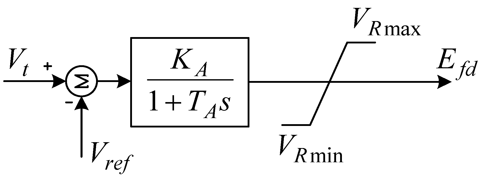
The excitation system (e.g., AVR) model is required for power system oscillatory stability analysis. An excitation system is used to regulate the generator output variables, such as voltage, power factor, and also can be used to integrate power system stabilizer (PSS). The variables are set by setting the field flux on the generator. In this research, a fast exciter system is considered. The mathematical representation of the fast exciter can be described by Equation (2).

$$E_{fd}=\frac{K_A\left(V_t-V_{ref}\right)}{1-T_{A}s}$$

(2)

In Equation (2), K_A and T_A are the gain constant and time delay constant, respectively. Furthermore, the output of the exciter is limited by the saturation block, as shown in Figure 1 [20]. The parameters of the fast excitation system are taken from [19,20], and the references therein.

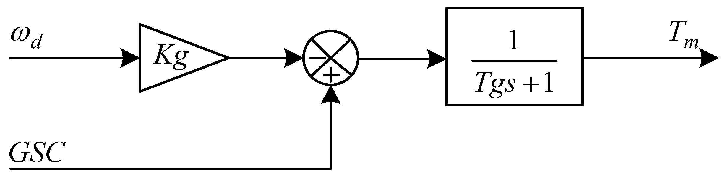
The mechanical torque of the generator depends on the speed droop constant, the time constant of the governor, and the energy source. If there is a change in the generator rotation, the governor will provide feedback to achieve a new speed (new condition). In this research, the governor has been modeled as a first-order differential equation with a gain constant, as shown in Figure 2. The first-order governor model is sufficient enough for the oscillatory stability studies due to the slow time-scale operation of the governor system [19,20]. The initial governor parameters are taken from the [19] and the references therein.

In this model, the GSC value is zero and the effect of the combination of turbine system and speed governor produces mechanical power which can be described in Equation (3). In Equation (3), K_g and T_g are gain constant and time constant of the governor [20].

$$P_m=-\left(\frac{K_g}{1+T_{g}s}\right){\omega }_d$$

(3)

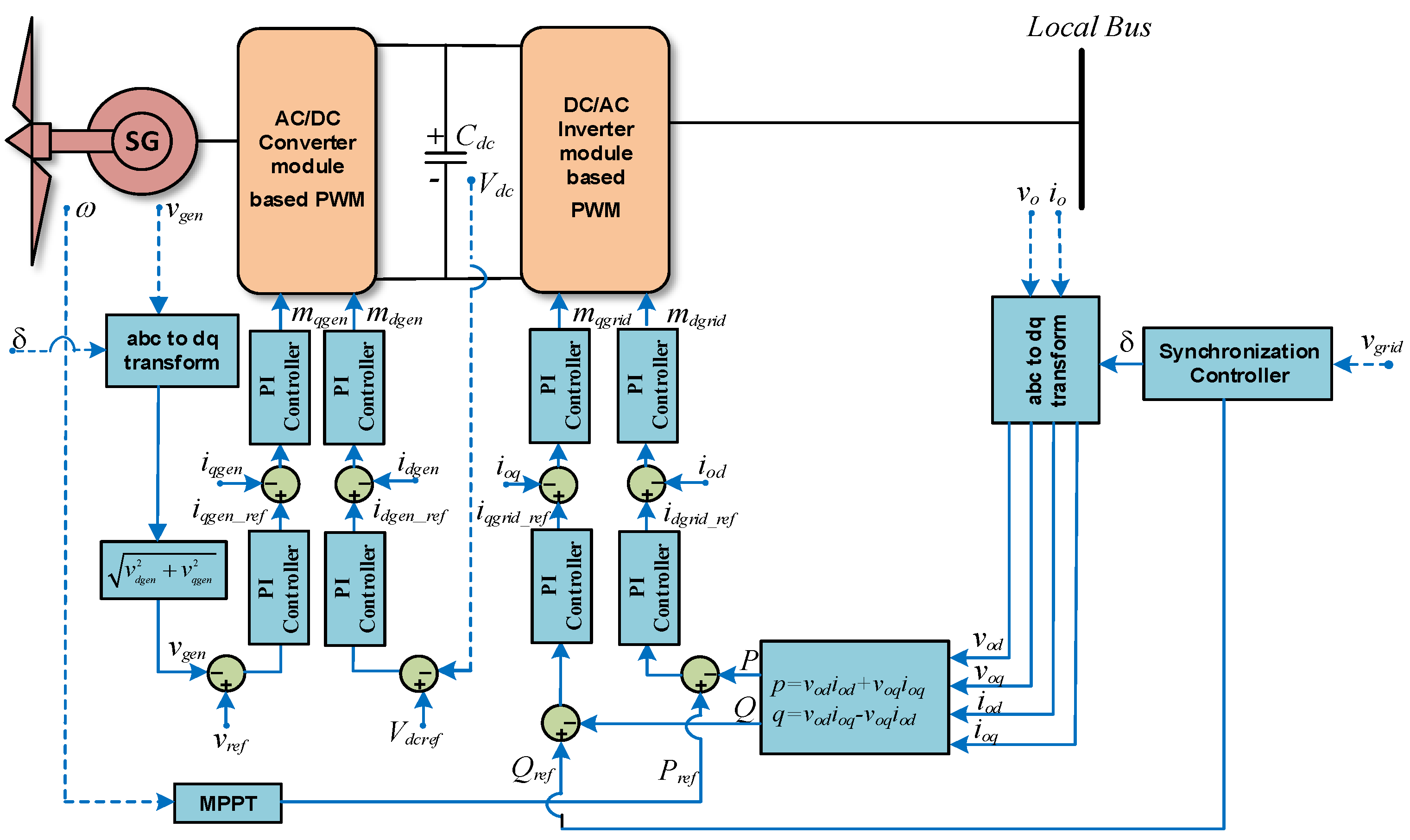
2.2. Dynamic Model of WECS

The permanent magnet synchronous generator (PMSG) based wind energy conversion systems (WECS) are considered in this work. The schematic diagram, which includes the PMSG, wind turbine, converter, associated controllers given in Figure 3, is used for the simulation. The power output as a function of wind velocity can be expressed as Equation (4).

$$P_w=c_p\frac{1}{2}\rho A{v}_w^3$$

(4)

In Equation (4), $P_w$ represents the power available from the wind, $c_{p }$ is the power coefficient, A presents the rotor swept area of the wind turbine, while, $\rho$ and $v$ represent the air density, and upstream wind speed in the rotor, respectively. The aerodynamic mechanical torque $({\tau }_w)$ associated with the wind turbine can be obtained as Equation (5) [21].

$${\tau }_w=\frac{P_w}{{\omega }_w}$$

(5)

In Equation (5), ${\omega }_w$ presents the rotor speed. For this work, the WECS system without a gearbox has been considered. Therefore, no gearbox model has been developed. Hence, the values of aerodynamic and mechanical torque transmitted to the generator are considered to be the same. Furthermore, the power coefficient of the wind turbine can be expressed by the blade pitch angle and the tip-speed ratio. The power coefficient can be expressed as in Equation (6).

$$c_p\left(\mu ,\vartheta \right)=c_1\left(c_2\frac{1}{\beta }-c_3\vartheta -c_4{\vartheta }^x-c_5\right)e^{-c_6\frac{1}{\beta }}$$

(6)

In Equation (6), $c_1-c_6$ are the coefficient, x represents the function related to the wind turbine rotor, and $\beta$ is the constant term. The values of $c_1-c_6$ and x are obtained from Equation (7) [21].

$$\frac{1}{\beta }=\frac{1}{\mu +0.08\vartheta }-\frac{0.035}{1+{\vartheta }^3}$$

(7)

In Equation (7), $\vartheta$ represents the pitch angle, $\mu$ is the tip ratio. The tip ratio $\left(\mu \right)$ can be estimated as Equation (8) [21].

$$\mu =\frac{{\omega }_{w}R}{v_w}$$

(8)

The power train model of WECS is required for oscillatory stability studies. The power train model consists of the rotor shaft, generator, blade pitching, and hub with a blade. The power train model used in this paper can be expressed as Equation (9).

$$\frac{d{\omega }_g}{dt}=\frac{{\tau }_e-{\tau }_{w\_g}}{J_{eq}}-\frac{B_m}{J_{eq}}{\omega }_g$$

(9)

In Equation (9), ${\omega }_g$ is the mechanical speed of the generator, $B_m$ denotes the damping coefficient, aerodynamic torque is represented by ${\tau }_{w\_g}$, equivalent inertia is given by $J_{eq}$, and ${\tau }_e$ is the electromechanical torque. Furthermore, the parameter of the generator side is described by sub-index, g. The comprehensive mathematical model of PMSG can be expressed by Equations (10)–(13) [21].

$$\frac{d{\omega }_g}{dt}=\frac{{\tau }_e-{\tau }_{w\_g}}{J_{eq}}-\frac{B_m}{J_{eq}}{\omega }_g$$

(10)

$$\frac{d{i}_d}{dt}=\frac{1}{L_{ds}+L_{is}}\left(-R_s{i}_d+{\omega }_e\left(L_{qs}+L_{is}\right)i_q+u_d\right)$$

(11)

$$\frac{d{i}_q}{dt}=\frac{1}{L_{qs}+L_{is}}\left(-R_s{i}_q+{\omega }_e\left[\left(L_{ds}+L_{is}\right)i_q+{\psi }_f\right]+u_d\right)$$

(12)

$${\omega }_e=p{\omega }_g$$

(13)

In Equations (10)–(13), poles are given by p, ω_e is the electrical speed, stator resistance is denoted by R_s, L_d, and L_q are the generator inductances, ψ_f is the magnetic flux, and L_id are L_iq the leakage inductances. Moreover, the electromechanical torque as given in Equation (14) is also employed in the PMSG model [22].

$${\tau }_e=1.5p\left(\left(L_{ds}+L_{is}\right)i_d{i}_q+i_q{\psi }_f\right)$$

(14)

The generator side AC/DC converter incorporates the outer and inner controllers. The outer control loop measured the terminal voltage, DC link voltage and compared those measured signals with their reference values. The signal errors are then synthesized using the conventional PI controller to derive reference values of d-axis and q-axis currents. By considering ${\beta }_{dgen}$ and ${\beta }_{qgen}$ as auxiliary state variables of the outer control loop of the generator side converter, state equations of the controller can be stated as in Equation (15) [23].

$$\frac{d{\beta }_{dgen}}{dt}=v_{dcref}-v_{dc},\frac{d{\beta }_{qgen}}{dt}=v_{gen\_ref}-v_{gen}$$

(15)

The d-axis and q-axis reference currents in the generator side can be expressed as Equations (16) and (17).

$$i_{dgen\_ref}=K_{i21}{\beta }_{dgen}+K_{p21}{v}_{dcref}-K_{p21}{v}_{dc}$$

(16)

$$i_{qgen\_ref}=K_{i11}{\beta }_{qgen}+K_{p11}{v}_{gen\_ref}-K_{p11}{v}_{gen}$$

(17)

Output variables from the outer control loop are then fed into the inner current control loop as reference values and compared with the actual values of generator currents $\left(i_{dgen},i_{qgen}\right)$. Auxiliary state variables of ${\gamma }_{dgen}$ and ${\gamma }_{qgen}$ are used to express the state equations of the inner current controllers and expressed as in Equation (18).

$$\frac{d{\gamma }_{dgen}}{dt}=i_{dgen\_ref}-i_{dgen},\frac{d{\gamma }_{qgen}}{dt}=i_{qgen\_ref}-i_{qgen}$$

(18)

A similar method is implemented to the current control loop to determine the modulation indices $\left(m_{dgen}^{*},m_{qgen}^{*}\right)$ for the generator-side converter. These modulation indices are afterward employed as control variables for the PWM scheme of the converter. Furthermore, the algebraic equations of modulation indices reference signal can be obtained as in Equations (19) and (20) [23]:

$$m_{dgen}^{*}=K_{i41}{\gamma }_{dgen}+K_{p41}{i}_{dgen\_ref}-K_{p41}{i}_{dgen}$$

(19)

$$m_{qgen}^{*}=K_{i31}{\gamma }_{qgen}+K_{p31}{i}_{qgen\_ref}-K_{p31}{i}_{qgen}$$

(20)

Similar to the generator-side control, the grid-side inverter control of WECS consists of outer and inner control loops. The active and reactive power reference values are compared to the measured active and reactive output power in the outer loop. State equations of grid side outer control loop can be derived by considering ${\beta }_{dgrid}$ and ${\beta }_{qgrid}$ as auxiliary state variables as in Equation (21).

$$\frac{d{\beta }_{dgrid}}{dt}=P_{ref}-P,\frac{d{\beta }_{qgrid}}{dt}=Q_{ref}-Q$$

(21)

The obtained error from the outer control loop is then regulated by PI controllers, yield the reference values for the inner current control loop as follows:

$$i_{dgrid\_ref}=K_{i22}{\beta }_{dgrid}+K_{p22}{P}_{ref}-K_{p22}P$$

(22)

$$i_{qgrid\_ref}=K_{i12}{\beta }_{qgrid}+K_{p12}{Q}_{ref}-K_{p12}Q$$

(23)

Moreover, the inner current control loop generated modulation indices $\left(m_{dgrid}^{*},m_{qgrid}^{*}\right)$ to provide the switching signal for the grid side inverter. Auxiliary state variables of ${\gamma }_{dgrid}$ and ${\gamma }_{qgrid}$ are required to provide state equations of the inner current control loops as given in Equation (24).

$$\frac{d{\gamma }_{dgrid}}{dt}=i_{dgrid\_ref}-i_{od},\frac{d{\gamma }_{qgrid}}{dt}=i_{qgrid\_ref}-i_{oq}$$

(24)

The algebraic equations of the reference signal for modulation indices of the grid-side inverter are given by Equations (25) and (26) [23].

$$m_{qgrid}^{*}=K_{i32}{\gamma }_{qgrid}+K_{p32}{i}_{qgrid\_ref}-K_{p32}{i}_{oq}$$

(25)

$$m_{dgrid}^{*}=K_{i42}{\gamma }_{dgrid}+K_{p42}{i}_{dgrid\_ref}-K_{p42}{i}_{od}$$

(26)

2.3. Dynamic Model of PV Generation

The transmission level PV generator model has been used in this paper. The generic model of the PV, developed by NERC, WECC, and IEEE Task Force, has been used in this study. Based on the NERC’s special report, the PV model can be consisting of the grid-side converter and control model of the type-4 wind turbine. Figure 4 shows the dynamic model of a transmission level PV system [24]. The figure shows that the power order has been used to represent the generation of PV array power.

The first-order transfer function with unity gain has been considered to represent the converter dynamics. This facilitates the current injection into the network with respect to the electrical controller’s active and reactive power command. The active power order to the system depends on the model’s power order (PPV), while the reactive power generation depends on the comparative signal generation from the reactive power control loop (e.g., q-axis loop). Three different reactive controls can be implemented in the PV system (e.g., voltage control, power factor, reactive power control) and can be interchangeable based on the flag settings in the controller [24].

The controller is comprised of PI reactive power control and converter current limits. The MPPT of PV embraces the logic algorithm to track the maximum power of the PV array. Hence, the MPPT can be neglected due to the no dynamics. The detailed presentation of the PV plant for the electromechanical time-frame analysis including the dynamic parameters can be found in [24].

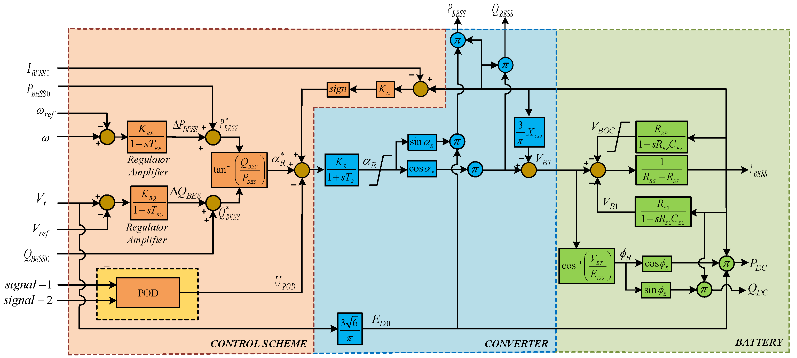
2.4. Dynamic Model of Virtual Synchronous Machine

The battery energy storage system (BESS) including virtual inertia controller is used in this paper to represent the VISMA. The BESS model consists of a second-order model with battery cells. This also includes a first-order model of converter dynamics, and a second-order model of active and reactive power control.

The active and reactive power control signal of a BESS can be obtained as Equations (27) and (28) [25].

$$\Delta P_{BESS}=\frac{k_{BP}}{1+s{T}_{BP}}\Delta \omega$$

(27)

$$\Delta Q_{BESS}=\frac{k_{BQ}}{1+s{T}_{BQ}}\Delta V_t$$

(28)

In Equations (27) and (28), K_BP represents the control loop gain and T_BP is the time constant of the active power loop. The K_BQ is the reactive power loop gain and T_BQ is the time constant of the reactive power controller. The converter dynamic can be obtained as Equations (29) and (30) [25].

$${\alpha }_R=\frac{k_R}{1+s{T}_R}\left({\alpha }_R^{*}+k_M\Delta I_{BESS}\right)$$

(29)

$${\alpha }_R^{*}={\tan }^{-1}\left(\frac{Q_{BESS}^{*}}{P_{BESS}^{*}}\right)$$

(30)

In Equations (29) and (30), K_R denotes the gain of the converter and T_R is the time delay associated with the firing angle, while, K_M and I_BESS are used to stabilize the BESS during the constant current operation so that the BESS could able to release more power from the battery banks. Moreover, $P_{BESS}^{\ast }$ and $Q_{BESS}^{\ast }$ are active and reactive power output of the converter controller. Furthermore, the battery cell dynamics are also required for this study. The dynamics model of the battery cell can be obtained as Equations (31)–(33) [25].

$$V_{BOC}=\frac{R_{BP}}{1+s{R}_{BP}{C}_{BP}}{I}_{BESS}$$

(31)

$$V_{B1}=\frac{R_{B1}}{1+s{R}_{B1}{C}_{B1}}{I}_{BESS}$$

(32)

$$I_{BESS}=\frac{1}{R_{BS}+R_{BT}}\left(V_{BT}-V_{BOC}-V_{B1}\right)$$

(33)

In Equations (31)–(33), R_BP and C_BP are the self-discharging resistance and capacitance of the battery, while R_B1 and C_B1 represent the energy and voltage in charging and discharging. Moreover, V_BOC and V_B1 represent the open-circuit voltage and overvoltage of the battery, respectively. Furthermore, V_BT, R_BS, and R_BT are the terminal voltage, the series resistance of the battery, and the equivalent resistance (e.g., parallel/series connection) of batteries. Figure 5 shows the block diagram of the BESS dynamic model used for the simulation. This is a fifth-order model of battery with converter and the controller. It should be worth noting that the given fifth-order model of battery also consists of POD to compare the proposed VISMA with respect to the auxiliary damping control in the BESS for oscillation damping. To make the BESS operate as VISMA, an additional control scheme has been added. 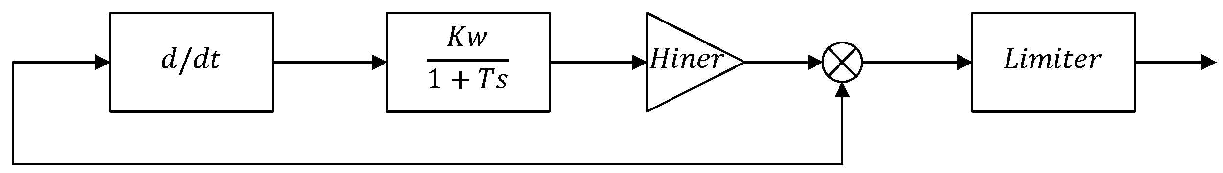Figure 6 shows the dynamic model of the virtual inertia controller [26]. The input of this controller is a frequency deviation, while the output of this controller is a reference signal of the converter.

3. Method

3.1. Extreme Learning Machine

Extreme learning machine (ELM) has become popular in recent years in addressing various engineering and other science problems. It was introduced by G. B. Huang in 2006. The ELM structure is constructed by a single hidden layer feed-forward network (SLFN). The ELM method is developed to overcome the weakness in the conventional SLFN, especially in terms of the learning process. The parameters of ELM in its hidden layer are selected randomly and do not have to be tuned. Furthermore, it can produce good generalizations. Thus, it makes the correlation between output and input data is extraordinary fast compared to the other traditional learning algorithms such as SLFN. In addition, the hidden nodes could be set up before the training samples are gained. There are two reasons behind the slow learning process of SLFN [27]. These are:

• The application of a gradient-based learning algorithm to be conducted for the training process.
• Parameters on the network are determined via iteration using this learning method.

The manual learning process is used in the gradient-based learning algorithm. The parameters in the conventional gradient-based method are the input weight and hidden bias, which are also interconnected from one layer to another. Therefore, it requires a slow learning speed process, and it is often trapped in the local minima.

The formulation of the output function of ELM for generalized SLFN is defined as follows [27]:

$$y_L\left(\mathrm{x}\right)={{\displaystyle \sum }}_{i=1}^L{\phi }_i{\psi }_i\left(\mathrm{x}\right)=\mathsf{\psi }\left(\mathrm{x}\right)\mathsf{\phi }$$

(34)

where $\mathsf{\phi }=\left[{\phi }_1, \dots , {\phi }_L\right]$^T is the vector of output weight between the hidden layer of L nodes and the output node. The $\mathsf{\psi }\left(\mathrm{x}\right)=\left[{\psi }_i\left(\mathrm{x}\right), \dots , {\psi }_L\left(\mathrm{x}\right)\right]$ is the output vector of the hidden layer with respect to x. The input data of ELM in d-dimension is mapped by $\mathsf{\psi }$(x) to L-dimensional hidden-layer feature space H.

In terms of the learning process, the ELM algorithm is different from the traditional learning algorithm where the goal of the ELM is to reach not only the smallest error value but also the smallest norm of output weights at the same time as described in (35).

$$\mathrm{minimize}:\parallel \mathrm{H}\mathsf{\phi }-\mathrm{T}{\parallel }^2,\parallel \phi \parallel$$

(35)

where H is the hidden-layer output matrix.

$$\mathrm{H}=\left[\begin{array}{c}{\psi }_{}\left({\mathrm{x}}_1\right)\\ ⋮\\ {\psi }_{}\left({\mathrm{x}}_N\right)\end{array}\right]=\left[\begin{array}{ccc}{\psi }_1\left({\mathrm{x}}_1\right)& \dots & {\psi }_L\left({\mathrm{x}}_1\right)\\ ⋮& ⋮& ⋮\\ {\psi }_1\left({\mathrm{x}}_N\right)& \dots & {\psi }_L\left({\mathrm{x}}_N\right)\end{array}\right]$$

Using Karush-Kuhn Tucker (KKT) optimality conditions, the least-squares problem of Equation (35) can be solved by Equation (36) [28].

$$\phi ={\mathrm{H}}^{\mathrm{T}}{\left(\frac{\mathrm{I}}{{\lambda }_r}+{\mathrm{HH}}^{\mathrm{T}}\right)}^{-1 }\mathrm{T}$$

(36)

where I, T, and ${\lambda }_r$ are identity matrix, target matrix, and regularization factor, respectively. The target matrix can defined as T = [t₁, …, t_N]^T.

By substituting (36) into (34), the output of ELM can be obtained as defined in Equation (37) [28]:

$$y\left(\mathrm{x}\right)=\mathsf{\psi }\left(\mathrm{x}\right){\mathrm{H}}^{\mathrm{T}}{\left(\frac{\mathrm{I}}{{\lambda }_r}+{\mathrm{HH}}^{\mathrm{T}}\right)}^{-1 }\mathrm{T}$$

(37)

3.2. Fruit Fly Optimization

The Fruit Fly Optimization (FFO) was introduced by Pan in 2011 [29]. In terms of smell and vision, fruit flies are superior compared to other similar species. Fruit flies can detect the food from 40 km away [30]. Fruit flies move toward the food according to the smell. Furthermore, they could also reach their food by using their vision capability [31].

FFO has two important steps namely the smell step and vision step. In the smell phase, the fruit flies move toward the food by using their smelling ability. Once they reached near to the food, the vision phase was established [32]. This second step is used to identify their nearest food. The fruit flies will repeat this process until they find the food. The FFO step can be described as follows [33]:

• Initialization of parameters (number of particles, number of iterations).
• Initialization of the initial position of particles.
• Update the location by using smell sensing. The mathematical representation of smell sensing can be described in Equations (38) and (39).

  $$X_i=X_{axis}+RandomValue$$

  (38)

  $$Y_i=Y_{axis}+RandomValue$$

  (39)
• Calculate the distance of the fly from the origin as well as smell concentration judge value (S). The mathematical representation of these procedures can be described using Equations (40) and (41).

  $$Dis{t}_i=\sqrt{X_i^2+Y_i^2}$$

  (40)

  $$S_i=\raisebox{1ex}{$1$}\!\left/ \!\raisebox{-1ex}{$Dis{t}_i$}\right.$$

  (41)
• Calculate the smell concentration value using Equation (42).

  $$Smel{l}_i=Function \left(S_i\right)$$

  (42)
• Detect the best fly using Equation (43).

  $$\left[bestSmell bestIndex=\max \left(Smell\right)\right]$$

  (43)
• Save the best concentrate value and the best location of fruit flies using Equations (44)–(46).

  $$Smellbest=bestSmell$$

  (44)

  $$X_{axis}=X\left(bestIndex\right)$$

  (45)

  $$Y_{axis}=Y\left(bestIndex\right)$$

  (46)
• Repeat step 3 to step 6 until the algorithm meets the specified criterion.

3.3. Tuning VISMA Using FFO

This section describes the procedure of optimizing VISMA parameters (K_w and H) using FFO. The objective function of FFO can be mathematically described using a comprehensive damping index (CDI) as given in Equation (47) [34].

$$CDI={\displaystyle \sum _{i=1}^n(1-{\zeta }_i)}$$

(47)

The procedure of tuning VISMA parameters based on FFO includes the following steps:

Step 1.

Linearize the Java-Indonesian grid with all generations and BESS around the chosen operating point.

Step 2.

Start the FFO by initializing the number of fruit flies, number of iteration, number of optimized parameters.

Step 3.

Generate random position of fruit flies as the initial position.

Step 4.

Update the location by using smell sensing.

Step 5.

Calculate the distance of the fly from the origin and estimate the smell concentration.

Step 6.

Obtain the smell concentrate value.

Step 7.

Determine the best fly based on the objective function.

Step 8.

Save the best concentration value and the best location of fruit flies.

Step 9.

Repeat step 8 until the algorithm meets the criterion (i.e., minimum iteration or objective function).

Step 10.

Print the results (K_w and H value).

3.4. Implementation of ELM and FFO

This section illustrates the process of implementing the proposed method (adaptive VISMA based on Hybrid ELM and FFO). The FFO is used here for the initial parameter tuning. The resulted parameters are then used to obtain the VISMA parameters through the ELM training process. The purpose of this process is to make the VISMA adaptive against the uncertainty of the system operating conditions. The input parameters for training are active power (P) and reactive power (Q). While the output (predicted) parameters for VISMA are K_w and H, respectively.

The procedure of adaptive VISMA includes the following steps:

Step 1.

Java-Indonesian system linearized model used in the FFO should be considered.

Step 2.

Initiate to optimize the VISMA parameters.

Step 3.

Facilitate the training data from the FFO process.

Step 4.

Conduct the training process using Equation (37).

Step 5.

Compute the accurateness of the predicted parameter using mean absolute error as Equation (48)

$$MSE={\displaystyle \sum }_{i=1}^N\frac{{\left({\tilde{y}}_i-y_i\right)}^2}{N}$$

(48)

where ${\tilde{y}}_i$ is the predicted data obtained by the proposed learning algorithm, while $y_i$ is actual data, and N is the number of data utilized in the training phase.

Step 6.

If the MSE value is minimum (meet the threshold settings), print out the results. Otherwise, go to step 4 until the minimum MSE is obtained.

4. Results and Discussions

The Java-Indonesian electric grid (i.e., 500 kV) has been used in this paper to demonstrate the efficacy of the proposed oscillation damping method. The parameters of the synchronous generators are taken from the realistic model of the Java-Indonesian grid (see Appendix A for system data). The peak load of the realistic system has been used for the simulation. Renewable power generations are considered into the Java grid to simulate the future Indonesian system—2030 scenario (60% from the conventional generators and 40% from renewable-based generations). A large-scale PV plant of 300 MW size is considered to replace a synchronous generator in area 1 (at bus 4). Moreover, an aggregated wind farm is also integrated into area 1. Furthermore, a large-scale BESS of 100 MW size is added to bus 9 in area 2, as shown in Figure 7. The PV and wind power generations are assumed to be operated at the maximum operating point.

Table 1. Damping value of Java Indonesian power grid.

Mode	Damping (%)
Inter-area	2.07
Local 1	9.07
Local 2	2.11
Local 3	6.26
Local 4	6.25
Local 5	26.84
Local 6	18.09

gives the damping performance of a 500 kV Java-Indonesian power network with PV, wind, and BESS. It is also noticeable that there are two weak modes impending from inter-area mode and local mode 2. Thus, this paper’s investigation focuses on enhancing the damping performance of these two weak modes in the system.

4.1. Training Phase

This section describes the training phase of the proposed method. The data used in this paper for the training process are given in

Table 2. Operating conditions and VISMA parameters.

P (MW)	Q (MVar)	Kw (pu)	H (s)
10,640.45	6681.436	262.2738	6.7365
10,714.21	7152.194	264.2863	6.5289
10,665.3	6681.436	261.783	6.8663
10,693.97	7160.09	261.8199	6.459
10,727.01	6731.925	262.8634	6.2692
10,715.57	6819.328	263.1746	6.1249
10,922.02	6974.017	263.8767	6.1847
10,860.37	7160.357	264.2711	6.1531
10,892.68	7111.536	262.5212	6.293
10,900.39	7161.816	262.5483	6.2456
11,003.69	6980.608	263.7096	6.271
10,639.27	7127.4	262.1302	6.1994
14,022.4	8208.116	263.8553	6.2499
12,680.33	7526.108	263.9225	6.3066
1564.689	6352.021	263.14	6.1843
10,517.13	5860.536	264.1308	6.1905
10,492.31	5605.51	264.3294	6.3298
10,488.15	5564.231	261.8926	6.1758

. The active power and reactive power is given in Table 2 are utilized as the input of ELM. Furthermore, the K_w and H (virtual inertia parameters) are the output of ELM. The values of active and reactive power are obtained from various operating conditions. While the virtual inertial parameters are the optimized parameters.

Figure 8 and Figure 9 illustrate the comparison between actual K_w and H parameters with K_w and H based on the ELM. It is noticeable that ELM can predict the value of K_w and H optimally as indicated by the pattern given in the Figures Moreover,

Table 3. Detailed features of the results are given in Figure 8.

Kw Actual	Kw ELM	Error
262.2738	262.2682	0.0056
264.2863	264.2807	0.0056
261.7830	261.7774	0.0056
261.8199	261.8143	0.0056
262.8634	262.8577	0.0057
263.1746	263.1690	0.0056
263.8767	263.8709	0.0058
264.2711	264.2654	0.0057
262.5212	262.5154	0.0058
262.5483	262.5425	0.0058
263.7096	263.7037	0.0059
262.1302	262.1247	0.0055
263.8553	263.8465	0.0088
263.9225	263.9149	0.0076
263.1400	263.1436	0.0036
264.1308	264.1253	0.0055
264.3294	264.3239	0.0055
261.8926	261.8871	0.0055

and

Table 4. Detailed features of the results are given in Figure 9.

H Inertia Actual	H Inertia ELM	Error
6.7365	6.7314	0.0051
6.5289	6.5238	0.0051
6.8663	6.8612	0.0051
6.459	6.4539	0.0051
6.2692	6.2641	0.0051
6.1249	6.1198	0.0051
6.1847	6.1796	0.0051
6.1531	6.1480	0.0051
6.293	6.2879	0.0051
6.2456	6.2405	0.0051
6.271	6.2659	0.0051
6.1994	6.1943	0.0051
6.2499	6.2452	0.0047
6.3066	6.3017	0.0049
6.1843	6.1783	0.0060
6.1905	6.1854	0.0051
6.3298	6.3247	0.0051
6.1758	6.1707	0.0051

show the detailed features of Figure 8 and Figure 9. It is found that ELM produces a minimum error for the actual parameter and predicted parameter. Moreover, it is found that the maximum error for K_w parameter is 0.0088 and the minimum error is 0.0036. In addition, it is also noticeable that the mean square error (MSE) value for the K_w parameter is 0.005817. Furthermore, the maximum and minimum errors for the H parameter are 0.0060 and 0.0047, respectively. While the MSE value for H is 0.005117.

4.2. Testing Phase

The efficacy of the proposed method is tested, compared, and discussed in this section. The aggregated active power demand of 14,022.4 MW and 8208.16 MVar reactive power demand are considered for the testing of the proposed method.

Table 5. Damping performance comparison of different scenarios.

Index	System with BESS (%)	System with VISMA (%)	System with POD at BESS (%)
Inter-area	2.24	19.74	18.63
Local 2	2.11	7.42	7.36

shows the damping comparison of the system with BESS (no POD), the system with VISMA, and the system with POD at BESS (optimized using Bat Algorithm). In this paper, only inter-area and local area 2 are used to test the efficacy of the controller as both are identified as weak modes. It is found that a system with VISMA can enhance the damping performance of weak modes significantly. It is noticeable that the inter-area mode damping enhanced from 2.24% to 19.74%, while the local mode 2 dampings increased from 2.11% to 7.42%. The results given in Table 5 show that the system experienced better damping performance for the proposed control compared to the system with BESS (no POD) and the system with POD at BESS.

To validate the results given in Table 5, non-linear time-domain simulations are carried out. The time-domain simulations are carried out by applying a small perturbation of 0.01 pu load change. Figure 10 and Figure 11 show the rotor speed responses of G3 and G4. It is found that the system with only BESS exhibits higher oscillation compared to the system with VISMA and POD at BESS. It is also observed that the oscillatory condition of the system with POD at BESS method is almost similar to the system with VISMA. Hence, this non-linear time-domain simulation validated the damping performance results given in Table 5.

Table 6. Detailed features of G3 response.

Index	System with BESS	System with VISMA	System with POD at BESS
Overshoot	−0.0000047	−0.000002742	−0.000002952
Settling time	>30	11.50	11.79

and

Table 7. Detailed features of G4 response.

Index	System with BESS	System with VISMA	System with POD at BESS
Overshoot	−0.000008852	−0.0000006257	−0.0000006958
Settling time	>30	13.00	13.15

show the detailed features of rotor speed responses of G3 and G4. It is found that systems with only BESS experience longer oscillatory conditions compared to the other scenarios. Moreover, it is noticeable that systems with actual VISMA have smaller overshoot compared to the POD at BESS. Furthermore,

Table 8. Damping value of critical EM modes under different operating conditions.

P (MW)	Q (MVar)	Inter-Area (%)	Local Mode 2 (%)
10,640.45	7143.108	19.73	7.40
10,665.296	6681.436	17.76	8.41
10,714.209	7152.194	20.00	7.40
10,693.97	7160.09	19.68	7.45
10,727.01	6731.925	17.59	10.4
10,715.57	6819.328	17.78	10.3
10,922.02	6974.017	19.48	7.42
10,860.37	7160.357	19.73	9.35
10,892.68	7111.536	19.72	9.32

shows the damping performance of the system under different operating conditions. It is found that under different operating conditions, the damping ratios investigated modes are maintained above the damping standard.

Figure 12 shows the damping ratios for different scenarios (i.e., Scenario 1: System without BESS; Scenario 2: System with BESS; Scenario 3: System with VISMA-FFO; Scenario 4: System with VISMA-proposed). The results show that the proposed method could provide better damping to the critical mode. It is worth noting that the performance of VISMA by FFO is lower compared to the proposed method.

Figure 13 and Figure 14 show the non-linear simulation results under three-phase fault at area 2 for the given scenarios in Figure 12. The results in Figure 13 and Figure 14 show that the proposed method could settle the rotor oscillation due to severe fault faster. It is worth noting that the performance of VISMA by FFO is lower compared to the proposed method.

The comparison between the proposed method (VISMA based ELM) with other tuning methods (VISMA based ANN and VISMA based PSO) is given next. Damping ratio comparison and non-linear time-domain simulation show the proposed method’s performance compared with ANN and PSO methods.

Table 9. Damping performance comparison of different methods.

Index	PSO VISMA	VISMA-ANN	VISM-ELM
Inter-area	7.42	8.37	19.74
Local 2	5.64	5.66	7.42

shows the damping comparison between VISMA based ELM, VISMA based ANN, and VISMA based PSO. It is noticeable that VISMA based ELM gives a better damping performance than the other method.

Figure 15 and Figure 16 show the non-linear time-domain simulation results comparison between the proposed method, VISMA based ANN and VISMA based PSO. It is found that the system gives the best response with the proposed method. It is found that the system with the proposed method has the lowest overshoot and the fastest settling time. Hence, the system would have a better damping margin when the system is added with VISMA based on ELM.

4.3. Robustness Analysis

Two indicators are used to assess the robustness of the system with the proposed method. The structured singular value (SSV) is used as the first indicator. The SSV can be used to examine the robustness of the system against uncertainty. The paper states that the system consists of large-scale PV and wind power plants with intermittency in output. Therefore, it is essential to evaluate the robust stability against uncertainty. The generalized technique for robustness assessment using the linear fractional transformation (LFT) is depicted in Figure 17, where M indicates the complex transfer matrix. The complex transfer matrix can be described as described in Equation (49).

$$M=\left[\begin{array}{cc}{M}_{11}& M_{12}\\ M_{21}& M_{22}\end{array}\right]\in C^{\left(p_1+p_2\right)\times \left(q_1+q_2\right)}$$

(49)

In Equation (49), $\Delta \in C^{\left(q_1+p_1\right)}$ is another complex matrix. Moreover, w and z are the vectors of perturbation output and input. The upper LFT with respect to $\Delta$ can be described as in Equation (50).

$$F_u\left(M,\Delta \right):=M_{22}+M_{21}\Delta {\left(I-M_{11}\Delta \right)}^{-1}{M}_{12}$$

(50)

In Equation (50), the unperturbed system and the nominal transfer matrix knowledge due to the perturbation is labeled as M₂₂, M₁₂, M₁₁, and M₂₁, while $\Delta$ is the perturbation. Furthermore, all sources of uncertainties can be represented by the transfer matrix $\Delta$. The mathematical representation of $\Delta$ is presented in Equation (51).

$$\Delta =\left\{diag\left[{\delta }_1{I}_{r1},\dots \dots ,{\delta }_s{I}_{rs},{\Delta }_1,\dots \dots \dots {\Delta }_F\right]\right\}$$

(51)

In Equation (51), the number of full blocks, repeated scalar blocks, and identity matrix is denoted by ${\Delta }_F$, ${\delta }_s$ and $I_{rs}$, ${\delta }_s\in R,{\Delta }_s\in C^{m_s\times m_s}$. Moreover, the smallest structured uncertainty $\Delta$ is defined as SSV. Furthermore, the SSV or µ can be expressed as in Equation (52).

$$\mu {\left(M\right)}^{-1}:=\min \left\{\overline{\sigma }(\Delta ):\Delta \in ,\det \left(I-M\Delta \right)=0\right\}$$

(52)

In Equation (52), $\mu \left(M\right)$ determines the robustness of the system. According to LFT, the system can be specified as a robustly stable system if and only if $max\mu \left(M\right)<1$. The following steps can be used for the SSV analysis in the power system:

Step 1.

Non-linear system should be linearized around the selected operating points.

Step 2.

Define the uncertainty (this could be the number of operating conditions, penetration levels of renewable generations, and others).

Step 3.

Obtain the matrix A with different uncertainty by a certain interval.

Step 4.

Get the ${\delta }_s$ (that will also vary within the interval of different uncertainty. Hence the ${\delta }_s$ can be used to capture the variation of uncertainty).

Step 5.

Estimate the $\Delta$ by using Equation (51).

Step 6.

Obtain $F_u\left(M,\Delta \right)$ by using Equation (50)

Step 7.

Calculate $\mu \left(M\right)$ by using Equation (52).

The details about the SSV calculation can be found in [35] and the references therein. The second indicator is the transient kinetic energy (TKE) assessment. The TKE assessment estimates the amount of mechanical energy used by the system in the transient condition. The smaller the value, the less the mechanical energy being used. The TKE can be estimated as in Equation (53).

$$TKE={\displaystyle \sum _{i=1}^n\frac{1}{2}{J}_i\cdot \Delta {\omega }_i^2}$$

(53)

In Equation (53), the angular momentum of the rotor at synchronous speed and speed deviation of ith generator in a system with n machines are described as J_i and Δω_i.

Table 10. SSV assessment results.

Mode	SSV
With BESS	1.5324
With proposed VISMA	0.0853
VISMA (FFO)	0.487
With POD at BESS	0.695

shows the SSV values comparison between the system with BESS only, the system with the proposed controller method, and the POD at BESS. It is found that the system with BESS has SSV above 1, while the system with the proposed controller method exhibits an SSV value well below 1. Moreover, the system with POD at BESS and VISMA by FFO shows an SSV value lower than 1. However, the SSV values of the system with POD at BESS and VISMA by FFO are higher than the system with the proposed method. Hence, it can be stated that the proposed controller can make the system robust against uncertainty. Moreover,

Table 11. TKE comparison under different scenarios.

Index	System with BESS	System with VISMA	System with POD at BESS	System with VISMA (FFO)
G3	0.0000000000828	0.0000000000304	0.0000000000335	0.0000000000314
G4	0.0000000002155	0.00000000011309	0.0000000001331	0.00000000013309

shows the TKE value comparison for G3 and G4. It is noticeable that the TKE value for both G3 and G4 are smaller when the proposed controller method is added to the system.

5. Conclusions

This paper proposed an optimal method to design an adaptive VISMA based on ELM to enhance the small-signal stability of a renewable-rich realistic representative power system. From the simulation results, it is found that the ELM can estimate the optimal parameters for VISMA. In addition, by using ELM, VISMA can automatically adjust the parameters when there is a sudden change in the operating condition. Therefore, it exhibits better performance than the VISMA by FFO. It is worth noticing that the proposed method is also superior compared to other tuning methods for VISMA (e.g., VISMA based PSO and VISMA based ANN). Moreover, the VISMA design using ELM can handle the uncertainty in the power system as indicated by the value of the SSV (the SSV value is below 1). Furthermore, it is also found that by using VISMA based ELM, the kinetic energy produced by the system is smaller compared to the other method for both generators 3 and 4 (0.0000000000304 for G3 and 0.00000000011309 for G4).

References

1. Pitteloud, J.D. Global Wind Installations 2020. Available online: https://www.woodmac.com/press-releases/global-wind-power-installations-hit-record-levels-in-2020/ (accessed on 9 January 2022).
2. Alzubaidi, M.; Hasan, K.; Meegahapola, L.; Rahman, M.T. Identification of efficient sampling techniques for probabilistic voltage stability analysis of renewable-rich power system. Energies 2021, 14, 2328. [Google Scholar] [CrossRef]
3. Topić, D.; Vezmar, S.; Spajić, A.; Šljivac, D.; Jozsa, L. Positive and negative impacts of renewable energy sources. Int. J. Electr. Comput. Eng. Syst. 2014, 5, 15–23. [Google Scholar]
4. Yorino, N.; Abdillah, M.; Sasaki, Y.; Zoka, Y. Robust power system security assessment under uncertainties using bi-level optimization. IEEE Trans. Power Syst. 2017, 1, 352–362. [Google Scholar] [CrossRef]
5. Ma, J.; Qiu, Y.; Li, Y.; Zhang, W.; Song, Z.; Thorp, J.S. Research on the impact of DFIG virtual inertia control on power system small-signal stability considering the phase-locked loop. IEEE Trans. Power Syst. 2017, 32, 2094–2105. [Google Scholar] [CrossRef]
6. Wang, Z.; Shen, C.; Feng, L. Probabilistic analysis of small signal stability for power systems with high penetration of wind generation. IEEE Trans. Sustain. Energy 2016, 7, 1–12. [Google Scholar] [CrossRef]
7. Constante-Flores, G.E.; Illindala, M. Data-driven probabilistic power flow analysis for a distribution system with renewable energy sources using monte carlo simulation. In Proceedings of the 2017 IEEE/IAS 53rd Industrial and Commercial Power Systems Technical Conference (I&CPS), Niagara Falls, ON, Canada, 6–11 May 2017; pp. 1–8. [Google Scholar] [CrossRef]
8. Quintero, J.; Vittal, V.; Heydt, G.T.; Zhang, H. The impact of increased penetration of converter control-based generators on power system modes of oscillation. IEEE Trans. Power Syst. 2014, 29, 2248–2256. [Google Scholar] [CrossRef]
9. Eftekharnejad, S.; Vittal, V.; Heydt, G.T.; Keel, B.; Loehr, J. Small signal stability assessment of power systems with increased penetration of photovoltaic generation: A case study. IEEE Trans. Sustain. Energy 2013, 4, 960–967. [Google Scholar] [CrossRef]
10. Setiadi, H.; Mithulananthan, N.; Shah, R. Design of wide-area POD with resiliency using modified DEA for power systems with high penetration of renewable energy. IET Renew. Power Gener. 2018, 13, 342–351. [Google Scholar] [CrossRef]
11. Dhundhara, S.; Verma, Y.P. Capacitive energy storage with optimized controller for frequency regulation in realistic multisource deregulated power system. Energy 2018, 147, 1108–1128. [Google Scholar] [CrossRef]
12. Akram, U.; Khalid, M. A coordinated frequency regulation framework based on hybrid battery-ultracapacitor energy storage eechnologies. IEEE Access 2018, 6, 7310–7320. [Google Scholar] [CrossRef]
13. Pappachen, A.; Fathima, A.P. Load frequency control in deregulated power system integrated with SMES–TCPS combination using ANFIS controller. Int. J. Electr. Power Energy Syst. 2016, 82, 519–534. [Google Scholar] [CrossRef]
14. Kerdphol, T.; Rahman, F.S.; Mitani, Y.; Watanabe, M.; Küfeoǧlu, S.K. Robust virtual inertia control of an islanded microgrid considering high penetration of renewable energy. IEEE Access 2017, 6, 625–636. [Google Scholar] [CrossRef]
15. Sakr, W.S.; El-Sehiemy, R.A.; Azmy, A.M. Optimal allocation of TCSCs by adaptive DE algorithm. IET Gener. Transm. Distrib. 2016, 10, 3844–3854. [Google Scholar] [CrossRef]
16. Ali, E.S. Optimization of power system stabilizers using BAT search algorithm. Int. J. Electr. Power Energy Syst. 2014, 61, 683–690. [Google Scholar] [CrossRef]
17. Chitara, D.; Niazi, K.R.; Swarnkar, A.; Gupta, N. Cuckoo search optimization algorithm for designing of a multimachine power system stabilizer. IEEE Trans. Ind. Appl. 2018, 54, 3056–3065. [Google Scholar] [CrossRef]
18. Wang, N.; Zhang, J.; He, Y.; Liu, M.; Zhang, Y.; Chen, C.; Gu, Y.; Ren, Y.N. Load-frequency control of multi-area power system based on the improved weighted fruit fly optimization algorithm. Energies 2020, 13, 437. [Google Scholar] [CrossRef] [Green Version]
19. Vittal, V.; McCalley, J.D.; Anderson, P.M.; Fouad, A.A. Power System Control and Stability; John Wiley & Sons: Hoboken, NJ, USA, 2019. [Google Scholar]
20. Kundur, P. Power System Stability and Control; McGraw-Hill: NewYork, NY, USA, 1994. [Google Scholar]
21. Meegahapola, L.; Bu, S. Wind power integration into power systems; Stability and control. Energies 2020, 14, 2328. [Google Scholar]
22. Setiadi, H.; Krismanto, A.U.; Mithulananthan, N.; Hossain, M.J. Modal interaction of power systems with high penetration of renewable energy and BES systems. Int. J. Electr. Power Energy Syst. 2018, 97, 385–395. [Google Scholar] [CrossRef]
23. Krismanto, A.U.; Sulistiawati, I.B.; Limpraptono, F.Y.; Priyadi, A.; Setiadi, H.; Abdillah, M. Impact of large-scale wind power penetration on dynamic voltage stability of interconnected power system: An Indonesia case study. Int. J. Intell. Eng. Syst. 2021, 14, 251–263. [Google Scholar] [CrossRef]
24. Clark, K.; Miller, N.W.; Walling, R. Modeling of GE Solar Photovoltaic Plants for Grid Studies; General Electric International, Inc.: Schenectady, NY, USA, 2010; Volume 12345. [Google Scholar]
25. Chandra, S.; Gayme, D.F.; Chakrabortty, A. Coordinating wind farms and battery management systems for inter-area oscillation damping: A frequency-domain approach. IEEE Trans. Power Syst. 2013, 29, 1454–1462. [Google Scholar] [CrossRef]
26. Kerdphol, T.; Watanabe, M.; Hongesombut, K.; Mitani, Y. Self-adaptive virtual inertia control-based fuzzy logic to improve frequency stability of microgrid with high renewable penetration. IEEE Access 2019, 7, 76071–76083. [Google Scholar] [CrossRef]
27. Liu, B.; Chen, G.; Lin, H.-C.; Zhang, W.; Liu, J. Prediction of IGBT junction temperature using improved cuckoo search-based extreme learning machine. Microelectron. Reliab. 2021, 124, 114267. [Google Scholar] [CrossRef]
28. Pi, P.; Lima, D. Gray level co-occurrence matrix and extreme learning machine for COVID-19 diagnosis. Int. J. Cogn. Comput. Eng. 2021, 2, 93–103. [Google Scholar] [CrossRef]
29. Pan, W.-T. A new fruit fly optimization algorithm: Taking the financial distress model as an example. Knowl. Based Syst. 2012, 26, 69–74. [Google Scholar] [CrossRef]
30. Mitić, M.; Vuković, N.; Petrović, M.; Miljković, Z. Chaotic fruit fly optimization algorithm. Knowl. Based Syst. 2015, 89, 446–458. [Google Scholar] [CrossRef]
31. Li, Y.; Han, M. Improved fruit fly algorithm on structural optimization. Brain Inform. 2020, 7, 1–13. [Google Scholar] [CrossRef] [PubMed]
32. Fan, Y.; Wang, P.; Heidari, A.A.; Wang, M.; Zhao, X.; Chen, H.; Li, C. Rationalized fruit fly optimization with sine cosine algorithm: A comprehensive analysis. Expert Syst. Appl. 2020, 157, 113486. [Google Scholar] [CrossRef]
33. Darvish, A.; Ebrahimzadeh, A. Improved fruit-fly optimization algorithm and its applications in antenna arrays synthesis. IEEE Trans. Antennas Propag. 2018, 66, 1756–1766. [Google Scholar] [CrossRef]
34. Setiadi, H.; Mithulananthan, N.; Shah, R.; Raghunathan, T.; Jayabarathi, T. Enabling resilient wide-area POD at BESS in Java, Indonesia 500 kV power grid. IET Gener. Transm. Distrib. 2019, 13, 3734–3744. [Google Scholar] [CrossRef]
35. Mithulananthan, N.; Shah, R.; Lee, K.Y. Small disturbance angle stability control with high penetration of renewable generations. IEEE Trans. Power Syst. 2014, 29, 1463–1472. [Google Scholar] [CrossRef]
Figure 1. Schematic diagram of fast exciter [20].
Electronics 11 00247 g001
Figure 2. Schematic diagram of the governor.
Electronics 11 00247 g002
Figure 3. Schematic diagram of WECS based on PMSG.
Electronics 11 00247 g003
Figure 4. Dynamic model of the PV plant [24].
Electronics 11 00247 g004
Figure 5. Schematic diagram of fifth-order model BESS with POD.
Electronics 11 00247 g005
Figure 6. Schematic diagram of virtual inertia controller.
Electronics 11 00247 g006
Figure 7. Java Indonesian Power Grid with PV, wind, and BESS.
Electronics 11 00247 g007
Figure 8. Comparison of actual Kw data and ELM Kw data.
Electronics 11 00247 g008
Figure 9. Comparison of actual H data and ELM H data.
Electronics 11 00247 g009
Figure 10. Rotor speed responses of G3.
Electronics 11 00247 g010
Figure 11. Rotor speed responses of G4.
Electronics 11 00247 g011
Figure 12. Damping of different scenarios (Scenario 1: System without BESS; Scenario 2: System with BESS; Scenario 3: System with VISMA-FFO; Scenario 4: System with VISMA-proposed).
Electronics 11 00247 g012
Figure 13. Rotor speed responses of G3 under three-phase fault (Scenario 1: System without BESS; Scenario 2: System with BESS; Scenario 3: System with VISMA-FFO; Scenario 4: System with VISMA-proposed).
Electronics 11 00247 g013
Figure 14. Rotor speed responses of G4 under three-phase fault (Scenario 1: System without BESS; Scenario 2: System with BESS; Scenario 3: System with VISMA-FFO; Scenario 4: System with VISMA -proposed).
Electronics 11 00247 g014
Figure 15. Rotor speed responses of G3 under different methods.
Electronics 11 00247 g015
Figure 16. Rotor speed responses of G4 under different methods.
Electronics 11 00247 g016
Figure 17. Structure of robustness analysis using SSV [35].
Electronics 11 00247 g017