Using Stochastic Computing for Virtual Screening Acceleration

Abstract

Stochastic computing is an emerging scientific field pushed by the need for developing high-performance artificial intelligence systems in hardware to quickly solve complex data processing problems. This is the case of virtual screening, a computational task aimed at searching across huge molecular databases for new drug leads. In this work, we show a classification framework in which molecules are described by an energy-based vector. This vector is then processed by an ultra-fast artificial neural network implemented through FPGA by using stochastic computing techniques. Compared to other previously published virtual screening methods, this proposal provides similar or higher accuracy, while it improves processing speed by about two or three orders of magnitude.

1. Introduction

Due to the data explosion that has taken place in all scientific and technological areas, the use of artificial intelligence (AI) arises as an optimal and quick strategy to convert raw data into useful information. This data explosion is particularly critical in the area of organic chemistry, owing to the truly vast possibilities for constructing chemical compounds [1]. Such a vast chemical space embraces, but it is by no means limited to, the ever-increasing number of compounds from different chemical databases, which is now of the order of tens of billions and publicly available. For the specific problem of the analysis of interactions between different molecules—the aim of any drug discovery process, after all—the number of possibilities explodes and becomes unmanageable. This is critical, even if machine learning techniques are applied in the context of fast-growing screening libraries [2,3]. That is why speeding up this type of process by means of accelerator methods is highly desirable.

Drug development is a time-consuming process, where, on average, more than ten years and hundreds of millions of U.S. dollars are needed. From the early 1990s, huge libraries of compounds have been made available to facilitate compound screening. To aid in the early stages of the drug discovery process, new computing strategies were developed (virtual screening—VS) [4]. The primary goal of VS [5,6,7] is to find out, from a molecule database, a subset of molecules with a high chance to be chemically active. This subset of compounds is revised by medicinal chemists to improve their preclinical properties. When a 3D structure of the target is available and the binding site is known, this problem is more specifically called structure-based VS [8,9,10]. On the other hand, when at least a molecule with activity for the target compound is known, methods for ligand-based VS are used [11,12,13]. Certain ligand-based methods used for virtual screening benefits from a set of molecules [14,15,16] instead of a single ligand used as a search template. Such models are typically generated with machine learning algorithms trained on ligands with known activity [17,18].

1.1. Artificial Neural Networks Applied to Virtual Screening

It is well known that the use of advanced machine learning methodologies in VS, such as support vector machines or artificial neural networks (ANN), is becoming increasingly popular in ligand-based VS strategies [19]. ANN are inspired by how the brain processes information and have become trendy in many science and technological areas, due to their ability to solve many complex pattern matching problems. ANN can be applied to adjust complex relationships without considering the underlying physical links. A sufficiently large dataset of samples suffices to correlate the data, which consists of pairs of an input (a sample) and an output (its class). ANN are normally structured as a set of interconnected elementary processing units, each one implementing a non-linear operation. Because of the large configurability of ANN, a huge number of training examples are required for the adjustment of the connectivity matrices ${\mathsf{\Omega }}^k=\left\{{\omega }_{ij}^k\right\}$. This adjustment is specially easy to obtain for feedforward neural networks. Given a specific training dataset whose desired network response is correlated with the input, the optimization of $\mathsf{\Omega }$ is a non-convex problem that can be solved by using the backpropagation algorithm.

Neuromorphic hardware (NH) is a research field which has been propelled by the need of developing high-performance AI systems [20,21,22,23,24]. NH is able to provide timely responses to those applications which require processing huge amounts of data [25]. Many efforts have been made in implementing neuromorphic digital [26] and analogue [27] circuits. The great advantage of digital implementation is its ability to create massive ANN devices on a single chip and to easily test them in field programmable gate arrays (FPGAs) [28,29]. Nevertheless, the use of large numbers of multipliers, necessary to reproduce the neural weights, constrains its proper parallelization and, as a consequence, it limits the speeding up process.

A possible solution is the use of approximate multipliers that are built by using non-deterministic computing methods. In this particular context, stochastic computing (SC) arises as a potential alternative [30,31]. SC has been used to develop many different complex tasks, such as the implementation of Bayesian classifiers [32,33], image processing [34,35], or the implementation of neuromorphic circuits [36,37]. Data representation within the SC paradigm is performed in a probabilistic way with the use of Boolean quantities, which switch randomly over time. The probability of a single bit in a given state is used to encode the desired signal, thus reducing the area cost since only one wire is needed to carry the whole numerical value with this probabilistic codification. Hence, complex functions whose implementation requires a high amount of area, such as multiplications [38], are performed by using a single logic gate, with great savings in terms of area and power [39,40]. However, this area reduction has a cost in terms of precision loss. This is not critical anyway in most machine learning applications (e.g., ANN), where a relatively reduced set of output categories or classes must be discriminated based on generic similarities. Indeed, most of the current machine learning applications use a small number of bits to represent digitized signals [41] because the difference in the final result between using high-precision floating-point signals and low-precision 8/16-bit signals is negligible [42]. Hence, the integration time used to evaluate the result of stochastic operations can be considerably reduced since it is exponentially dependent on the bit precision. In addition, as a result of the low area employed in SC, different ANN cores can be implemented in parallel on a single chip, thus increasing the throughput, compared with traditional computing methods. Be that as it may, tackling the miscalculation produced by stochastic correlation signals remains a challenge for SC designers. The main obstacle is the high number of random number generators (RNG) needed, which are essential for producing the probabilistic bit streams used in SC. Indeed, some operations, such as multiplications, require the inputs to be uncorrelated (statistically independent) if we want to achieve accurate calculations. That is the reason why independent RNGs are necessary to generate each stochastic signal. This fact makes these blocks occupy up to the 90% of the whole area of the final circuit footprint [43], limiting the benefits of SC. It is therefore crucial to minimize the use of RNG in SC systems and simultaneously maintain the accuracy.

1.2. Objective of the Paper

In this work, we present an ultra-fast virtual screening method based on an ANN implemented with stochastic computing. The process scheme is shown in Figure 1, where we compare a known compound that presents a certain biological activity, with a set of query compounds with unknown activities (database). The proposed system provides, for each query compound, a likelihood value, which measures if the query compound presents the same activity as the active one. In this process, the following must be considered:

−

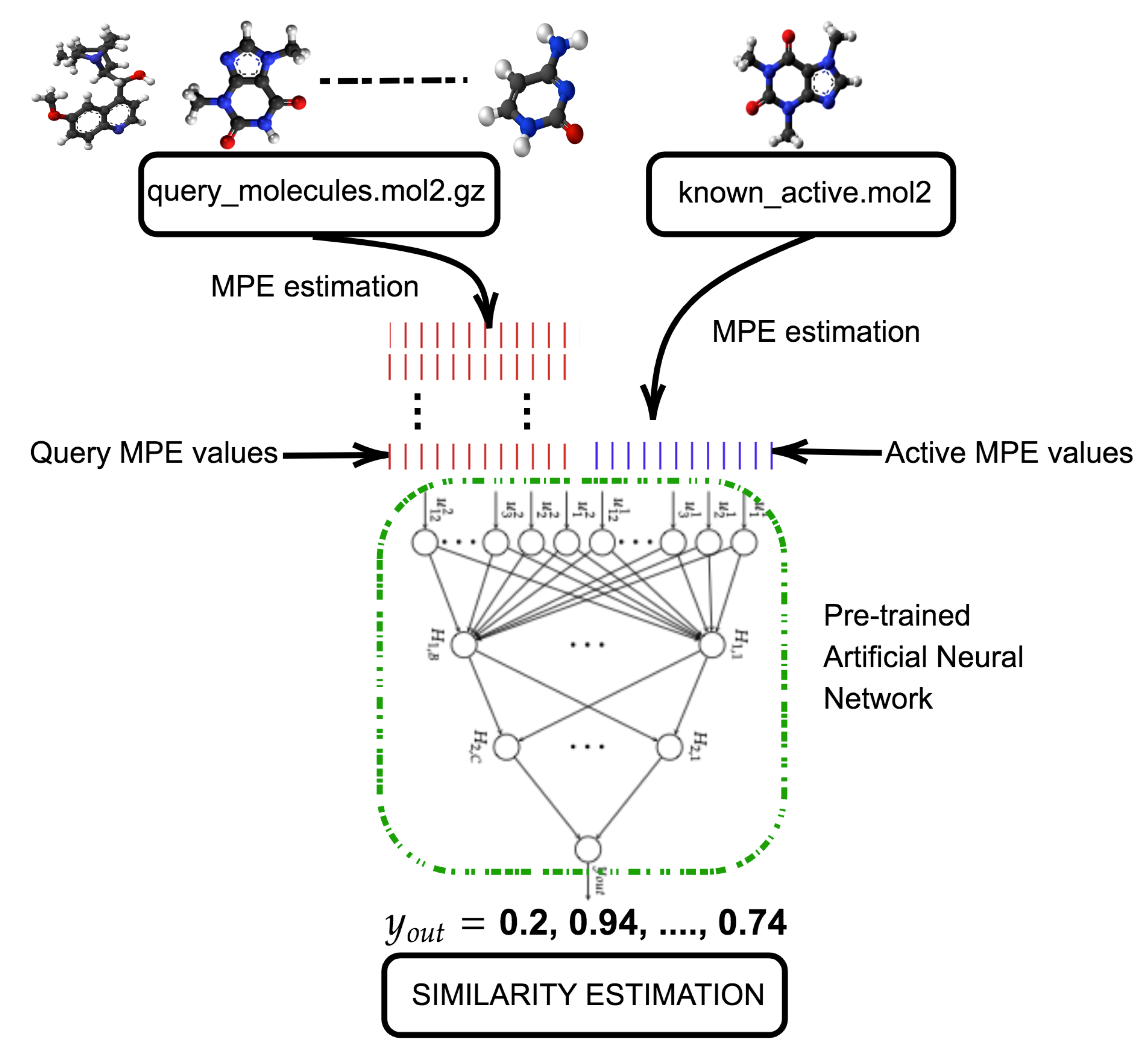
Electron distribution assigned to individual atoms must be taken into consideration along with their spacial distribution. The MOL2 file type is therefore needed for each compound since this information is included in this format.

−

A set of molecular descriptors are estimated from the MOL2 files. Molecular pairing energies (MPE) [44], dependent on both charge distribution and molecular geometry, are adopted as descriptors. These descriptors are independent of rotations and translations of the compound, and provide valuable information about its binding possibilities.

−

Once the MPE values are obtained from the query and active compounds, a preconfigured ANN estimates the similarity between queries and active compounds.

−

The database is finally ordered, according to the similarity values provided by the system and, consequently, only the top-most compounds are selected for laboratory assays.

To validate the model, we use the DUD-E dataset of chemical compounds [45]. The DUD-E docking benchmark is a widely used database to evaluate virtual screening methods. It is composed of 102 different pharmaceutical targets that include a crystal ligand, along with a set of active compounds and decoys (assumed as non-actives). The performance of the system is evaluated through the area under the curve (AUC) of the receiver operating characteristic (ROC) curve. As it will be shown, a competitive accuracy in regard to other ligand-based models present in the literature is obtained, along with good performance in terms of both processing speed and energy efficiency.

2. Methods

2.1. Molecular Pairing Energies Descriptors

Virtual screening consists of comparing each query compound of a database with active ligands against a specific target [17,18]. This comparison is normally made by using molecular descriptors that can be based on physicochemical properties. In this work, we propose a classification model which uses molecular pairing energies (MPEs) as the main descriptor [44] together with a neural network discriminator. These pairing energies are defined as

$$E_{ij}=K\frac{q_i{q}_j}{r_{ij}}$$

(1)

where $q_i$ and $q_j$ are the partial charges of each atom of the molecule, and $r_{ij}$ is the distance between them.

These partial charges are related to the electron distribution that can be assigned to individual atoms through quantum mechanical calculations. To screen thousands or millions of compounds, there are much faster and more efficient methods, such as the partial equalization of orbital electronegativity or the Merck molecular force field [46,47,48].

Among all the pairing energies present in a compound, we choose the N highest (positive) and lowest (negative) energies, thereby creating an ordered 2N-dimensional vector for the description of the molecule. If we have less than 2N pairing energies, the vector is center-padded with zeroes until it reaches the 2N dimensions. In this work, we set N to 6, so we use a total of 12 energy descriptors per compound. The most electropositive or electronegative MPE values are related to molecular scattering or the assembly properties of the compound.

In this work, the MPE model is applied to the full DUD-E database, in which the partial charges are estimated by using the MMFF94 force field [48], which is implemented within the Openbabel software. Empirically, the MPE model shows a good capability to cluster those compounds showing similar chemical properties [44], as it can be appreciated in Figure 2, where we have plotted the most positive and most negative pairing energies for five different DUD-E targets. Figure 2 suggests that those compounds with a higher cohesion energy usually have a higher scattering energy. The working hypothesis is that MPE values can be efficiently used to compare chemical activities between compounds. This way, an AI-assisted model, such as the ANN proposed, may take advantage of this representation and obtain good results.

2.2. Artificial Neural Network Implementation

ANN has emerged as a powerhouse for prediction and classification tasks. In this work, ligand-based virtual screening is seen as a classification problem to be solved via an ANN-based algorithm.

Each neuron in the network computes a transfer function of its weighted inputs so that the output of the $j^{th}$ neuron is

$$a_j=\varphi \left(\sum _i{\omega }_{ij}{x}_i\right),$$

(2)

where ${\omega }_{ij}$ is the weight assigned to the $i^{th}$ input $x_i$ and $\varphi$ is the non-linear activation function. It is supposed that all the inputs come from the previous neural layer.

Several activation functions have been used in the literature. Among them, the ReLU function ($\varphi \left(x\right)=max(x,0)$) is one of the most widely used functions due to its simplicity for both inference and training. The ReLU function has two great advantages. First, it addresses the vanishing gradient problem introduced by other activation functions during the backpropagation training phase [49]; second, it can be easily implemented in stochastic computing by using a reduced set of logic gates.

The main purpose of this work is to develop an accurate and energy-efficient methodology to implement a ligand-based virtual screening process. Starting from 24 MPE values (12 per each compound to be compared), we studied several ANN architectures with a single output (i.e., 1 and 0, meaning active and decoy, respectively) in order to estimate the target similarity. Figure 3 shows the scheme of the ANN architecture employed, in which the parameter $u_j^k$ stands for the $j^{th}$ component of the $k^{th}$ compound, $H_{l,j}$ stands for the $j^{th}$ neuron in the $l^{th}$ hidden layer, and the output $y_{out}$ is the prediction of the similarity between the compounds.

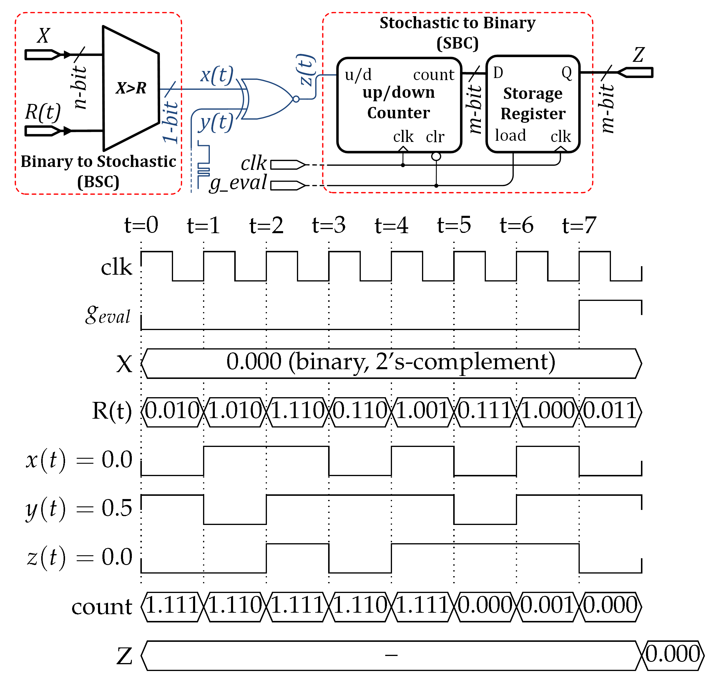
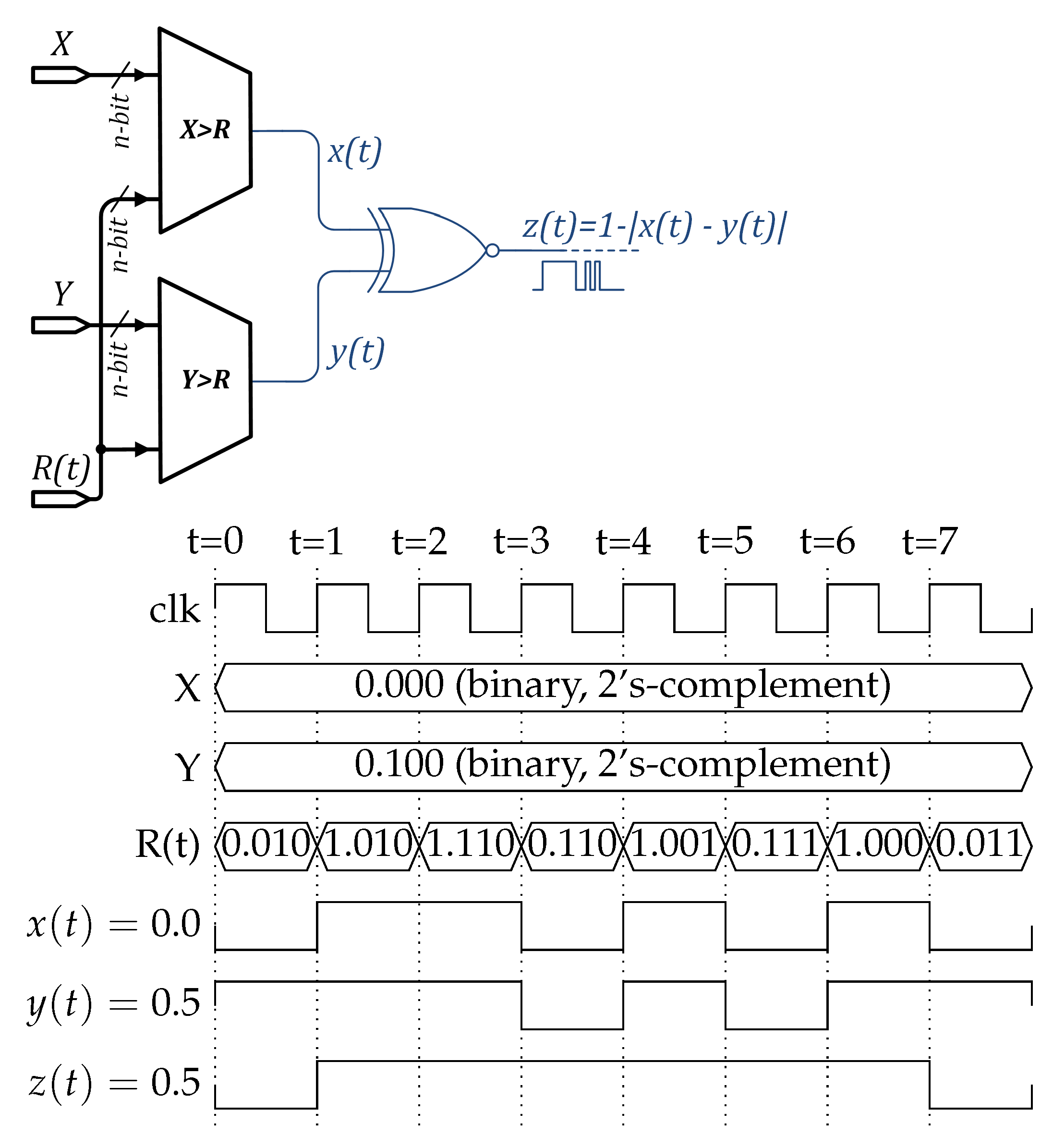
2.3. Stochastic Computing

Stochastic computing consists of representing signals by using random bit streams (BS) of length N [30,50]. There are various types of numeric codifications, being that the unipolar and bipolar are the two most important ones. In the unipolar codification, a number is directly represented by the probability of receiving a logical 1 through a wire and, as a result, the numbers that can be represented lie between 0 and 1. In the bipolar codification, a N-bit stream (BS) represents a quantity defined as $p=(N_1-N_0)/(N_0+N_1)$, being that $N_0$ and $N_1$ are the number of zeroes and ones which form the bit stream, respectively (with $N=N_0+N_1$). Thus, bipolar values are restricted between −1 and +1. In the bipolar codification, any two’s complement number X can be converted into a stochastic bit stream $x\left(t\right)$ by comparing the X value with a random number generator (RNG) $R\left(t\right)$. This way, each stochastic signal must be understood as a sequence of Booleans $x\left(t\right)=\{X>R(t\left)\right\}$, where the precision of these signals is related to the bit stream length considered (N). The RNG $R\left(t\right)$ must be uniformly distributed over the interval of all possible values of X, from $-2^{(n-1)}$ to $2^{(n-1)}-1$, being that n is the binary bit precision. To recover the original value X in the binary domain, a signed up/down counter and a register are used.

One of the main advantages of SC is the low cost in terms of hardware resources to implement complex functions. The clearest example is the stochastic multiplier: the product operation is performed by a single XNOR gate when using bipolar coding. Figure 4 illustrates a bipolar SC multiplication with the main parts of a SC system: the binary to stochastic conversion, the stochastic operation, and the recovery of the binary result. A binary signal X is converted to a stochastic $x\left(t\right)$ by using a time-varying random number $R\left(t\right)$ and a binary comparator. As a result, a single stochastic bit is obtained during each clock cycle, where SC signals are set to ‘1’ or ‘0’ with a given probability. Note that in the example of Figure 4, we multiply two SC signals $x\left(t\right)$ and $y\left(t\right)$ to generate $z\left(t\right)$). For the stochastic product operation, both input signals must be uncorrelated. It means that the covariance between signals must be zero: $Cov\left(x\left(t\right),y\left(t\right)\right)=0$. The output signal $z\left(t\right)$ is generated after applying the truth table of an XNOR gate, as shown in Figure 4. The final averaged value after the evaluation time (eight cycles in the example of Figure 4) is the product between x and y. To store the result in memory, a conversion must be carried out from the time-dependent stochastic domain to the two’s complement one. This conversion is easily performed by using a signed up/down counter and a register, which stores the final value, where at every N clock cycles (namely, the evaluation time), the enable signal $g\_eval$ is set to store the expected result.

As previously mentioned, decorrelation between SC signals is necessary for the operation to be accurate. Otherwise, the XNOR gate stops estimating the product operation. For instance, if input signals are completely correlated (i.e., when both signals are generated by the same random source), the outcome is a function associated to the absolute value of the difference between the input signals (see Figure 5). Therefore, maximum correlation between SC signals is attained when bit streams are generated using the same RNG, as shown in Figure 5. To quantify the degree of correlation, the following expression is normally used [51]:

$$C(x,y)=\frac{Cov\left(x\left(t\right),y\left(t\right)\right)}{1-\mid x-y\mid -xy},$$

(3)

where the function $Cov$ is the covariance between two time-dependent stochastic signals $x\left(t\right)$ and $y\left(t\right)$ when using bipolar coding, while parameters x and y are their averaged values, bounded between −1 and +1. The case $C(x,y)=0$ implies that both signals are obtained from two independent RNG, such as the example of Figure 4. By contrast, $C(x,y)=+1$ implies that both signals are generated from the same RNG, such as the example of Figure 5. To recap, depending on the correlation level of the input signals, different operations are obtained. In SC, the output of any combinatorial gate can be expressed as a function of x and y. For the cases of AND, OR and XNOR gates, we have the following:

$$\begin{array}{cc}\hfill AND(x,y)=& \left(xy+x+y-1\right)\left(1-C\left(x,y\right)\right)·\frac{1}{2}\hfill \\ & +C\left(x,y\right)min\left(x,y\right)\hfill \\ \hfill OR(x,y)=& \left(x+y+1-xy\right)\left(1-C\left(x,y\right)\right)·\frac{1}{2}\hfill \\ & +C\left(x,y\right)max\left(x,y\right)\hfill \\ \hfill XNOR(x,y)=& xy\left(1-C\left(x,y\right)\right)\hfill \\ & +C\left(x,y\right)·\left(1-|x-y|\right)\hfill \end{array}$$

(4)

Therefore, when $C(x,y)=1$, the AND gate performs the min operation, whereas the OR gate performs the max function. For an XNOR gate, instead, the function changes from $z=x·y$ when $C(x,y)=0$, to $z=1-\mid x-y\mid$ when $C(x,y)=1$. Hence, depending on the correlation between SC signals, the functionality changes drastically.

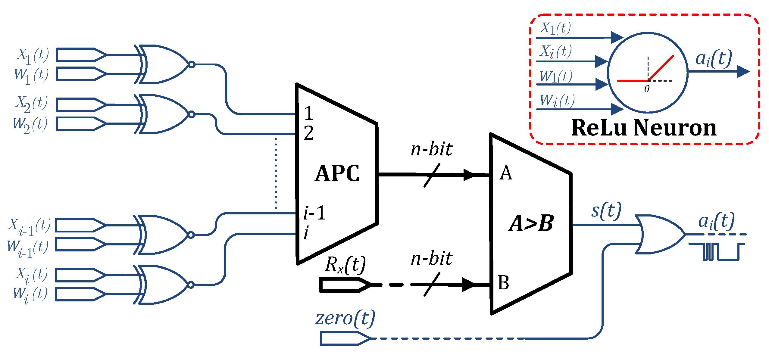
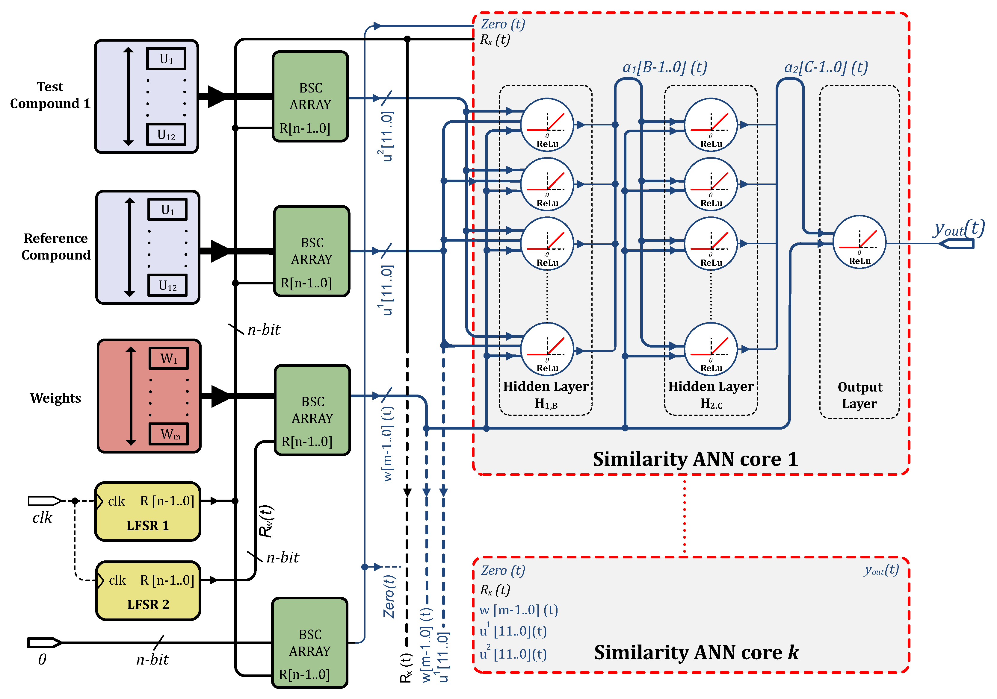
2.4. Stochastic Computing Neuron

To implement a SC artificial neuron, we propose the circuit shown in Figure 6. The input vector $\mathbf{x}\left(t\right)$ is multiplied by the weight vector $\mathbf{w}\left(t\right)$ through an array of XNOR gates, in a similar way to other neural approaches found in the literature [37]. Addition is carried out by an accumulative parallel counter (APC) [52]. The APC estimates the number of high values minus the number of low values from the i inputs during a total of N clock cycles. The APC circuit outputs a two’s complement value, which represents an estimation of the scalar product between $\mathbf{x}\left(t\right)$ and $\mathbf{w}\left(t\right)$. The advantage of using an APC instead of other SC addition circuits, such as a MUX or an OR gate, is that the APC is a correlation-independent circuit [53]. This makes the correlation introduced by the XNOR gates in the multiplication isolated, giving exact results after the addition. Once the addition is performed, we need to convert it again to the stochastic domain to continue operating in the following layers. For this purpose, a binary to stochastic converter is used, obtaining the APC stochastic signal $s\left(t\right)$, as seen in Figure 6.

The transfer function (SC-ReLU) is implemented by exploiting correlation between signals. Following the rules expressed in Equation (4), the $max$ function can be implemented with a single OR gate in the stochastic domain if the input signals are totally correlated ($C(s,zero)=1$). For this reason, to implement the SC-ReLU in the neuron, the signals $s\left(t\right)$ and $zero\left(t\right)$ are generated by using the same RNG ($R_x\left(t\right)$). The signal $zero\left(t\right)$ is a bit stream which contains 50% of ones, thus representing a zero bipolar number. The stochastic output activation $a\left(t\right)$ is, therefore,

$$a\left(t\right)=max\left(\sum _{q=1}^i{x}_q\left(t\right){\omega }_q\left(t\right),0\right)$$

(5)

The SC-ReLU design of this work is in high contrast with those ones found in the SC literature. A. Ren et al. [53] presented a SC-ReLU design based on segment slicing. This was carried out by using high-cost digital counters for each input argument, entailing an increase in footprint area (see Figure 8 in the original paper [53]). J. Yu et al. provided another approach to implement SC-ReLUs [54]. That design was based on an FSM circuit, which depends on its state to set the stochastic output (see Figure 5a in the original paper [54]). Z. Li et al. [55] used a circuit based on counters and accumulators, clipping the ReLU output to one (see Figure 6 in the original paper [55]). None of these SC-ReLU designs takes advantage of the correlation phenomenon, and they are also not area efficient. Moreover, all these approaches suggested by the literature do not have any control over the correlation level of the outcome, being unpredictable. This is a problem for the following layers for which full decorrelation must be guaranteed in order to perform the multiplication operation. If not guaranteed, it leads to accumulating inaccuracies when the signal goes to the next layer. By contrast, in the approach we propose, the correlation is intentionally manipulated to exploit the best of the two worlds (correlation and decorrelation), producing precise results, while saving plenty of resources.

2.5. Stochastic Computing ANN

Figure 7 shows a general view of the hardware implementation of the proposed VS hardware. As it can be observed, only two RNGs are needed for the whole VS acceleration system (LFSR1 and LFSR2 in the figure). The proposed architecture saves a large amount of hardware resources since RNG circuits are one of the most area-demanding blocks in stochastic computing designs. A linear feedback shift register (LFSR) circuit is used as a pseudo-RNG. The LFSR1 block generates $R_x\left(t\right)$, which is used in the stochastic conversion of the inputs ${\mathbf{u}}^{1,2}$, the zero reference signal and the APC binary output of each stochastic neuron. All these signals present maximum correlation. Binary to stochastic blocks ($BSC$) are employed to convert from the two’s complement to the stochastic domain, using LFSR sequences. The output vector of each layer is denoted as ${\mathbf{a}}_l$, where l stands for the hidden layer of the network. To attain total decorrelation between neuron inputs and weights (needed for multiplication), LFSR2 is employed as a second pseudo-RNG. It provides the signal $R_w\left(t\right)$) which generates the stochastic weight vector $\mathbf{w}\left(t\right)$.

As noted, the proposed stochastic hardware implementation exploits the correlation phenomenon between signals and, at the same time, minimizes the area usage by reducing the number of RNG employed in the circuit to only two LFSR blocks. Furthermore, the compounds’ stochastic signals ${\mathbf{u}}^1$ and the stochastic weights $\mathbf{w}\left(t\right)$ are shared by the k different cores (see dashed lines), thus allowing to increase parallelism. The hardware proposal can be embedded on a single chip, thus increasing the acceleration factor that this architecture can attain.

3. Results

3.1. Experimental Methodology

To evaluate the performance and capabilities of the proposed VS hardware, we used the DUD-E [45] database. This database contains 22,886 active compounds and their affinities to 102 targets.

We built the training set by incorporating 50% of actives and 10% of decoys from each target. Each sample of the training set incorporates two compounds as inputs: the crystal ligand of the target (${\mathbf{u}}^1$) and an active or a decoy for ${\mathbf{u}}^2$. We used a total of 162,530 samples for the training set and 1,300,804 ones for the testing set. A learning rate of $0.001$ with an Adam optimizer [56] was employed to train each model.

We performed our analysis based on two comparisons. First, we evaluated three different SC-ANN models and compared them with their software counterparts. Second, we compared the SC-ANN implementations with other ligand-based works present in the literature. The metrics we chose for the performance evaluation were (a) accuracy measured with the area under the curve (AUC) of the receiver operating characteristic (ROC) curve, (b) processing speed in inferences per second, and (c) energy efficiency in terms of inferences obtained per Joule invested. The AUC value was calculated for each target and the mean value was reported. The power reported for the SC models was calculated by the Power Analyzer Tool incorporated in the Quartus environment. We took into consideration the worst case scenario for the signal toggle rate (50% of variation). We reported the total power calculated by the tool. We embedded the maximum possible number of ANN cores on the FPGA, occupying the maximum amount of logic resources on the device. This makes the power consumption for the SC implementations practically the same (see ANN cores and FPGA ALM(%) columns in

Table 1. Performance comparison between FPGA measurements and software simulations for several ANN architectures.

Model	AUC Mean	Speed (inf/s)	Power (W)	Energy Efficiency (inf/Joule)	ANN Cores	FPGA ALM (%)	FPGA DSP (%)	FPGA BRAM (%)	Clk Freq (MHz)
SC-12	0.62	3,205,128	21	152,625	105	340,305 (80%)	0 (0%)	0 (0%)	125
SC-24	0.71	1,373,626	21	65,411	45	329,715 (77%)	0 (0%)	0 (0%)	125
SC-48	0.78	549,451	21	26,164	18	309,909 (73%)	0 (0%)	0 (0%)	125
SW-12	0.66	43,573	95	459	1	-	-	-	-
SW-24	0.72	42,034	95	442	1	-	-	-	-
SW-48	0.79	37,397	95	394	1	-	-	-	-

for details). As for the software, we reported the thermal design power (TDP) of the processor specified by the manufacturer.

3.2. Hardware Measurements vs. Software Simulations

Table 1 compares the performance of SC and software (SW) implementations. The model name points out the number of neurons in the first hidden layer, being 12 for 24-12-6-1, 24 for 24-24-12-1, and 48 for 24-48-24-1 architectures. The SW results were produced through an Intel(R) Xeon(R) X5670 processor with a 64-bit floating-point precision running at 2.93 GHz. Concerning the SC implementation, we used the same weights derived from its SW counterpart. SC results were measured by using a Gidel PROC10A board, which contains an Intel Arria-10 10AX115H3F34I2SG FPGA. This device has 427,200 ALMs, built with TSMC’s 20 nm process technology, improving the performance in regard to previous FPGA versions. Moreover, it has a PCI Express (PCIe) 3.0 specification (Gen3) IP that allows a rapid communication interface. The package is a $35\times 35$ mm${}^2$ 1152-FCBGA. We ran the application at a clock frequency of 125 MHz. As for the programming, we used the Quartus Prime 19.1 multiplatform environment.

The bit precision for the SC implementation was 12 bits, running a sequence length of $N=2^{12}-1=4095$ cycles. We embedded as many SC-ANN cores as possible on the device for the different architectures (reported in the ANN cores column). The number of FPGA resources employed is also pointed out in the table.

As shown, SC models display an AUC degradation with respect to the SW implementation of 0.04, 0.01, and 0.01 for the 12, 24, and 48 architectures, respectively. Nevertheless, they work 74, 33, and 15 times faster than their SW counterparts. Even more, they are more energy efficient by factors of 333×, 148×, and 66×. Additionally, we measured the AUC for the 12-bit quantized models (not shown in the table), and observed that the SC implementation did not exhibit any accuracy degradation. We thus conclude that the only degradation presented with respect to the SW results is because of the quantization process and not due to the stochasticity of the technique.

As it can be observed, no DSP or RAM are employed in the FPGA because a non-conventional approach is used for the calculus (SC), using only the distributed resources of the device. This fact undoubtedly shows the advantages provided by SC.

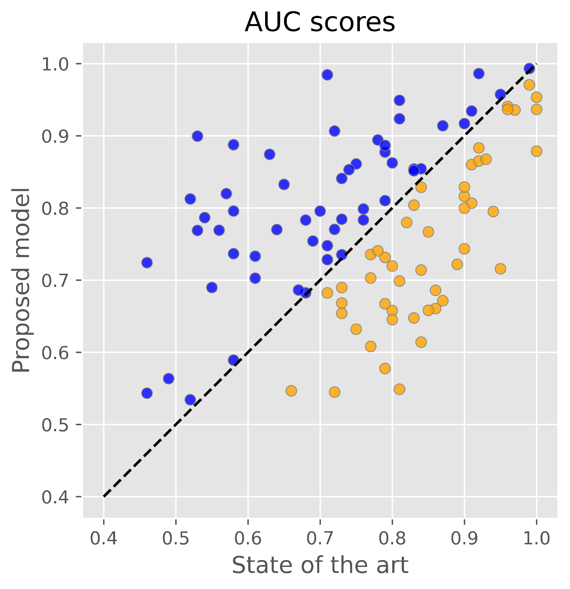
3.3. Comparison with Other Ligand-Based Models

Table 2. Performance comparison between this work and different ligand-based methods taken from the literature.

Model	AUC Mean	Speed (inf/s)
This work (SC-48)	0.78	549,451
This work (SC-24)	0.71	1,373,626
eSim-pscreen [57]	0.76	12.3
eSim-pfast [57]	0.74	61.2
eSim-pfastf [57]	0.71	274.9
mRAISE [58]	0.74	–
ROCS [59]	0.60	1820
USR [59,60]	0.52	$\mathbf{5}.\mathbf{0}\times {\mathbf{10}}^{\mathbf{6}}$
VAMS [59]	0.56	109,000
WEGA [61]	0.564	$1.6\times {10}^{-3}$
OptimPharm [61]	0.56	$8.7\times {10}^{-4}$

compares the SC models of this work with nine different ligand-based methods from the literature: eSim-pscreen [57], eSim-pfast [57], eSim-pfastf [57], mRAISE [58], ROCS [59], USR [59,60], VAMS [59], WEGA [61] and OptimPharm [61]. SC-48 outperforms all other methods in terms of AUC. It has an improvement of $0.02$ with respect to the best AUC ($0.76$) method of other works (eSim-pscreen [57]). What is more, it is 44,670 times faster. If we compare the SC-24 method with the fastest model in the literature (USR [59,60]), our proposal is 3.65 times slower, but it yields 0.19 more AUC.

A detailed analysis of the AUC for each individual target (from 102 in total) of the most accurate models in the literature is presented in

Table 3. Comparison of percentages linked to the different methods that fit a specific AUC threshold.

Model	% AUC <0.5	% AUC ≥0.6	% AUC ≥0.7	% AUC ≥0.8	% AUC ≥0.9
This work (SC-48)	0	92	74	43	18
eSim-pscreen [57]	5	81	69	43	17
eSim-pfast [57]	9	82	62	34	14
eSim-pfast [57]	5	79	53	26	6

. Each column presents, for each model, the percentage of targets that fits a specific AUC threshold. The proposed model presents the best results in the table (written in bold).

Table 4. Per target comparison of the current SC implementation versus state-of-the-art models. Data taken from [57].

Target	Proposed Model	Max (Other)	Target	Proposed Model	Max (Other)	Target	Proposed Model	Max (Other)
aa2ar	0.80	0.76	fabp4	0.85	0.83	mmp13	0.91	0.72
abl1	0.69	0.73	fak1	0.72	0.95	mp2k1	0.87	0.63
ace	0.86	0.75	fgfr1	0.98	0.71	nos1	0.90	0.53
aces	0.81	0.52	fkb1a	0.77	0.72	nram	0.83	0.9
ada	0.81	0.91	fnta	0.74	0.78	pa2ga	0.85	0.74
ada17	0.86	0.8	fpps	0.99	0.99	parp1	0.74	0.9
adrb1	0.80	0.7	gcr	0.77	0.64	pde5a	0.74	0.73
adrb2	0.83	0.65	glcm	0.89	0.78	pgh1	0.65	0.73
akt1	0.74	0.58	gria2	0.68	0.68	pgh2	0.85	0.84
akt2	0.55	0.66	grik1	0.67	0.73	plk1	0.78	0.82
aldr	0.75	0.71	hdac2	0.77	0.53	pnph	0.86	0.92
ampc	0.78	0.76	hdac8	0.77	0.85	ppara	0.92	0.9
andr	0.68	0.71	hivint	0.56	0.49	ppard	0.92	0.81
aofb	0.54	0.46	hivpr	0.83	0.84	pparg	0.89	0.79
bace1	0.79	0.54	hivrt	0.73	0.71	prgr	0.70	0.81
braf	0.74	0.77	hmdh	0.86	0.91	ptn1	0.82	0.57
cah2	0.99	0.92	hs90a	0.65	0.8	pur2	0.95	1
casp3	0.89	0.58	hxk4	0.82	0.9	pygm	0.80	0.58
cdk2	0.72	0.8	igf1r	0.73	0.61	pyrd	0.80	0.9
comt	0.97	0.99	inha	0.54	0.72	reni	0.81	0.79
cp2c9	0.53	0.52	ital	0.70	0.77	rock1	0.58	0.79
cp3a4	0.59	0.58	jak2	0.55	0.81	rxra	0.87	0.93
csf1r	0.66	0.8	kif11	0.65	0.83	sahh	0.94	1
cxcr4	0.73	0.79	kit	0.75	0.69	src	0.69	0.67
def	0.66	0.86	kith	0.93	0.91	tgfr1	0.71	0.84
dhi1	0.78	0.68	kpcb	0.66	0.85	thb	0.72	0.89
dpp4	0.78	0.73	lck	0.69	0.55	thrb	0.85	0.83
drd3	0.72	0.46	lkha4	0.61	0.84	try1	0.91	0.87
dyr	0.96	0.95	mapk2	0.69	0.86	tryb1	0.80	0.83
egfr	0.61	0.77	mcr	0.88	0.79	tysy	0.88	0.92
esr1	0.94	0.96	met	0.67	0.87	urok	0.95	0.81
esr2	0.94	0.97	mk01	0.67	0.79	vgfr2	0.63	0.75
fa10	0.84	0.73	mk10	0.77	0.56	wee1	0.88	1
fa7	0.94	0.96	mk14	0.70	0.61	xiap	0.79	0.94

shows a per target AUC score comparison between the SC-48 implementation and the best model of [57,58,59,61]. Figure 8 shows a graphical representation of this data. We can appreciate that the proposed model provides the best AUC score values for 53 of the targets present in the database.

4. Conclusions

This work shows the potential application of MPE descriptors and artificial neural networks (ANN) to virtual screening (VS). We have also shown a new methodology to accelerate the proposed VS process in an energy-efficient way by using stochastic computing (SC) hardware design techniques. An FPGA-compatible implementation is realized, and its performance in terms of accuracy, processing speed and energy efficiency is estimated. Compared to the state-of-the-art, the proposed model shows an increase by a factor of 44,670 in terms of processing speed and an improvement of 2% in terms of overall accuracy. We have also demonstrated the benefits attained by employing non-conventional (SC) hardware accelerators for ANN when processing huge databases. In particular, we have introduced a new methodology in which the implementation of the activation (ReLU) function exploits the correlation between signals, obtained thanks to the APC isolating characteristics. Overall, only two LFSR blocks are needed for the full ANN design in such a way that the impact of these blocks, historically regarded as the main drawback of SC, is minimized. To summarize, this work demonstrates the potential benefits of using non-conventional (stochastic) accelerators for ANNs when processing huge databases, especially suitable for those computationally costly processing problems, such as virtual screening.

References

1. Hoffmann, T.; Gastreich, M. The next level in chemical space navigation: Going far beyond enumerable compound libraries. Drug Discov. Today 2019, 24, 1148–1156. [Google Scholar] [CrossRef]
2. Adeshina, Y.O.; Deeds, E.J.; Karanicolas, J. Machine learning classification can reduce false positives in structure-based virtual screening. Proc. Natl. Acad. Sci. USA 2020, 117, 18477–18488. [Google Scholar] [CrossRef] [PubMed]
3. Fresnais, L.; Ballester, P.J. The impact of compound library size on the performance of scoring functions for structure-based virtual screening. Brief. Bioinform. 2020, 22, bbaa095. [Google Scholar] [CrossRef]
4. Lavecchia, A.; Giovanni, C. Virtual screening strategies in drug discovery: A critical review. Curr. Med. Chem. 2013, 20, 2839–2860. [Google Scholar] [CrossRef] [PubMed]
5. Singh, N.; Chaput, L.; Villoutreix, B. Virtual screening web servers: Designing chemical probes and drug candidates in the cyberspace. Brief. Bioinform. 2021, 22, 1790–1818. [Google Scholar] [CrossRef] [PubMed] [Green Version]
6. Glaab, E. Building a virtual ligand screening pipeline using free software: A survey. Brief. Bioinform. 2016, 17, 352–366. [Google Scholar] [CrossRef] [Green Version]
7. Ghislat, G.; Rahman, T.; Ballester, P.J. Recent progress on the prospective application of machine learning to structure-based virtual screening. Curr. Opin. Chem. Biol. 2021, 65, 28–34. [Google Scholar] [CrossRef]
8. Li, H.; Sze, K.H.; Lu, G.; Ballester, P. Machine-learning scoring functions for structure-based virtual screening. Compu. Mol. Sci. 2021, 11, e1478. [Google Scholar] [CrossRef]
9. Batool, M.; Ahmad, B.; Choi, S. A structure-based drug discovery paradigm. Int. J. Mol. Sci. 2019, 20, 2783. [Google Scholar] [CrossRef] [Green Version]
10. Pinzi, L.; Rastelli, G. Molecular docking: Shifting paradigms in drug discovery. Int. J. Mol. Sci. 2019, 20, 4331. [Google Scholar] [CrossRef] [Green Version]
11. Zoete, V.; Daina, A.; Bovigny, C.; Michielin, O. SwissSimilarity: A Web Tool for Low to Ultra High Throughput Ligand-Based Virtual Screening. J. Chem. Inf. Model. 2016, 56, 1399–1404. [Google Scholar] [CrossRef]
12. Li, H.; Leung, K.S.; Wong, M.H.; Ballester, P. USR-VS: A web server for large-scale prospective virtual screening using ultrafast shape recognition techniques. Nucleic Acids Res. 2016, 44, W436–W441. [Google Scholar] [CrossRef]
13. Kumar, A.; Zhang, K. Advances in the development of shape similarity methods and their application in drug discovery. Front. Chem. 2018, 6, 315. [Google Scholar] [CrossRef] [PubMed]
14. Neves, B.; Braga, R.; Melo-Filho, C.; Moreira-Filho, J.; Muratov, E.; Andrade, C. QSAR-based virtual screening: Advances and applications in drug discovery. Front. Pharmacol. 2018, 9, 1275. [Google Scholar] [CrossRef] [PubMed] [Green Version]
15. Soufan, O.; Ba-Alawi, W.; Magana-Mora, A.; Essack, M.; Bajic, V. DPubChem: A web tool for QSAR modeling and high-throughput virtual screening. Sci. Rep. 2018, 8, 9110. [Google Scholar] [CrossRef] [PubMed]
16. Speck-Planche, A.; Kleandrova, V.; Luan, F.; Cordeiro, M. Chemoinformatics in anti-cancer chemotherapy: Multi-target QSAR model for the in silico discovery of anti-breast cancer agents. Eur. J. Pharm. Sci. 2012, 47, 273–279. [Google Scholar] [CrossRef]
17. Olier, I.; Sadawi, N.; Bickerton, G.; Vanschoren, J.; Grosan, C.; Soldatova, L.; King, R. Meta-QSAR: A large-scale application of meta-learning to drug design and discovery. Mach. Learn. 2018, 107, 285–311. [Google Scholar] [CrossRef] [Green Version]
18. Sidorov, P.; Naulaerts, S.; Ariey-Bonnet, J.; Pasquier, E.; Ballester, P.J. Predicting Synergism of Cancer Drug Combinations Using NCI-ALMANAC Data. Front. Chem. 2019, 7, 509. [Google Scholar] [CrossRef]
19. Lavecchia, A. Machine-learning approaches in drug discovery: Methods and applications. Drug Discov. Today 2015, 20, 318–331. [Google Scholar] [CrossRef] [Green Version]
20. Azghadi, M.; Linares-Barranco, B.; Abbott, D.; Leong, P. A Hybrid CMOS-Memristor Neuromorphic Synapse. IEEE Trans. Biomed. Circuits Syst. 2017, 11, 434–445. [Google Scholar] [CrossRef] [Green Version]
21. Frenkel, C.; Legat, J.D.; Bol, D. MorphIC: A 65-nm 738k-Synapse/mm2 Quad-Core Binary-Weight Digital Neuromorphic Processor with Stochastic Spike-Driven Online Learning. IEEE Trans. Biomed. Circuits Syst. 2019, 13, 999–1010. [Google Scholar] [CrossRef] [Green Version]
22. Guo, W.; Yantır, H.; Fouda, M.; Eltawil, A.; Salama, K. Towards efficient neuromorphic hardware: Unsupervised adaptive neuron pruning. Electronics 2020, 9, 1059. [Google Scholar] [CrossRef]
23. Son, H.; Cho, H.; Lee, J.; Bae, S.; Kim, B.; Park, H.J.; Sim, J.Y. A Multilayer-Learning Current-Mode Neuromorphic System with Analog-Error Compensation. IEEE Trans. Biomed. Circuits Syst. 2019, 13, 986–998. [Google Scholar] [CrossRef] [PubMed]
24. Kang, M.; Lee, Y.; Park, M. Energy efficiency of machine learning in embedded systems using neuromorphic hardware. Electronics 2020, 9, 1069. [Google Scholar] [CrossRef]
25. Morro, A.; Canals, V.; Oliver, A.; Alomar, M.; Galan-Prado, F.; Ballester, P.; Rossello, J. A Stochastic Spiking Neural Network for Virtual Screening. IEEE Trans. Neural Netw. Learn. Syst. 2018, 29, 1371–1375. [Google Scholar] [CrossRef] [PubMed]
26. Nascimento, I.; Jardim, R.; Morgado-Dias, F. A new solution to the hyperbolic tangent implementation in hardware: Polynomial modeling of the fractional exponential part. Neural Comput. Appl. 2013, 23, 363–369. [Google Scholar] [CrossRef]
27. Carrasco-Robles, M.; Serrano, L. Accurate differential tanh(nx) implementation. Int. J. Circuit Theory Appl. 2009, 37, 613–629. [Google Scholar] [CrossRef]
28. Liu, B.; Zou, D.; Feng, L.; Feng, S.; Fu, P.; Li, J. An FPGA-based CNN accelerator integrating depthwise separable convolution. Electronics 2019, 8, 281. [Google Scholar] [CrossRef] [Green Version]
29. Zhang, M.; Li, L.; Wang, H.; Liu, Y.; Qin, H.; Zhao, W. Optimized compression for implementing convolutional neural networks on FPGA. Electronics 2019, 8, 295. [Google Scholar] [CrossRef] [Green Version]
30. Gaines, B.R. Stochastic computing systems. In Advances in Information Systems Science; Springer: New York, NY, USA, 1969; pp. 37–172. [Google Scholar]
31. Alaghi, A.; Hayes, J. Survey of stochastic computing. Trans. Embed. Comput. Syst. 2013, 12, 1–19. [Google Scholar] [CrossRef]
32. Canals, V.; Morro, A.; Rosselló, J. Stochastic-based pattern-recognition analysis. Pattern Recognit. Lett. 2010, 31, 2353–2356. [Google Scholar] [CrossRef] [Green Version]
33. Faix, M.; Laurent, R.; Bessiere, P.; Mazer, E.; Droulez, J. Design of stochastic machines dedicated to approximate Bayesian inferences. IEEE Trans. Emerg. Top. Comput. 2019, 7, 60–66. [Google Scholar] [CrossRef] [Green Version]
34. Joe, H.; Kim, Y. Novel stochastic computing for energy-efficient image processors. Electronics 2019, 8, 720. [Google Scholar] [CrossRef] [Green Version]
35. Alaghi, A.; Li, C.; Hayes, J. Stochastic circuits for real-time image-processing applications. In Proceedings of the 50th Annual Design Automation Conference, Austin, TX, USA, 2–6 June 2013. [Google Scholar]
36. Xiao, S.; Liu, W.; Guo, Y.; Yu, Z. Low-Cost Adaptive Exponential Integrate-and-Fire Neuron Using Stochastic Computing. IEEE Trans. Biomed. Circuits Syst. 2020, 14, 942–950. [Google Scholar] [CrossRef] [PubMed]
37. Rosselló, J.L.; Canals, V.; Morro, A. Hardware implementation of stochastic-based Neural Networks. In Proceedings of the 2010 International Joint Conference on Neural Networks (IJCNN), Barcelona, Spain, 18–23 July 2010; pp. 1–4. [Google Scholar] [CrossRef]
38. Tomlinson, M.S., Jr.; Walker, D.; Sivilotti, M. A digital neural network architecture for VLSI. In Proceedings of the 1990 IJCNN International Joint Conference on Neural Networks, San Diego, CA, USA, 17–21 June 1990; Volume 2, pp. 545–550. [Google Scholar] [CrossRef]
39. Moon, G.; Zaghloul, M.; Newcomb, R. VLSI implementation of synaptic weighting and summing in pulse coded neural-type cells. IEEE Trans. Neural Netw. 1992, 3, 394–403. [Google Scholar] [CrossRef]
40. Sato, S.; Yumine, M.; Yama, T.; Murota, J.; Nakajima, K.; Sawada, Y. LSI implementation of pulse-output neural network with programmable synapse. In Proceedings of the [Proceedings 1992] IJCNN International Joint Conference on Neural Networks, Baltimore, MD, USA, 7–11 June 1992; Volume 1, pp. 172–177. [Google Scholar] [CrossRef]
41. Yousefzadeh, A.; Stromatias, E.; Soto, M.; Serrano-Gotarredona, T.; Linares-Barranco, B. On Practical Issues for Stochastic STDP Hardware with 1-bit Synaptic Weights. Front. Neurosci. 2018, 12, 665. [Google Scholar] [CrossRef] [Green Version]
42. Fox, S.; Faraone, J.; Boland, D.; Vissers, K.; Leong, P.H. Training Deep Neural Networks in Low-Precision with High Accuracy Using FPGAs. In Proceedings of the 2019 International Conference on Field-Programmable Technology (ICFPT), Tianjin, China, 9–13 December 2019; pp. 1–9. [Google Scholar] [CrossRef]
43. Ichihara, H.; Ishii, S.; Sunamori, D.; Iwagaki, T.; Inoue, T. Compact and accurate stochastic circuits with shared random number sources. In Proceedings of the 2014 IEEE 32nd International Conference on Computer Design (ICCD), Seoul, Korea, 19–22 October 2014; pp. 361–366. [Google Scholar] [CrossRef]
44. Oliver, A.; Canals, V.; Rosselló, J. A Bayesian target predictor method based on molecular pairing energies estimation. Sci. Rep. 2017, 7, 43738. [Google Scholar] [CrossRef] [Green Version]
45. Mysinger, M.; Carchia, M.; Irwin, J.; Shoichet, B. Directory of useful decoys, enhanced (DUD-E): Better ligands and decoys for better benchmarking. J. Med. Chem. 2012, 55, 6582–6594. [Google Scholar] [CrossRef]
46. Sliwoski, G.; Kothiwale, S.; Meiler, J.; Lowe, E., Jr. Computational methods in drug discovery. Pharmacol. Rev. 2014, 66, 334–395. [Google Scholar] [CrossRef] [Green Version]
47. Gasteiger, J.; Marsili, M. Iterative partial equalization of orbital electronegativity—A rapid access to atomic charges. Tetrahedron 1980, 36, 3219–3228. [Google Scholar] [CrossRef]
48. Halgren, T. Merck molecular force field. I. Basis, form, scope, parameterization, and performance of MMFF94. J. Comput. Chem. 1996, 17, 490–519. [Google Scholar] [CrossRef]
49. Nair, V.; Hinton, G.E. Rectified linear units improve restricted boltzmann machines. In Proceedings of the 27th International Conference on Machine Learning, Haifa, Israel, 21–24 June 2010. [Google Scholar]
50. Gaines, B.R. Origins of Stochastic Computing. In Stochastic Computing: Techniques and Applications; Springer International Publishing: Cham, Switzerland, 2019; pp. 13–37. [Google Scholar]
51. Alaghi, A.; Hayes, J. Exploiting correlation in stochastic circuit design. In Proceedings of the 2013 IEEE 31st International Conference on Computer Design (ICCD), Asheville, NC, USA, 6–9 October 2013. [Google Scholar]
52. Parhami, B.; Chi-Hsiang, Y. Accumulative parallel counters. In Proceedings of the Conference Record of The Twenty-Ninth Asilomar Conference on Signals, Systems and Computers, Pacific Grove, CA, USA, 30 October–2 November 1995; Volume 2, pp. 966–970. [Google Scholar] [CrossRef]
53. Ren, A.; Li, Z.; Ding, C.; Qiu, Q.; Wang, Y.; Li, J.; Qian, X.; Yuan, B. Sc-dcnn: Highly-scalable deep convolutional neural network using stochastic computing. ACM SIGPLAN Not. 2017, 52, 405–418. [Google Scholar] [CrossRef]
54. Yu, J.; Kim, K.; Lee, J.; Choi, K. Accurate and efficient stochastic computing hardware for convolutional neural networks. In Proceedings of the 2017 IEEE International Conference on Computer Design (ICCD), Boston, MA, USA, 5–8 November 2017; pp. 105–112. [Google Scholar]
55. Li, Z.; Li, J.; Ren, A.; Cai, R.; Ding, C.; Qian, X.; Draper, J.; Yuan, B.; Tang, J.; Qiu, Q.; et al. HEIF: Highly efficient stochastic computing-based inference framework for deep neural networks. IEEE Trans. Comput.-Aided Des. Integr. Circuits Syst. 2018, 38, 1543–1556. [Google Scholar] [CrossRef]
56. Yaguchi, A.; Suzuki, T.; Asano, W.; Nitta, S.; Sakata, Y.; Tanizawa, A. Adam Induces Implicit Weight Sparsity in Rectifier Neural Networks. In Proceedings of the 2018 17th IEEE International Conference on Machine Learning and Applications (ICMLA), Orlando, FL, USA, 17–20 December 2018; pp. 318–325. [Google Scholar] [CrossRef] [Green Version]
57. Cleves, A.; Johnson, S.; Jain, A. Electrostatic-field and surface-shape similarity for virtual screening and pose prediction. J. Comput.-Aided Mol. Des. 2019, 33, 865–886. [Google Scholar] [CrossRef] [PubMed] [Green Version]
58. Von Behren, M.; Rarey, M. Ligand-based virtual screening under partial shape constraints. J. Comput.-Aided Mol. Des. 2017, 31, 335–347. [Google Scholar] [CrossRef] [PubMed]
59. Koes, D.R.; Camacho, C.J. Shape-based virtual screening with volumetric aligned molecular shapes. J. Comput. Chem. 2014, 35, 1824–1834. [Google Scholar] [CrossRef] [PubMed] [Green Version]
60. Ballester, P.J.; Richards, W.G. Ultrafast shape recognition to search compound databases for similar molecular shapes. J. Comput. Chem. 2007, 28, 1711–1723. [Google Scholar] [CrossRef] [PubMed]
61. Puertas-Martín, S.; Redondo, J.L.; Ortigosa, P.M.; Pérez-Sánchez, H. OptiPharm: An evolutionary algorithm to compare shape similarity. Sci. Rep. 2019, 9, 1398. [Google Scholar] [CrossRef] [Green Version]
Figure 1. The process of similarity comparison between a set of query compounds with unknown chemical properties and a compound with known activity against a specific therapeutic target.
Electronics 10 02981 g001
Figure 2. Clustering capacity of pairing-energy descriptors when using the most negative and most positive MPE values for five different DUD-E targets.
Electronics 10 02981 g002
Figure 3. ANN architecture employed for the estimation of similarity between two compounds. Each compound u j k is described by 12 energy descriptors, where j is the j t h component of the k t h compound, H l , j stands for the j t h neuron in the l t h hidden layer; B and C are the number of neurons in the first and the second hidden layer; and y o u t is the prediction of the model.
Electronics 10 02981 g003
Figure 4. Example of a SC bipolar multiplier. Two switching inputs x and y represent signals 0 and 0.5 , respectively. Afterward, they are multiplied through the XNOR gate, leading to signal z = 0.0 . Signal y ( t ) is generated with an independent RNG (not shown in the picture). Stochastic signals are colored in blue.
Electronics 10 02981 g004
Figure 5. Correlation between signals can change the function implemented by logic gates. Stochastic signals x ( t ) and y ( t ) are said to be perfectly correlated when they share the same RNG R ( t ) . Stochastic signals are noted in blue.
Electronics 10 02981 g005
Figure 6. Stochastic neuron design exploits correlation to reduce area cost. The stochastic vectors x ( t ) and w ( t ) are uncorrelated, producing a stochastic multiplication with XNOR gates. Stochastic units are noted in blue, while the two’s complement signals are in black.
Electronics 10 02981 g006
Figure 7. Neural network implementation using two LFSRs for the whole system. LFSR1 is used to generate the input stochastic vector u 1 , 2 , the zero bipolar signal z e r o ( t ) and the APC outcome inside each neuron. LFSR2 is used to generate the weight stochastic vector w ( t ) . Shared signals among the k ANN cores are depicted in dashed lines. Signals with n-bit two’s complement are noted in black, whereas stochastic signals are noted in blue.
Electronics 10 02981 g007
Figure 8. Visual representation of the scores shown in Table 4. Dots in blue indicate that the proposed VS system performs better; otherwise, we highlight the dots in orange color.
Electronics 10 02981 g008