Muon–Electron Pulse Shape Discrimination for Water Cherenkov Detectors Based on FPGA/SoC

Abstract

The distinction of secondary particles in extensive air showers, specifically muons and electrons, is one of the requirements to perform a good measurement of the composition of primary cosmic rays. We describe two methods for pulse shape detection and discrimination of muons and electrons implemented on FPGA. One uses an artificial neural network (ANN) algorithm; the other exploits a correlation approach based on finite impulse response (FIR) filters. The novel hls4ml package is used to build the ANN inference model. Both methods were implemented and tested on Xilinx FPGA System on Chip (SoC) devices: ZU9EG Zynq UltraScale+ and ZC7Z020 Zynq. The data set used for the analysis was captured with a data acquisition system on an experimental site based on a water Cherenkov detector. A comparison of the accuracy of the detection, resources utilization and power consumption of both methods is presented. The results show an overall accuracy on particle discrimination of 96.62% for the ANN and 92.50% for the FIR-based correlation, with execution times of 848 ns and 752 ns, respectively.

1. Introduction

The use of water Cherenkov detectors (WCD) has recently become widespread in the cosmic ray experimental community due to their easy implementation and relatively low cost. The Pierre Auger Observatory in Malargüe, Argentine [1], HAWC in Sierra Negra, Mexico [2] and the Latin American Giant Observatory (LAGO) collaboration that spans in Latin America are some examples of experiments that use this type of detector. The data acquisition systems (DAQ) used in these detectors have improved in the last decade, with sampling frequencies moving from 40 MHz to 120 MHz [3]. This indicates that the next generation of acquisition systems will reach a sampling rate of 500 MHz or more, which will allow analysis based on the shape of the pulses and also a much greater amount of data to be stored. The real-time analysis system is a new tool that is being implemented that allows not only the evaluation of valid events for storage but also their classification.

Custom DAQ have been developed and upgraded in order to continuously improve the sampling rate and dynamic range of WCD detectors: starting from a 12-bit, 40 MHz board with a design based on Pierre Auger’s electronics (as presented in [4]), through a Red Pitaya [5] (XC7Z010) 14-bit on-board ADC at 125 MHz (like the one in [6]), up to a high-speed 8-bit 500 MHz ADC (as the one used by [7]). With no exception, these DAQ systems accomplish the same goal (with some improvements and added capabilities) of digitizing, storing and sending raw events data to a remote repository while receiving setup commands and self-calibrating their amplifiers’ baselines.

Cosmic rays (CRs) are groups of several particles traveling at relativistic speeds through extremely long distances within space. CRs were discovered at the beginning of the 20th century, and there is still no accepted model to completely describe their behavior. Their origin is not exactly known either, but in one hypothesis, it is recalled that supernovae may be one of the sources [8]. In a recent discovery, it was experimentally shown that CRs detected at Earth come from extragalactic sources, and the importance of determining their direction of arrival was demonstrated [9]. The energy spectra of the CRs determine whether they are classified as very high-energy or ultra-high-energy.

Gamma-ray bursts (GRBs) were discovered in the late 1960s and are composed solely of photons. Their uncertain origin is similar to that of CRs; they are also hypothetically sourced from supernovae. One of the key characteristics of the GRBs is their high directivity, making them hard to detect when not directly pointed at Earth [8].

Both CRs and GRBs are able to trigger detectors; thus, separation and consequently determination of the muon/electron particle ratio arriving at WCDs at ground level provides complementary information about the energy of the primary particle that triggered the event in the atmosphere. This is especially important in the study of ultra-high-energy cosmic rays whose energy spectrum above ${10}^{10}$ GeV is not yet well known [10]. The use of WCD has also been proposed for the study of GRBs [4], whose origins present one of the most exciting open problems in modern astrophysics [11].

In this work, two approaches for online discrimination between muons and electrons pulses in WCD on triggered events are presented. One method is based on finite impulse response (FIR) filters and the other on artificial neural network (ANN) algorithms. Both methods were implemented and tested on Xilinx FPGA System on Chip (SoC) devices: a ZU9EG Zynq UltraScale+ and a ZC7Z020 Zynq chips mounted on ZCU102 and Zedboard development boards, respectively. The data set used for the analysis was captured from a WCD sited in Guatemala City using a Red-Pitaya-based front-end to collect the raw signals. The data set was characterized offline for the test and delivered into our experimental setup using the embedded processor in the SoC by a direct memory access (DMA) link.

The main contributions of this paper may be summarized as follows:

• a SoC FPGA implementation of two methods for pulse shape analysis for cosmic rays detection with high overall accuracy and low execution times;
• a pulse shape discriminator through a neural network inference, getting a fast and accurate model, using compression techniques and reconfigurable hardware for computation acceleration;
• the use of the novel hls4ml package in the context of cosmic rays detection to map the inference stage into the FPGA;
• the use of a correlation method using FIR filters and the design of a decision logic for online pulse discrimination;
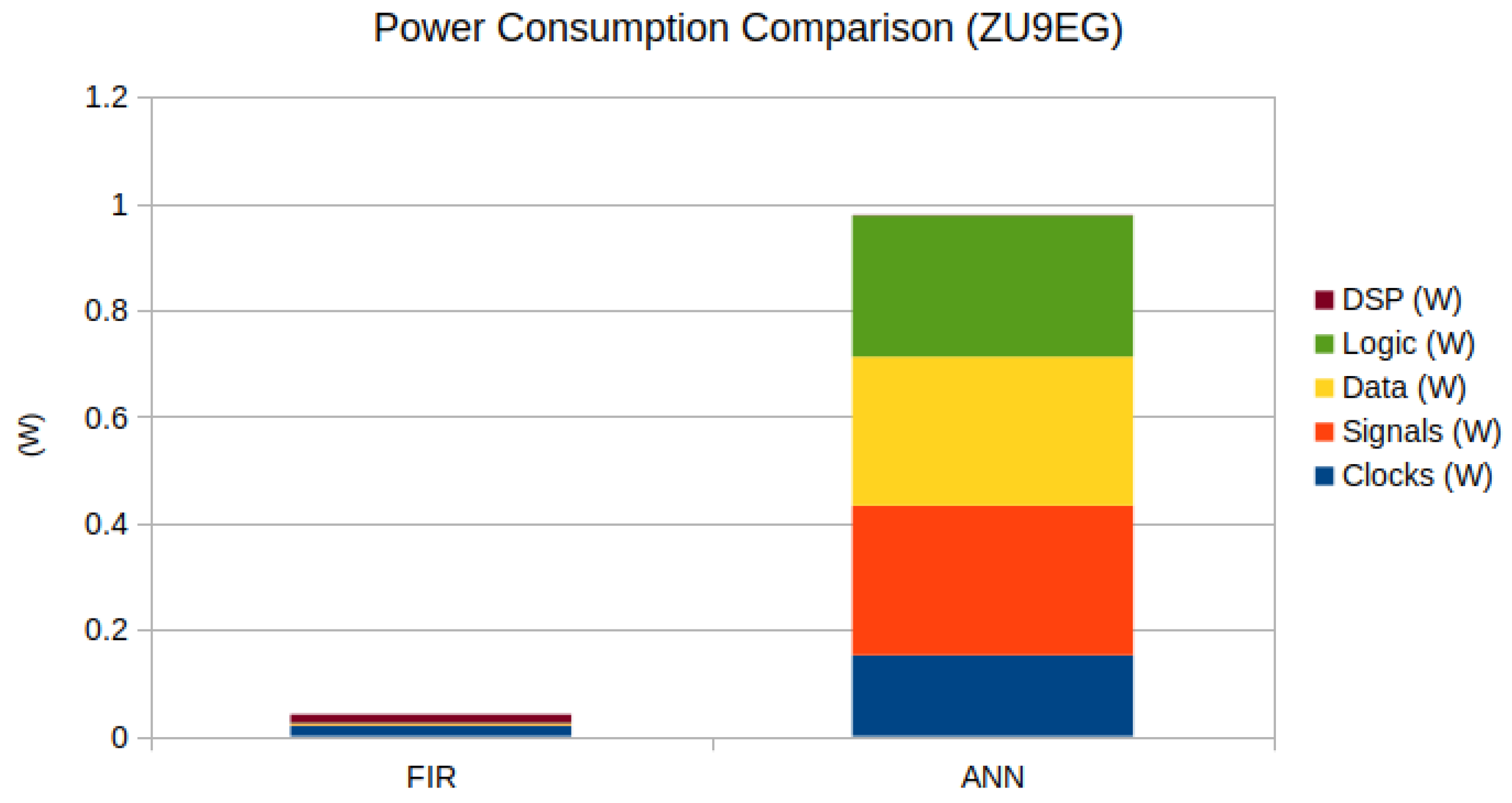
• a comparison of these methods in two different SoC FPGA platforms measuring resources utilization, power consumption and execution times.

The rest of the article is organized as follows: in Section 2, the related works and current approaches for cosmic ray discrimination using ANN and FIR is discussed. In Section 3, the data acquisition and analysis, selection criteria and the methodology of the design for both methods is described. In Section 4, the implementation on hardware for both methods as well as their partial results is presented. In Section 5, both methodologies are compared with an in-deep analysis of the overall accuracy, resource utilization, execution times and power consumption on each method. Conclusions and future work are presented in Section 6.

2. Related Works

Pulse shape discrimination (PSD) techniques are used in the context of particle detection to solve common classification problems when a digitized signal can be identified according to its features. With the development of new electronic devices, PSD methods have been implemented, within which stand out zero crossing, charge comparison, pulse gradient analysis (PGA), cross-correlation and neural network, among others [12,13,14,15].

A WCD produces pulses that contain information about the type of particle, energy and distance traveled that may be difficult to analyze using low-cost methods. Being able to classify these pulses based on their shape provides a way to access the information contained in them.

PSD has been proposed for other types of detectors [16,17,18] and also studied for WCDs [19]. Regarding muon–electron discrimination in WCDs, Salazar and Villasenor conducted a research study to measure properties of cosmic rays [20], including detection of decaying and crossing muons, an application of these results to calibrate WCD and a technique to separate isolated muons and electrons.

The main advantage of identifying the particles that originate the pulses is to be able to determine the muon–electron ratio since, in the case of observatories that monitor cosmic rays, this ratio is related to the particle that triggers the extensive air showers (EAS) [21].

The use of FPGAs and SoCs is a common practice in cosmic rays instrumentation [22], mostly in the front-end acquisition but also in basic data analysis and preprocessing. Complex analysis performed by software requires high computational cost and long execution times. With the development of new algorithms and technologies, FPGA can now compete with other high-performance computing processors due to their capability of parallel processing in online analysis and low power consumption per operation. Some of these methods are based on neural networks and FIR filters, as described in the following subsections.

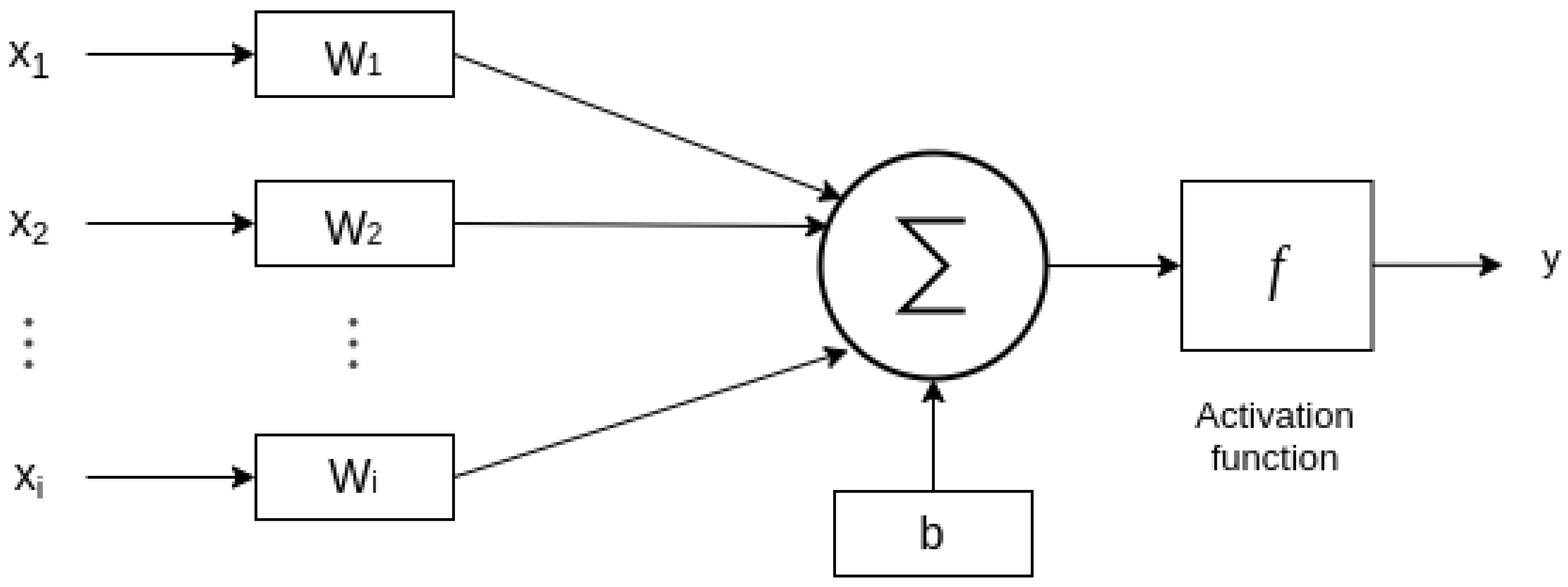
2.1. Neural Networks

Machine learning techniques have been used for offline pulse shape discrimination, obtaining high accuracy using floating-point precision. A fully connected layer architecture for PSD was presented in [23], obtaining an accuracy of 99.89%, managing to distinguish between good events from all noise/bad events. The work presented in [24] showed the efficient use of a convolutional neural network (CNN) for pulse discrimination, using raw SiPM signals as input, obtaining an accuracy of 0.995 ± 0.003. The network classifies electron and nuclear scintillation signals, and the results obtained with this approach were compared with charge integration and continuous wavelet transform methods, achieving an accuracy of 0.964 (±0.004) and 0.974 (±0.003), respectively. Holl et al. [25] implemented two stages for PSD in the context of germanium detectors using two neural network architectures trained in a separable manner: (1) an autoencoder CNN for feature extraction and their storage in low-dimensional vectors and (2) a network for classification based on fully connected layers. The work presented in [26] proposed the use of deep learning for electron identification with a simple binary classification task: a signal class (electrons) or a background class (protons). For this approach, two techniques were used: multivariate analysis using a multilayer perceptron and pattern recognition using CNN. The neural networks presented refine the cosmic electrons measurements by improving the background rejection at the highest.

The first attempt to use a neural network for a muon–electron pulse shape discriminator in WCD was presented in [27], where the authors employed Kohonen [28] topology to identify these classes of particles, obtaining an accuracy of 80%.

Numerous works aim to map neural networks inference into FPGAs, due to their features like reduced power consumption, high parallelism, high bandwidth and low latency, among others. An extended review in this topic can be found in [29]. Wei et al. [30] proposed a framework for deconvolutional neural networks (DCNN) hardware accelerators, focusing on the efficient utilization of the on-chip memory to improve the performance of the layers bounded by memory. The work presented in [31] proposed an FPGA architecture for DCNNs, and to optimize performance, the authors used loop unrolling and pipelining, memory partitioning and register insertion. Authors in [32] presented a hardware/software co-design for inference tasks; convolutional pooling and padding layers were implemented in FPGA, the rest of the layers were implemented into ARM processor and the computations were realized in reduced precision—8-bit magnitude and sign format.

NEURAghe [33] is a CNN accelerator which uses a soft processor to manage the execution of complex CNNs on the Zynq SoC. The hardware accelerator executes the convolutional layers, while the ARM cores are responsible for the execution of fully connected layers and data marshaling. The authors also proposed a complete and hardware-agnostic open-source software stack to enable an efficient implementation of CNN: the NEURAghe Deep Neural Network software stack (NeuDNN). hls4ml is a package developed by Duarte et al. [34] to achieve fast inference times in the context of high-energy physics. This tool maps the model obtained with Keras, PyTorch and TensorFlow, among others, to a Xilinx High-Level Synthesis project. The authors of [35] presented an FPGA implementation for trigger applications based on neural networks using VHDL to describe the convolutional network architecture.

From the literature review, we observed that it is feasible to implement a pulse shape discriminator using a neural network to obtain a fast and accurate model and, at the same time, translate the inference to describe the final hardware to be mapped into FPGA/SoC technology.

2.2. FIR Filters

Finite impulse response (FIR) filters are extensively used in digital signal processing (DSP) in cosmic rays detectors and can be easily implemented in reconfigurable platforms. There are several types of implementation on FPGAs ranging from the conventional tapped delay line implemented in Xilinx FIR Compiler [36] to distributed arithmetic filters [37]. This flexibility of implementation in hardware added to the freedom of choice of the coefficients opens the door for high-performance analysis and signal configuration in particle detectors.

Trapezoidal filters are often used for preprocessing to select pulses above an “event candidate” threshold in fluorescence detector arrays [38]. This type of application is used for a single feature extraction in case of a well-known type of signal. This allows fast rejection of noise in the input signal for later, typically slower postprocessing. Other applications like triangular filter algorithms (TFA) have also been used to discriminate between neutron and gamma events. However, according to Balmer [39], this method is still less efficient for pulse discrimination in ${}^{6}Li$ scintillators compared with two other computation-intensive methods: charge comparison method (CCM) and frequency gradient analysis (FGA). According to Balmer, CCM, which is the study of the entire pulse and the tail of the pulse to discriminate the event in small time windows, presents the best performance. The second best was FGA, which performs the analysis based on a fast Fourier transform (FFT) and is a variation using an FIR of a PGA that takes advantage of the difference between the peak and the sample amplitude of the pulses [15].

Some implementations, such as adaptive FIR filters, are used for linear prediction to reduce narrow band radio frequency interference in cosmic rays [40]. They improve the signal-to-noise ratio by calculating the covariance of the noise to identify undesired frequency components from external noise and later adapting the coefficients of the FIR filter in the front-end electronics. The authors calculated the covariance using the FPGA and later the microprocessor to calculate the new set of coefficients. The authors concluded that the linear predictor is a viable alternative to other methods such as digital notch filters or multiple time-to-frequency domain conversion using FFT.

For pulse shape analysis, where the signal is compared with different references, the joint variability of the signal with each reference must be normalized to be able to measure, by the magnitude of the result, the strength of the linear relation of the signal with reference. Using the precedent of using FIR for covariance implementation on FPGA, we can obtain the correlation by normalizing the coefficients by their standard deviation.

Correlation is used for pulse shape analysis, but it is often performed in postprocessing using software. This may be disadvantageous and lead to a high computational cost for single pulse analysis, which is challenging in embedded applications. Some implementations on FPGA are often utilized in cryptography [41] and neurological image analysis [42] where they take advantage of the parallelism to improve the performance. In the context of WCD, the reference signal for each type of particle is static, making it feasible to use a FIR with normalized coefficients to perform the correlation online. This will save time on postprocessing where millions of pulses need to be discriminated.

3. Methodology

3.1. Data Acquisition

The test platform is composed by a ground-based water Cherenkov gamma-ray burst detector, which features a Photonis XP1802 [43] photomultiplier tube (PMT) as the main sensor device [4,44,45,46]. An analog front-end (AFE) board sets the sensor’s high-voltage control input and provides a regulated power supply for the whole system. Finally, a slow-control implementation continuously monitors and computes the PMT baseline reference, according (but not limited) to the local temperature and atmospheric pressure measurements, which are also sampled on-board, as explained in [6]. A high-level block diagram of the used hardware is shown in Figure 1.

3.1.1. Analog Front-End

The AFE daughter board is directly attached to a Red Pitaya development board, similar to the one shown in [6]. This secondary AFE board contains an EMCO model C20 high-voltage DC-HVDC converter, configurable in a range between 0 VDC to 2000 VDC, at ∼1 V steps. The high-voltage output granularity is limited by the resolution of the (12-bit) digital-to-analog converter that sets the power supply’s input (control) voltage, as well as the supply’s regulation and ripple capabilities, specified in [47,48].

A coupling capacitor isolates the high-voltage signal (as done in [49,50]) from the sensor’s output signal, allowing the PMT to be connected to the low-voltage filtering and amplifying stage within the main board. By taking advantage of the ADC and antialias network integrated in the Red Pitaya board, only a 50 $\Omega$ terminator is added in parallel at the end of the coaxial cable that carries the signal from the PMT to the board, in order to match impedance. This signal is directly fed into the integrated ADC signal chain within the Red Pitaya, starting with the low-pass antialias filtering (with a −3 dB cutoff frequency of 50 MHz) and a 14-bit 125 MHz single-ended analog-to-digital converter.

3.1.2. Slow Control

In order to keep the signal span within the desired range and therefore achieve the expected signal resolution, any constant (DC) voltage component at the single-ended input should be mitigated [51]. However, the analog input stage integrated in the Red Pitaya board is not configurable, so it would be mandatory to add external circuitry to implement a traditional slow-control circuit [52] by dynamically setting the amplifiers’ baseline reference voltage. Therefore, a DSP technique is used instead, as done in [6], taking advantage of FPGA-specific resources, so LUT utilization is reduced and the inherent delay in the signal path is decreased [53]. Temperature and pressure compensation is also included in the embedded ARM processor algorithm, so no external hardware components are required between the PMT’s coupling capacitor and the main board’s analog input. A low cutoff frequency (sub-Hz) high-pass filter could be used to replace the slow-control mechanism implemented in the FPGA fabric at the cost of losing temperature and atmospheric pressure compensation, and also introducing a significant group delay and distortion of the original detected signal [54]. The latter approach may only be used if no amplitude information is mandatory (such as time-to-digital converter systems), where an analog voltage comparator discriminates values within an amplitude window and only timing data is preserved [55].

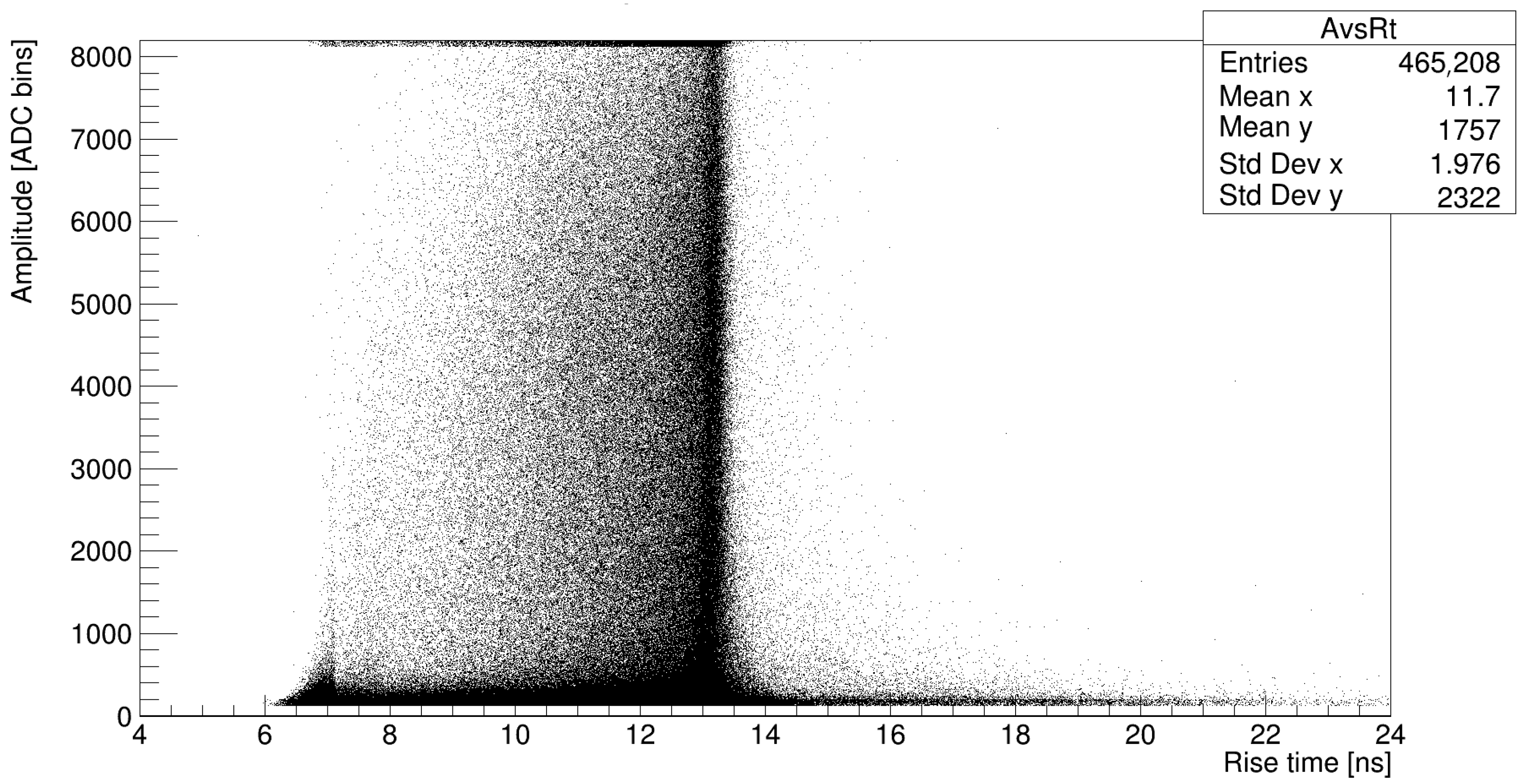
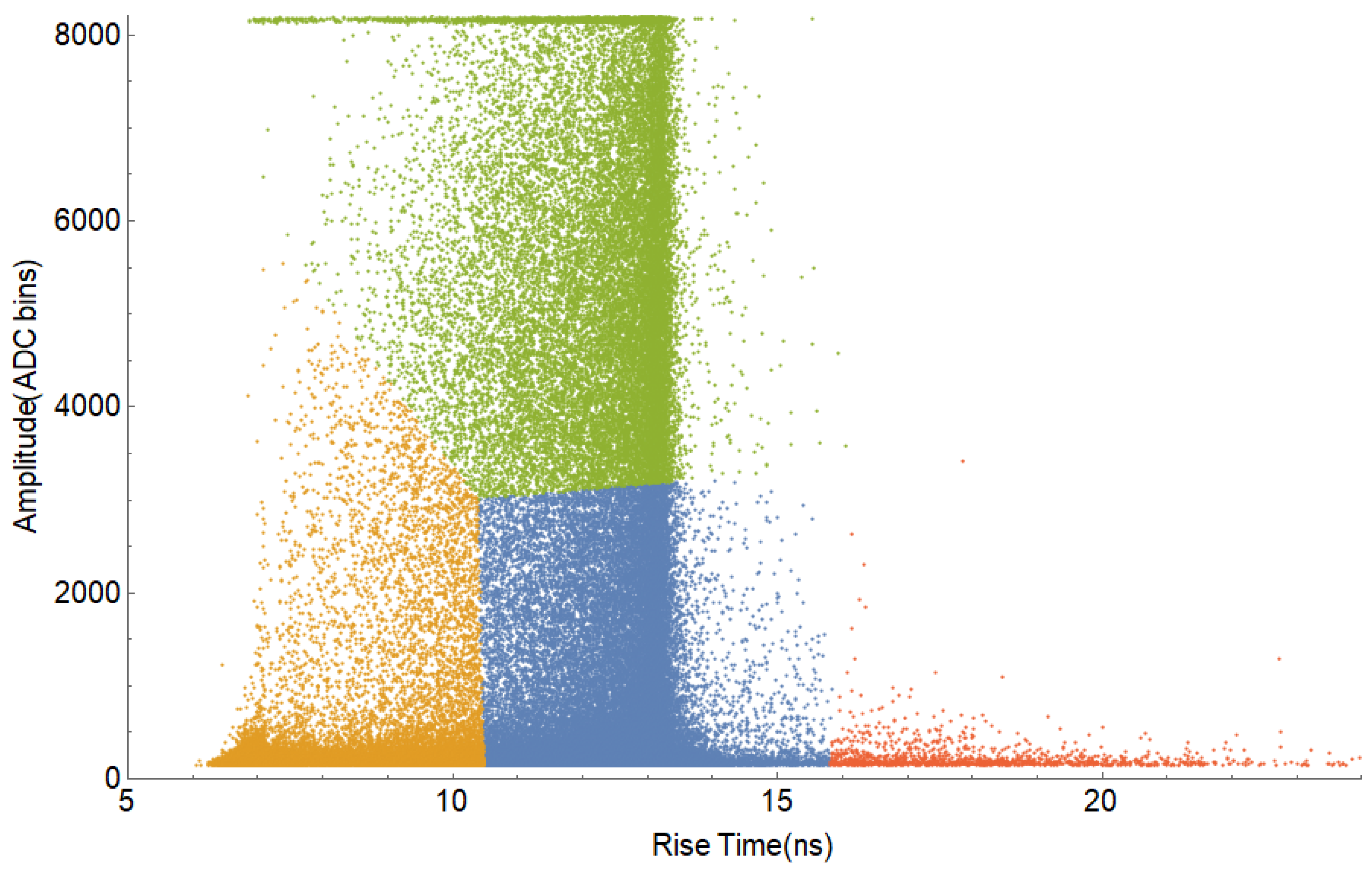
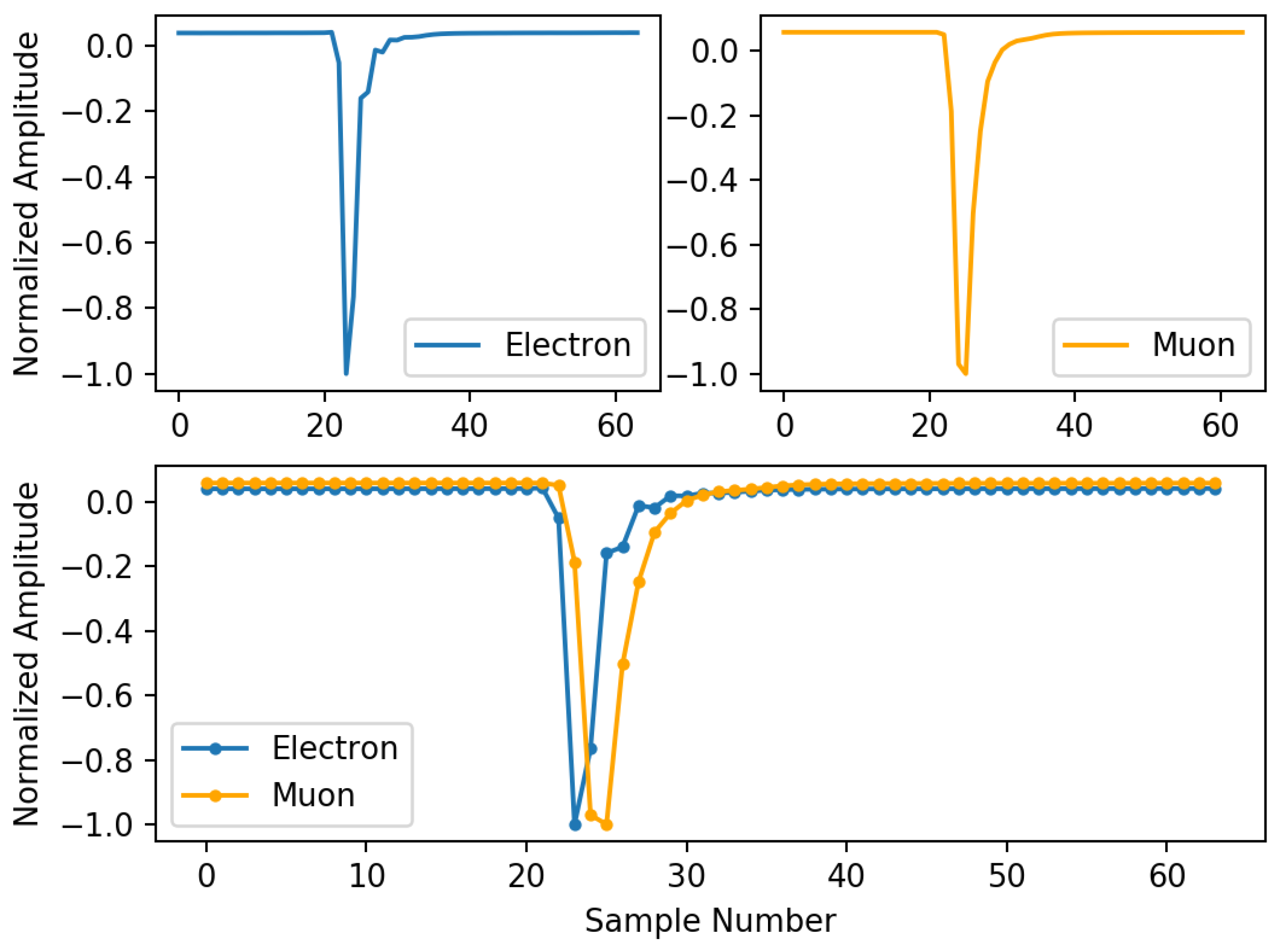
3.2. Data Set Analysis and Pulse Discrimination Criteria

Several data sets were collected from a water Cherenkov detector (WCD) at the Escuela de Ciencias Físicas y Matemáticas in Universidad de San Carlos de Guatemala (ECFM-USAC). The signal was sampled at 125 MHz with 14-bit resolution using a Red Pitaya on-board ADC.

Some feature extraction was performed in the incoming signal to obtain the rise time (10% to 90% of the output step height) and the amplitude needed to discriminate among the different types of signals. In Figure 2, a typical distribution of the pulses captured by the DAQ is presented. To have an objective classification criteria, we run a k-means clustering algorithm of four partitions (Figure 3) to select the border parameters to differentiate the signals. To stay in the safe zone, in this experiment, only the central portions of the muon and of the electron clusters have been used to label the data selected for the supervised training.

The classification criteria selected for the pulse shape discrimination is the following:

• Electron: amplitude below 3000—Rise time: between 6 and 9 ns.
• Muon: amplitude from 3000 to 8000—Rise time: between 11 and 15 ns.
• Electrical Discharge: amplitude greater than 8000 or data that do not fall in the previous categories.

To validate our criteria, we study the physics of the muon decay phenomenon [56]. The muon mean lifetime is ~2.196 µs, and it was used to determine the reference pulses corresponding to a typical muon and electron. Because charge must be conserved, one of the products of muon decay is always an electron. This can be used in such a way that pairs of pulses whose time difference fits the model were searched to use as reference, as we can observe in Figure 4. This procedure has been used in other context to measure muon half-life [57].

Moreover, the muon has higher mass than the electron, (~200 times more). Having a much greater mass, the muon can travel further into the medium producing longer pulses. Because electrons have lower mass, they interact more in the medium, which makes them deposit their energy more quickly, producing shorter pulses. A similar discussion was also presented by Salazar [19].

Based on this information, the training data set was generated. The ground truth for each pulse is indicated by adding an extra column, with an identification value for each type of signal: 0 for electron, 1 for muon and 2 for electric discharge, as shown in Figure 5.

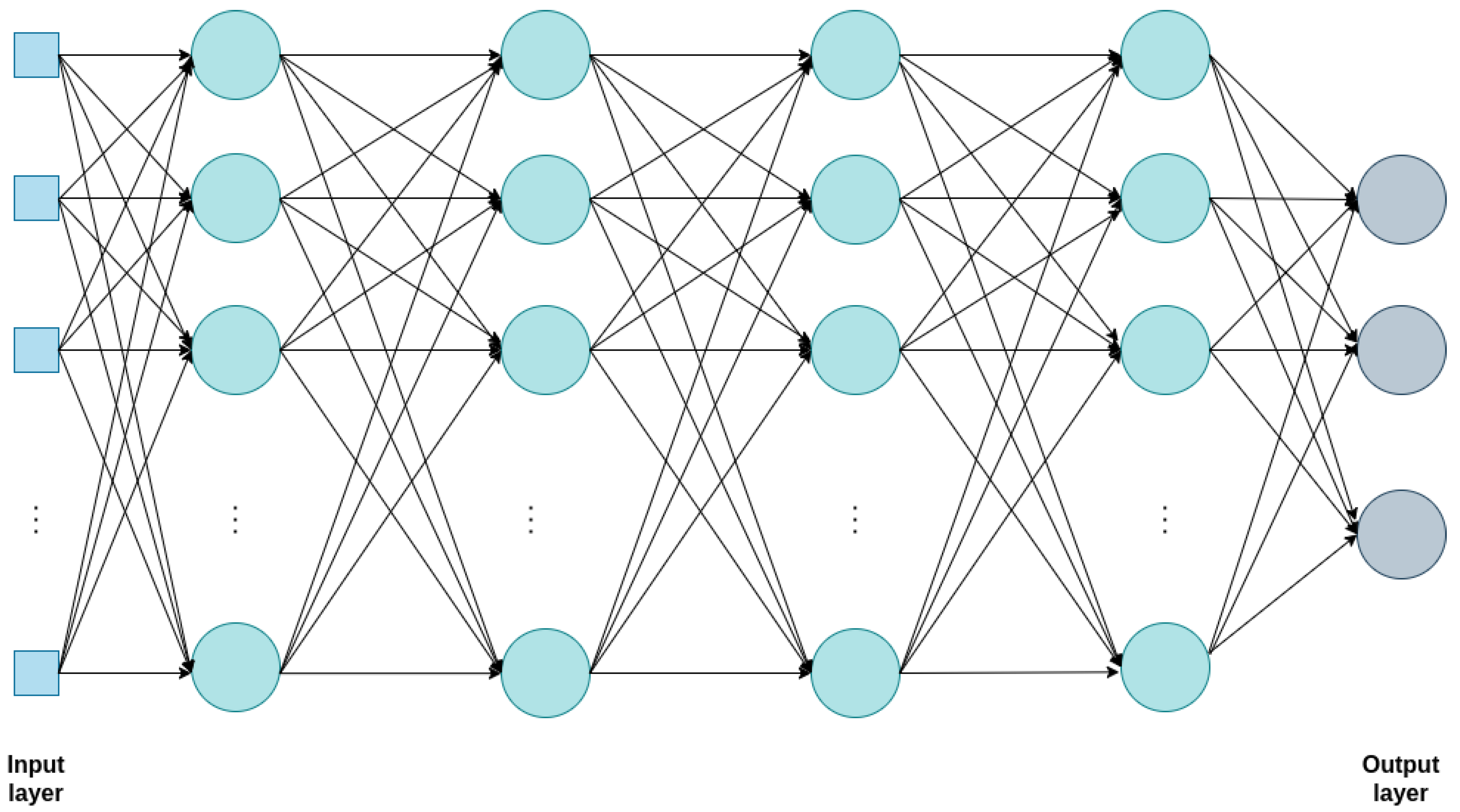
3.3. Neural Network Approach Based on Multilayer Perceptron

An artificial neural network (ANN) [58] is composed of neuron (or node) interconnections arranged in different layers, usually an input layer, middle or hidden layers and the output layer, where a prediction is generated. The connections between the neuron and the inputs ($x_i$) are called weights ($w_i$). Each node has several inputs and only one output, and the ANN uses a nonlinear activation function to compute the output value. This description can be observed in Figure 6 and is mathematically represented by Equation (1).

$$y=f((\sum _i{x}_i{w}_i)+b)$$

(1)

where $x_i$ are the inputs, $w_i$ are the weights, b represents the bias, f the activation function and y the final output of the neuron.

In an ANN-based classifier, an input is mapped into a specific class. For this task, an ANN goes through a supervised training step to recognize patterns: the network compares its actual output with the desired output. The difference between these two values is adjusted with backpropagation.

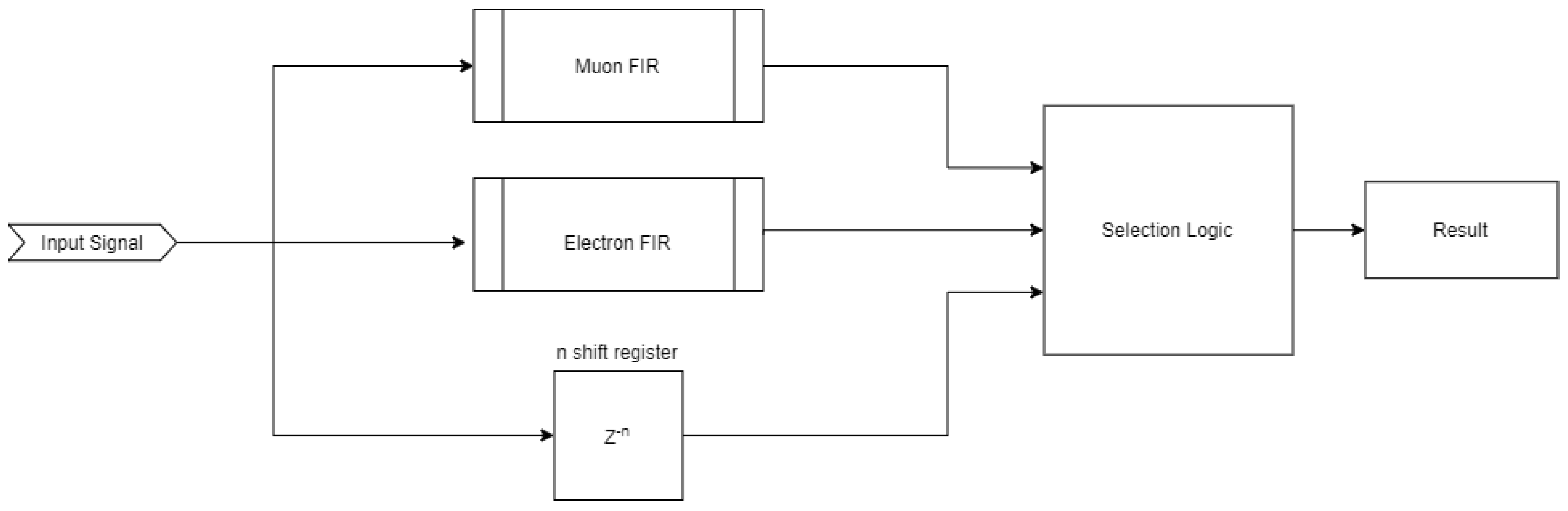
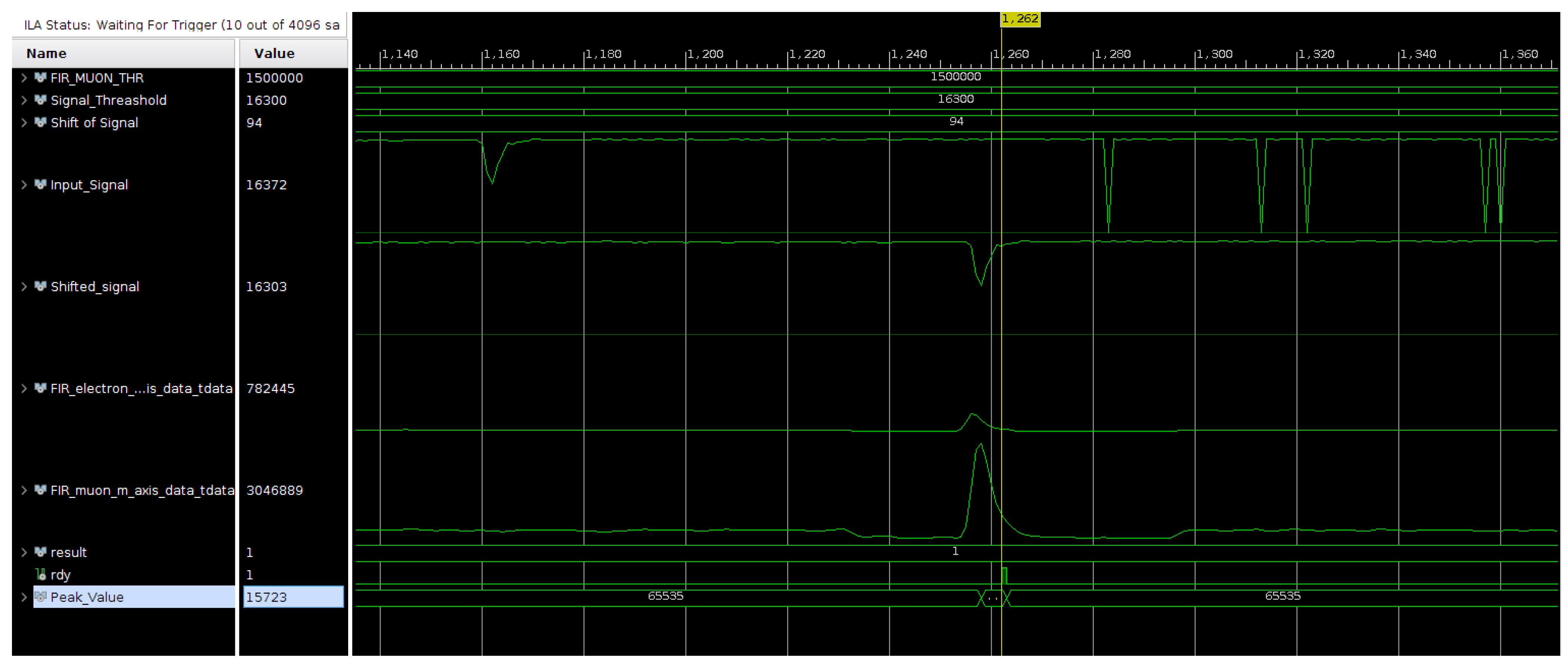
3.4. FIR Correlation Approach

The Pearson correlation function between a pair of N-element data vectors is stated in Equation (2), where x is the input signal and y the reference pulse. $\overline{x}$ and $\overline{y}$ are their respective average values and ${\sigma }_x$ and ${\sigma }_y$ are their corresponding standard deviations. The result $\rho (x,y)$ is closer to 1 when the likelihood between both signals is closer.

$$\rho (x,y)=\frac{{\displaystyle \sum _{i=0}^{N-1}}\left[(x_i-\overline{x})(y_i-\overline{y})\right]}{{\sigma }_x{\sigma }_y}=\frac{1}{{\sigma }_x}\sum _{i=0}^{N-1}\left[(x_i-\overline{x})\left(\frac{y_i-\overline{y}}{{\sigma }_y}\right)\right]$$

(2)

If the reference signal is static, $y_i$, $\overline{y}$ and ${\sigma }_y$ are constants. This expression $((y_i-\overline{y})/{\sigma }_y)$ is the standard score normalization, and it will be used to calculate the coefficients of the FIR ($c_i$). To avoid using floating-point coefficients, the result is multiplied by a scaling factor of n bits, as shown in Equation (3). To establish a good reference signal, a large number of previously classified pulses are normalized using the standard score and averaged for each point. For this experiment, each reference (electron and muon) was created using 42,000 pulses, and the coefficients have a scaling factor of n = 14.

$$c_i=\frac{y_i-\overline{y}}{{\sigma }_y}{2}^n$$

(3)

The signal will be processed in parallel by two FIR filters with its corresponding reference. Because ${\sigma }_x$ and $\overline{x}$ will be the same for both FIR inputs, the correlation for both filters will be scaled in the same proportion. The selection logic then can be simplified to take the output of both filters and make a decision based on the higher correlation through the duration of a pulse, establishing a rejection threshold. Taking this into consideration, the output equation of the filter is defined by Equation (4).

$${\rho }_{out}=\sum _{i=0}^{N-1}{x}_i{c}_i$$

(4)

As seen in Figure 2, the main criteria to differentiate between muons and electrons are the rise time and the amplitude of the pulses. The first criterion to classify the signals is the rise time of the pulse. This is difficult to achieve due to the DAQ sampling time of 8 ns, which is smaller than the rise time of the electron. To overcome this problem, we study the overall form of the pulse to perform the selection. A comparison between electron and muon reference pulse normalized in amplitude to 1 to highlight their differences is shown in Figure 7. At the current sampling rate, the peak of the electron is reached by only one data point. In contrast, a muon may have two or three data points before reaching the peak; these variations give the muon reference a “flattened” peak shape. A slower rise time has the effect of a smoother curve after the peak. The correlation between both references is 0.62; if we set a correlation value of 0.9 or higher to accept a pulse as a particle, the differences between the pulses is enough to use them as a criteria of classification.

The amplitude of the pulses is the second criteria used to make a decision. As is shown in Figure 3, electrons typically have lower amplitude compared with muons (orange cluster). However, some muons may have low amplitude as well (blue cluster). At higher amplitudes (green cluster), it is possible to find muons and electrical discharges produced by the PMT. Some electrical discharges may saturate the signal, as it is seen in top of the green section of the cluster, making it easy to separate them from a muon. For the purpose of analysis, we will call the value that separates the amplitude between muon and electrons the muon threshold (${\mu }_T$).

The selection logic decides that a pulse is starting by the crossing of a threshold by the signal. This will start a state machine that will search for the maximum amplitude of both the correlation results (${\rho }_{\mu }$ and ${\rho }_e$) and the amplitude of the peak ($P_x$). When the signal crosses back, the threshold the state machine will consider it as the end of a pulse and perform a selection according the collected information and the criteria established in the previous paragraphs. The selection criteria uses the following logic:

• If ${\rho }_{\mu }$ and ${\rho }_e$ are greater than a base reference value ($R\approx 0$) pass to the next criteria. This will discard uncorrelated signals like electrical discharges.
• If ${\rho }_e>{\rho }_{\mu }$, the signal is an electron, else if ${\rho }_{\mu }>{\rho }_e$, the signal is a muon.
• In the case of ${\rho }_e={\rho }_{\mu }$, the amplitude of the peak $P_x$ will be used to take the decision. If $P_x\ge {\mu }_T$, the result is a muon.
• If the signal is in saturation $(P_x=max\left(x\right))$, the selection logic will classify it as an electrical discharge.

4. Implementation

In this section, we present the implementation of the two approaches for pulse shape discrimination and the results obtained for each case, including accuracy for the classification, FPGA resource utilization and latency.

To describe the neural network architecture, we selected TensorFLow, Keras and QKeras. The package hls4ml was used to map the neural network inference to the Vivado High-Level Synthesis tool.

We selected XC7Z020 and ZU9EG as target boards, with a clock of 5 ns, using Xilinx Vivado Design Suite 2019.1.

4.1. Neural Network Implementation

The multiclass classification problem is based on distinguishing three types of pulses: muon, electron and electric discharges from the raw signals. The neural network was designed and implemented using the open-source software library Keras [59] with TensorFlow [60] as back end. The architecture is based on dense layers with four hidden layers and can be seen in Figure 8.

Regarding the activation functions, for each layer, a rectifier linear unit (ReLU) was employed, and to perform the calculation of the final probability for each class, Softmax was used in the output layer.

During the training, we implemented k-fold cross-validation, which leads us to use $k-1$ folds as training data, with $k=10$. The training parameters were configured as follows: batch size: 512, epochs: 32, optimizer: Adam [61] with a learning rate equal to 0.0001. To obtain the final model, three training stages were performed, keeping the base parameters:

• Training 1: for the base network to verify the performance with L1 regularization for kernels and bias in each layer with a value of 0.0001.
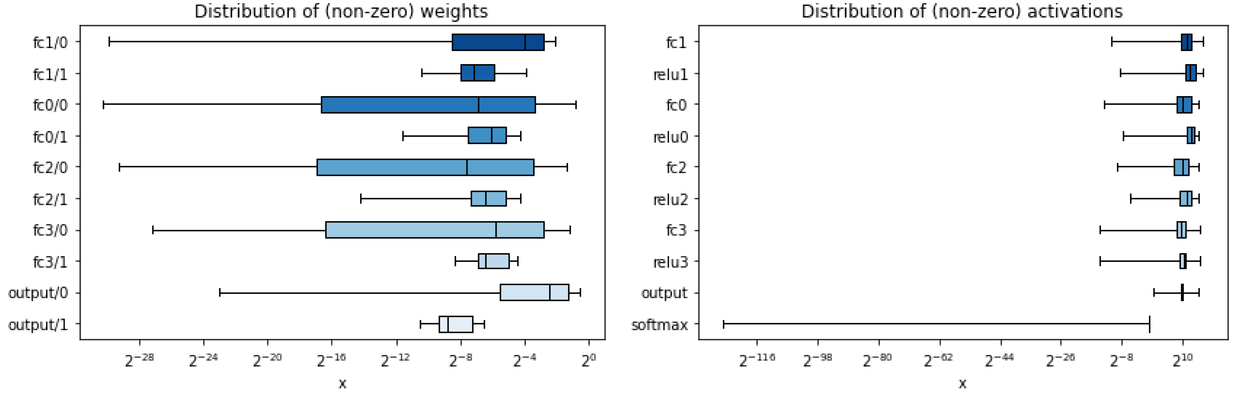
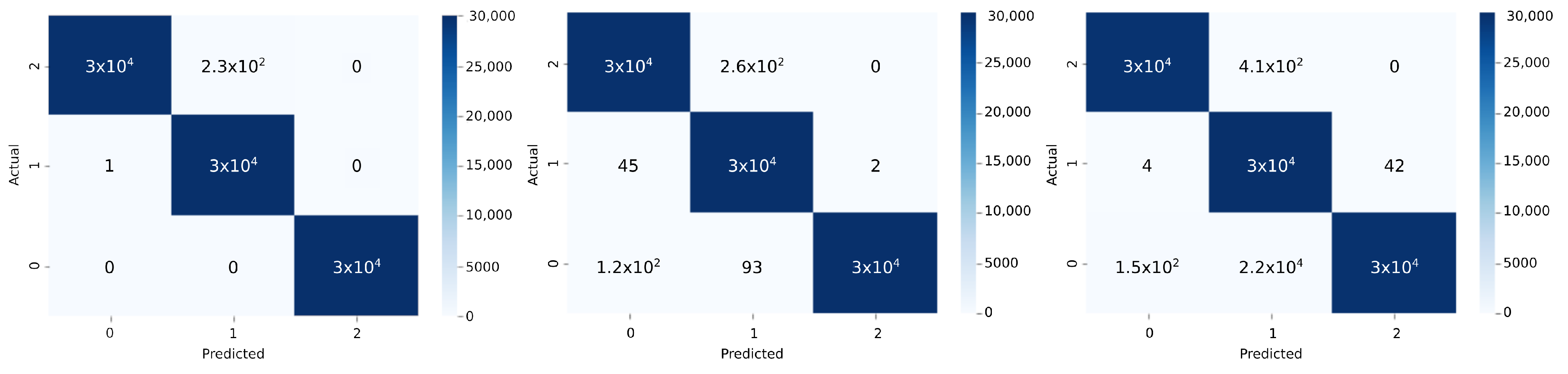
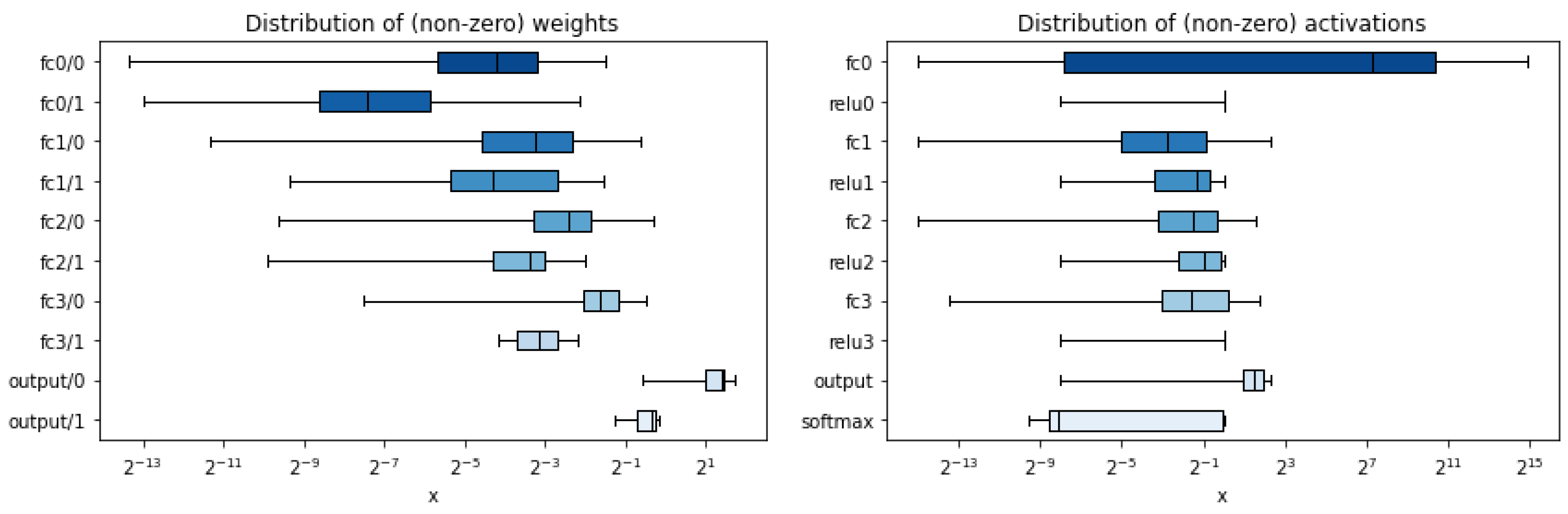
• Training 2: for the quantized network with L2 regularization for kernels and bias in each layer with a value of 0.0001 was used. In this implementation, a better accuracy was obtained compared with L1 normalization when training the quantized network. The quantization was performed with 16 bits in the input and first dense layer, 9 bits for weights and bias for the rest of the layers and 18 bits for the last layer with Softmax activation function.
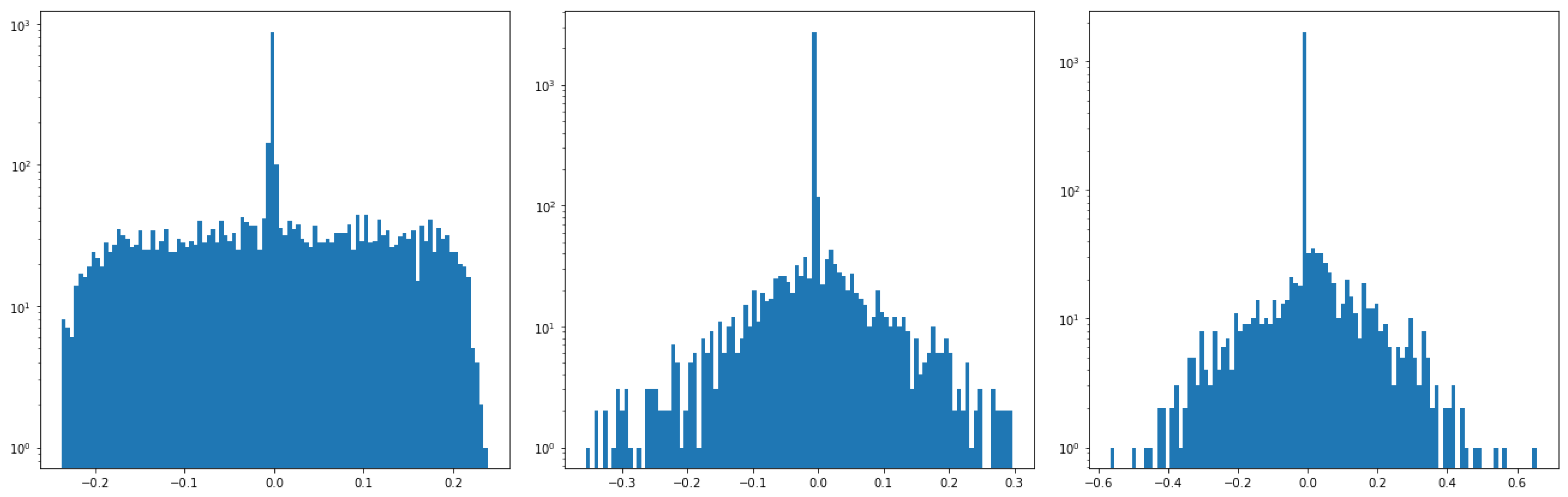
• Training 3: for pruning the network.

As the final goal is the implementation of PSD in the FPGA/SoC platform, model compression was performed through quantization and pruning, reducing redundant parameters. Benefits of compression and an analysis of the state of the art can be found in [62]. For this task, the network was described and trained using QKeras [63], a framework that is complementary to Keras for quantization, where each layer of the base model can be replaced by their counterparts (QDense, QConv1D, QConv2D, QActivation, etc.). The work [64] presented the integration between QKeras and hls4ml, showing how this technique helps to reduce resource consumption while retaining high accuracy when implemented on FPGA accelerators. The work in [65] used hls4ml to compress deep neural network models to binary and ternary precision, showing the positive impact in FPGAs.

The bit precision for weights and bias to train using QKeras was selected based on the profiling provided by hls4ml. Once the base model was obtained using TensorFlow+Keras, it was compiled using the package to analyze the weights and bias precision. The profiling obtained is presented in Figure 9.

The final accuracy reported for the quantized network after training was lower than the original one. After the quantization process, the second step to reduce resource consumption and inference times was to compress the model using pruning. For this, TensorFlow Model Optimization toolkit was used, with a target sparsity value of 0.7, keeping the sparsity constant during training.

After the compression stage, the model was saved and exported to .h5 file to map the neural network inference into the FPGA. For this step, we chose to use the hls4ml package, which is designed specifically for applications in the context of high-energy physics, assuring low latency for inference and integrating the translation flow with Vivado HLS, which supports C, C++ and System C code to generate the final RTL. The use of directives provided by the tool facilitates code optimization through parallel techniques like loop pipeline, loop unrolling, array partition and array reshape, among others. The designer can specify for each solution different combinations of directives and, through the comparison reports provided by Vivado HLS, decide which is the best option based on hardware resources and latency criteria.

Once the HLS project is created with hls4ml, it is ready for synthesis of the IP core with directives already applied in the final firmware, mainly using PIPELINE, UNROLL and ARRAY PARTITION pragmas. In the absence of specified parameters for each layer and the overall project, the tool will keep the default configuration, including the FPGA part, reuse factor, data type and optimization for latency or resource, among others. For this application, for the complete project, the reuse factor for all the layers was set as 1 and the strategy for optimization was to improve latency.

For this implementation, hls4ml adopted the data types generated by the training step using QKeras. Inside HLS, this will be reflected by the use of ap_fixed<W,I,Q,O,N> data type, where W is the word length in bits, Q is the quantization mode, O is the overflow mode and N is the number of saturation bits. For this part, the final precision with fine granularity was configured as follows:

• ap_fixed<17,1> for weights and bias for the first fully connected layer;
• ap_fixed<9,1> for weights and bias for the rest fully connected layers;
• ap_fixed<9,1,AP_RND,AP_SAT> for all activation layers based on the ReLU;
• ap_fixed<19,9> for weights and ap_fixed<9,1> for bias corresponding to the output layer;
• ap_fixed<23,15> for the model.

From the experiments, HLS reports showed that Softmax activation function in the last layer increased the clock cycles. For this reason and in this application, a decision scheme based on the output of the last fully connected layer was implemented, considering a threshold for each class to perform the classification, obtaining less accuracy than the pruned version but with less latency, which is crucial for online implementation.

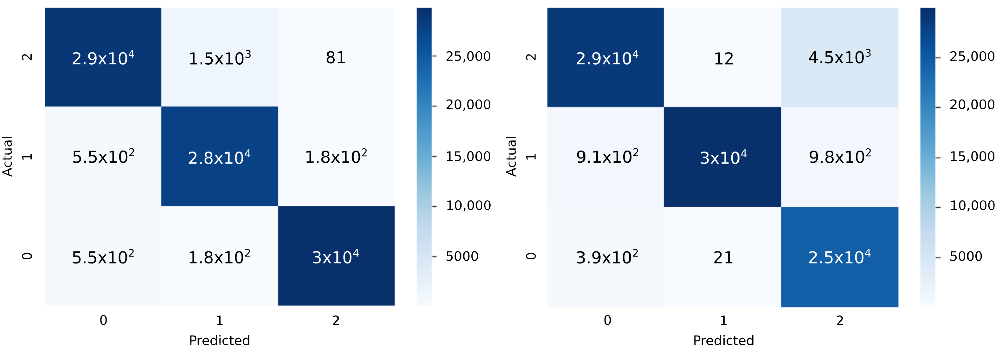
Neural Network Results

In this section, we present the results obtained with the neural network implementation for pulse shape discrimination in the context of WCD. For the different training steps, the data set was composed by 500,000 signals for each type of pulse and with k-fold cross-validation, and 20% of the train data set was used for validation. For testing, we used an extra set of data composed by 30,000 signals for each class.

Table 1. Accuracy obtained for the different approaches.

Implementation	Accuracy
Base network	99.67%
Quantized network with L1 norm	99.02%
Quantized network with L2 norm	99.24%
Pruned network	98.83%

presents the accuracy obtained for each neural network implementation, and as we can observe, the accuracy was reduced during the compression stage.

The resulting confusion matrices for all the previous steps can be seen in Figure 10, showing network performance for the classification task, where label 0 represents the electron, label 1 corresponds to the muon and label 2 is related to electric discharge. To generate them, the inference task was performed with a test composed by approximately 30,000 signals for each class.

As an example to observe the impact of compression, the histograms of weights corresponding to the first layer for the designed networks before and after quantization and pruning are presented in Figure 11. It can be noticed how the weights were affected in the different steps of the design, which will have a direct impact in the resource utilization of the hardware. A weight profiling is presented in Figure 12 after model compression.

With the final model generated, the inference was performed to verify its functionality, reporting an execution time of 0.0446 s for a single signal in an CPU with AMD Ryzen 5, 8 GB RAM, Radeon Vega 8 Graphics, Ubuntu 18.04.5 LTS.

Regarding HLS implementation for the IP core, we perform a comparison for different solutions mainly based on applied directives, reuse factor and the final activation function. Hardware resources and latency estimations reported by Vivado HLS can be seen in

Table 2. HLS reports comparison. Solutions 1 and 5 without directives. Solutions 2 and 6 with directives applied by hls4ml and Softmax as activation function. Solutions 3 and 7 with directives applied by hls4ml, PIPELINE to improve the interval, without Softmax and with a reuse factor of 1 for all the layers. Solutions 4 and 8 with directives applied by hls4ml, PIPELINE to improve the interval, without Softmax and with a reuse factor of 8 for all the dense layers.

Solution	Directives	Estimated Clock [ns]	Clock Cycles	Inference Clock Cycles	Interval	BRAM	DSP	FF	LUT
ZU9EG
1	No	4.653	36,917	36,848	36,917	23	2	2407	5732
2	Yes + Softmax	4.653	18,526	18,457	18,526	2	1245	26,192	180,066
3	Yes + NS + RF: 1	4.251	84	19	64	0	1235	27221	167,158
4	Yes + NS + RF: 8	4.993	115	50	64	0	155	38,571	141,443
XC7Z020
5	No	6.508	91,777	91,707	91,777	23	2	4313	6952
6	Yes + Softmax	6.508	40,063	39,993	40,063	2	1245	188,626	171,599
7	Yes + NS + RF: 1	4.350	121	55	64	0	1235	189,059	159,351
8	Yes + NS + RF: 8	5.561	143	77	64	0	155	76,286	118,936

, with axis interface for input/output and s_axilite interface for control signals and a clock of 5 ns.

For the XC7Z020 family, without directives, all the resources were used less than 100%, but with a high amount of clock cycles reported as we can observe with Solution 5. On the other side, fewer clock cycles for the inference can be obtained, but the resource utilization of the board exceeds its capability, as presented with Solutions 7 and 8. In this situation, the option reuse factor from hls4ml could help to obtain a good compromise between latency and hardware utilization, as we can observe with Solutions 4 and 8, where a reuse factor of 8 was configured. Regarding the ZU9EG family, for all the tests carried out, the FPGA resources were used less than 100%, observing that the best implementation was Solution 3, with an overall latency of 84 cycles, of which 19 clock cycles correspond to the neural network inference.

Due to the data dependency on the operations that are performed by the inference, the optimal implementation was obtained when the directive ARRAY_PARTITION is configured with total partition for the data structures, increasing the utilization of hardware resources. A PIPELINE directive for Solution 4 and Solution 8 is at top-level function, allowing data streaming processing with a final throughput equal to 64 clock cycles.

From the previous analysis, and taking into account an online muon–electron discrimination, Solution 3 was selected to be exported as IP core and implemented using Vivado Design Suite to obtain the final resource utilization, latency and power consumption estimation.

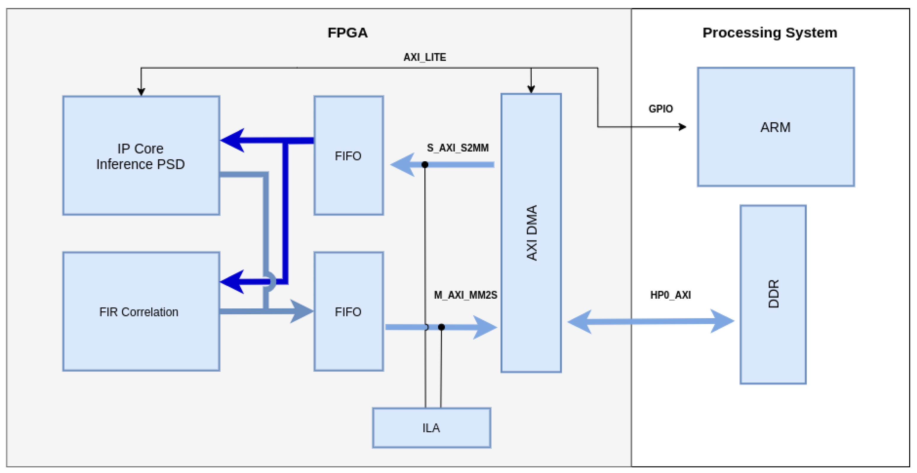
4.2. FIR Implementation

A block diagram of the muon–electron correlation discriminator is shown in Figure 13. The FIR filter is used to do the correlation of the input signal with an output result given by Equation (2). The coefficients are calculated by standard score normalization and averaging typical signals like the ones in Figure 5 using Equation (3).

A RAM-based shift register block provides the latency to the signal to align it with the the outputs of the filters to be used as inputs in a selection logic block. The selection logic state machine starts when the signal crosses a threshold. It is implemented as a peak holder until the signal crosses down the threshold again. The selection logic is done in parallel until this moment. After the signal crosses down the threshold, the result will be available in the next clock cycle, indicated by a “ready” signal. After the ready signal, the system is ready to receive another pulse. The possible outcomes are 0 to electron, 1 to muon, 2 to electrical discharge and 3 for other type of signal. The input signals and the selection logic of one real pulse, captured using Vivado’s Integrated Logic Analyzer (ILA), are shown in Figure 14. For this example, the acquisition starts when the shifted signal crosses the threshold. The yellow line shows the moment when the output signal is presented. In this case, the output of the muon FIR is higher than the electron, leading to the decision that the pulse is a muon. The output also returns the peak of the signal.

In this image, the latency of the input signal and the output of the FIR filters are also visible. The overall latency measured with the ILA is 94 clock cycles and used as a parameter of the shift register. This configuration has a dead time of 1 clock cycle before it is ready to measure the next pulse. The reported utilization for the following approach is detailed in

Table 3. Resource utilization of the FIR-based correlation pulse discrimination.

	ZU9EG	XC7Z020	ZU9EG	XC7Z020	ZU9EG	XC7Z020	ZU9EG	XC7Z020
Description	BRAM		DSP		FF		LUT
Shift Register	0	0	0	0	576	688	1088	1088
FIR electron	0	0	64	64	2538	2838	58	188
FIR muon	0	0	64	64	2514	2818	58	188
Selection Logic	0	0	0	0	146	5778	378	12,508
Total	0	0	128	128	5767	12,122	1582	13,972

.

5. Analysis of Results

To evaluate the performance of both methods, a known data set is transmitted to the FPGA by DMA transfer using the embedded microprocessor in the SoC. The data is stored in a FIFO and the reading is enabled by the processor after the storage is done to simulate a readout from an ADC. The result of the classification performed in the FPGA is stored in another FIFO and sent back to the processor, which validates the results. The chain of transmission and all of the elements of the test design are illustrated in Figure 15.

The data set is composed of 90,000 events previously classified and equally distributed in electrons, muons and electrical discharges. The integrity of the data is verified using the ILA. The confusion matrices corresponding to the results for both methods are shown in Figure 16.

We can observe that the neural network is able to maintain consistent performance for each type of signal, while the accuracy obtained is less compared to the results shown in Table 1, with 96.31% for electron, 92.88% for muon and 99.14% for electric discharges. This behavior is mainly due to the quantization chosen with hls4ml and the replacement of the Softmax function in the output layer.

A further comparison between the matrices is shown in

Table 4. Sensitivity, specificity, positive and negative predicted value comparison between the neural network and FIR.

	Sensitivity (TPR)		Specificity (TNR)		PPV		NPV
	NN	FIR	NN	FIR	NN	FIR	NN	FIR
Electron	94.83%	86.54%	98.15%	97.73%	96.35%	95.71%	97.36%	92.54%
Muon	97.46%	94.07%	97.26%	99.94%	94.34%	99.89%	98.79%	96.89%
Electric Discharges	97.62%	98.38%	99.56%	91.62%	99.14%	82.02%	98.78%	99.32%
Overall Accuracy	96.62%	92.50%
Kappa Coef.	0.949	0.887

. For both matrices, the true positive and negative rates (TPR and TNR), also called sensitivity and specificity of the matrix, were calculated to measure the percentage of pulses correctly identified. The positive and negative predicted values (PPV and NPV) were calculated to compare the amount of true positive and negative pulses. While it is true that both have good results, the neural network is consistently better at characterizing electrons. In the case of muons and electrical discharges, the neural network has mixed results. The FIR has significantly higher precision in detecting muons with less sensitivity. The FIR system sensitivity to electrical discharges and significantly low precision is expected due to the trigger condition in the state machine. This allows detection of a much larger number of electrical discharges by not depending on a large acquisition window to analyze it. However, some electrical discharges may produce some free electrons in the PMT that may produce small currents that may be confused with electrons. This is evident in Figure 16, where the number may be determined by observing the relation of electrical discharges and electrons. Finally, the neural network presented higher overall accuracy and Kappa coefficient than the FIR correlation system.

It is worth mentioning that in both cases, the number of samples per pulse may be marginal to conduct the analysis.

A higher sampling rate may ease the discrimination by showing further differences among the different types of signals.

A comparison of the execution time that each method used for discrimination is presented in

Table 5. Execution time comparison among artificial neural networks (ANNs) using CPU, FPGA and the FIR correlation method.

Method	Execution Time [s]
ANN-CPU	44,000
ANN-FPGA	0.848
FIR-FPGA	0.752

. As reference, the execution time of an ANN running on a CPU with AMD Ryzen 5, 8 GB RAM, Radeon Vega 8 Graphics, Ubuntu 18.04.5 LTS, using Jupyter Notebook and Python is included in the comparison. The FPGA is running with a 125 MHz clock, in correspondence with the sampling rate of the signal.

As can be seen, both methods implemented on the FPGA have big differences in magnitude order compared with the CPU. Between them, there is a difference of 96 ns, corresponding to 12 clock cycles.

The main advantage of the ANN inference-based design for PSD is obtaining a small latency for the signal classification using FPGA. Although the overall accuracy with this approach is less than that found in the literature, this behavior was expected after the model compression process due to the elimination of redundant parameters and bit reduction.

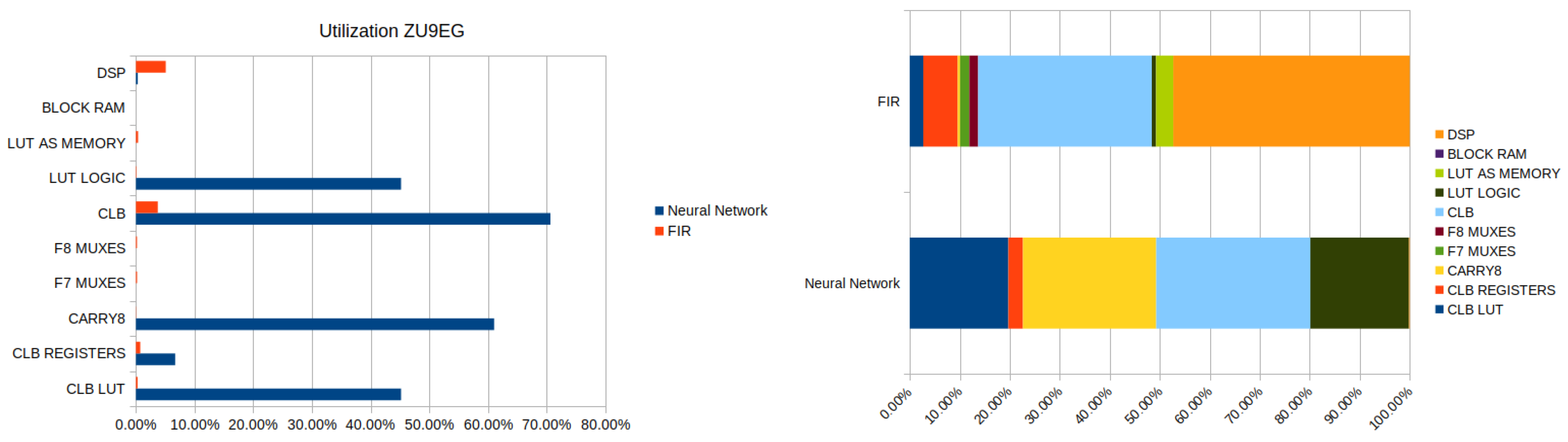
Resources Utilization and Power Consumption

As mentioned in previous sections, both approaches were implemented on a ZU9EG and XC7Z020 chip. Specific resources utilization are shown in its respective sections. For comparison, the following analysis are performed in a ZU9EG Zynq UltraScale+ chip. The information was collected using the postimplementation reports provided by Vivado. In Figure 17, a comparison between the resources occupancy (left) and the type of resources that both methods utilize (right) is shown.

As it can be seen, the FIR approach uses much fewer resources than the neural network approach; however, in the right graphic, it is visible that the major resource used by the FIR is the DPS blocks followed by a similar percentage of configurable logic blocks (CLBs). In contrast, the neural network uses a higher number of CLBs and block RAM units to perform the analysis. This may be further optimized in the HLS design.

The increased number of components used by the neural network is reflected in the power consumption of the design. The estimated power consumption between both methods is shown in Figure 18.

It is worth noticing that the FIR-based approach is heavily dependent on the threshold parameters. This may lead to additional logic blocks in the case of the need of dynamical adjustment of the parameters. The occupation may vary depending on the complexity of these additional blocks.

6. Conclusions and Future Work

In this research, we implemented on FPGA two methods for pulse shape discrimination between muon and electron pulses for a water Cherenkov detector (WCD)—one based on finite-impulse-response (FIR)-based correlation, and the other on an artificial neural network (ANN). The data set used for the experiment was captured from a WCD to use real pulses for the analysis.

Regarding the neural network, we used the novel hls4ml package to build the ANN inference model into the FPGA, assuring low latency. The whole design process is described, from the neural network topology up to the final model, including training and compression techniques such as quantization and pruning.

An FIR-based correlation was implemented with its selection logic for particle classification. The coefficients were calculated using a standard score normalization. The correlation calculation was done in parallel and the decision was made in a single clock cycle after the pulse ended.

A Xilinx ZU9EG UltraScale+ SoC running on a ZCU102 development board was used for the experiment running with a clock frequency of 125 MHz. The results showed an overall accuracy on particle discrimination of 96.62% for the ANN and 92.50% for the FIR-based correlation, with execution times of 848 ns and 752 ns, respectively.

The resources and power consumption comparison between both methods shows that the ANN, while having higher overall accuracy, presented higher resources utilization on the FPGA. In contrast, the FIR filter has significantly less accuracy but also less resources utilization. This is directly related to the power consumption. The execution times for both methods are on the same order of magnitude, and their differences are negligible compared with the execution time on a CPU.

Both methods can be implemented along with an FPGA front-end acquisition system for online analysis to save computational resources in postprocessing.

As this is a study based on the shape of the pulse, it can be inferred that, for both methods, a higher sample rate should improve the results due to the increase of information available to perform the discrimination. A future study is planned using a 500 MHz sampling rate for the data acquisition.

Future developments will include improving the quantization strategy, a comparison with other neural network topologies to analyze the impact in accuracy and hardware implementations. Stream processing will also be added to the neural network approach.

The overall accuracy of the FIR system may still be improved by adding a dead time after an electrical discharge to reject possible artifacts that may be confused with electrons; however, the duration of this time needs to be further studied.

References

1. Pierre Auger Collaboration. The Pierre Auger Cosmic Ray Observatory. Nucl. Instrum. Methods Phys. Res. Sect. A Accel. Spectrometers Detect. Assoc. Equip. 2015, 798, 172–213. [Google Scholar] [CrossRef]
2. DeYoung, T. The HAWC observatory. Nucl. Instrum. Methods Phys. Res. Sect. A Accel. Spectrometers Detect. Assoc. Equip. 2012, 692, 72–76. [Google Scholar] [CrossRef]
3. Castellina, A. AugerPrime: The Pierre Auger Observatory Upgrade. EPJ Web Conf. 2019, 210, 06002. [Google Scholar] [CrossRef]
4. Allard, D.; Allekotte, I.; Alvarez, C.; Asorey, H.; Barros, H.; Bertou, X.; Burgoa, O.; Berisso, M.G.; Martínez, O.; Loza, P.M.; et al. Use of water-Cherenkov detectors to detect gamma ray bursts at the Large Aperture GRB Observatory (LAGO). Nucl. Instrum. Methods Phys. Res. Sect. A Accel. Spectrometers Detect. Assoc. Equip. 2008, 595, 70–72. [Google Scholar] [CrossRef] [Green Version]
5. STEMLab. Red Pitaya 0.97 Documentation-Red Pitaya Developers Guide. 2017. Available online: https://redpitaya.readthedocs.io/en/latest/ (accessed on 30 December 2020).
6. Arnaldi, L.H.; Cazar, D.; Audelo, M.; Sidelnik, I. Preliminary results of the design and development of the data acquisition and processing system for the LAGO Collaboration. PoS 2019, ICRC2019, 175. [Google Scholar] [CrossRef]
7. Garcia Ordóñez, L.G.; Morales Argueta, I.R.; Crespo, M.L.; Carrato, S.; Cicuttin, A.; Perez, H.; Barrientos, D.; Levorato, S.; Valinoti, B.; Florian, W.; et al. DAQ platform based on SoC-FPGA for high resolution time stamping in cosmic ray detection. PoS 2019, ICRC2019, 266. [Google Scholar] [CrossRef]
8. De Rújula, A. An introduction to Cosmic Rays and Gamma-Ray Bursts, and to their simple understanding. arXiv 2007, arXiv:0711.0970. [Google Scholar]
9. Aab, A.; Abreu, P.; Aglietta, M.; Al Samarai, I.; Albuquerque, I.; Allekotte, I.; Almela, A.; Castillo, J.A.; Alvarez-Muñiz, J.; Anastasi, G.A.; et al. Observation of a large-scale anisotropy in the arrival directions of cosmic rays above 8 × 10¹⁸ eV. Science 2017, 357, 1266–1270. [Google Scholar]
10. Anchordoqui, L.A. Ultra-high-energy cosmic rays. Phys. Rep. 2019, 801, 1–93. [Google Scholar] [CrossRef] [Green Version]
11. Piron, F. Gamma-ray bursts at high and very high energies. Comptes Rendus Phys. 2016, 17, 617–631. [Google Scholar] [CrossRef]
12. Liu, G.; Aspinall, M.; Ma, X.; Joyce, M. An investigation of the digital discrimination of neutrons and γ rays with organic scintillation detectors using an artificial neural network. Nucl. Instrum. Methods Phys. Res. Sect. A Accel. Spectrometers Detect. Assoc. Equip. 2009, 607, 620–628. [Google Scholar] [CrossRef]
13. Chandhran, P.; Holbert, K.E.; Johnson, E.B.; Whitney, C.; Vogel, S.M. Neutron and gamma ray discrimination for CLYC using normalized cross correlation analysis. In Proceedings of the 2014 IEEE Nuclear Science Symposium and Medical Imaging Conference (NSS/MIC), Seattle, WA, USA, 8–15 November 2014; pp. 1–8. [Google Scholar] [CrossRef]
14. Fu, C.; Fulvio, A.D.; Clarke, S.; Wentzloff, D.; Pozzi, S.; Kim, H. Artificial neural network algorithms for pulse shape discrimination and recovery of piled-up pulses in organic scintillators. Ann. Nucl. Energy 2018, 120, 410–421. [Google Scholar] [CrossRef]
15. D’Mellow, B.; Aspinall, M.; Mackin, R.; Joyce, M.; Peyton, A. Digital discrimination of neutrons and γ-rays in liquid scintillators using pulse gradient analysis. Nucl. Instrum. Methods Phys. Res. Sect. A Accel. Spectrometers Detect. Assoc. Equip. 2007, 578, 191–197. [Google Scholar] [CrossRef]
16. Ammerlaan, C.; Rumphorst, R.; Koerts, L. Particle identification by pulse shape discrimination in the p-i-n type semiconductor detector. Nucl. Instrum. Methods 1963, 22, 189–200. [Google Scholar] [CrossRef]
17. Winyard, R.; Lutkin, J.; McBeth, G. Pulse shape discrimination in inorganic and organic scintillators. I. Nucl. Instrum. Methods 1971, 95, 141–153. [Google Scholar] [CrossRef]
18. Bartle, C. A study of (n,p) and (n,α) reactions in NaI(Tl) using a pulse-shape-discrimination method. Nucl. Instrum. Methods 1975, 124, 547–550. [Google Scholar] [CrossRef]
19. Salazar, H.; Villasenor, L. Separation of cosmic-ray components in a single water Cherenkov detector. Nucl. Instrum. Methods Phys. Res. Sect. A Accel. Spectrometers Detect. Assoc. Equip. 2005, 553, 295–298. [Google Scholar] [CrossRef]
20. Salazar, H.; Villasenor, L. Ground detectors for the study of cosmic ray showers. J. Phys. Conf. Ser. 2008, 116, 012008. [Google Scholar] [CrossRef]
21. Schoorlemmer, H.; Hinton, J.; López-Coto, R. Characteristics of extensive air showers around the energy threshold for ground-particle-based γ-ray observatories. Eur. Phys. J. C 2019, 79, 427. [Google Scholar] [CrossRef]
22. Zhu, J.; Gong, G.; Xue, T.; Cao, Z.; Wei, L.; Li, J. Preliminary Design of Integrated Digitizer Base for Photomultiplier Tube. IEEE Trans. Nucl. Sci. 2019, 66, 1130–1137. [Google Scholar] [CrossRef]
23. Mace, E.; Ward, J.; Aalseth, C. Use of neural networks to analyze pulse shape data in low-background detectors. J. Radioanal. Nucl. Chem. 2018, 318, 117–124. [Google Scholar] [CrossRef]
24. Griffiths, J.; Kleinegesse, S.; Saunders, D.; Taylor, R.; Vacheret, A. Pulse Shape Discrimination and Exploration of Scintillation Signals Using Convolutional Neural Networks. Mach. Learn. Sci. Technol. 2020, 1, 045022. [Google Scholar] [CrossRef]
25. Holl, P.; Hauertmann, L.; Majorovits, B.; Schulz, O.; Schuster, M.; Zsigmond, A.J. Deep learning based pulse shape discrimination for germanium detectors. Eur. Phys. J. C 2019, 79. [Google Scholar] [CrossRef]
26. Droz, D.; Tykhonov, A.; Wu, X. Neural Networks for Electron Identification with DAMPE. In Proceedings of the 36th International Cosmic Ray Conference—PoS(ICRC2019), Madison, WI, USA, 24 July–1 August 2019; Volume 358, p. 064. [Google Scholar] [CrossRef]
27. Villasenor, L.; Jeronimo, Y.; Salazar, H. Use of Neural Networks to Measure the Muon Contents of EAS Signals in a Water Cherenkov Detector. In Proceedings of the International Cosmic Ray Conference, Tsukuba, Japan, 31 July–7 August 2003. [Google Scholar]
28. Kohonen, T. Self-Organization and Associative Memory, 3rd ed.; Springer: Berlin/Heidelberg, Germany, 1989. [Google Scholar]
29. Guo, K.; Zeng, S.; Yu, J.; Wang, Y.; Yang, H. A Survey of FPGA-Based Neural Network Accelerator. arXiv 2018, arXiv:1712.08934. [Google Scholar]
30. Wei, X.; Liang, Y.; Cong, J. Overcoming Data Transfer Bottlenecks in FPGA-based DNN Accelerators via Layer Conscious Memory Management. In Proceedings of the 56th Annual Design Automation Conference 2019, DAC 2019, Las Vegas, NV, USA, 2–6 June 2019; p. 125. [Google Scholar]
31. Zhang, X.; Das, S.; Neopane, O.; Kreutz-Delgado, K. A Design Methodology for Efficient Implementation of Deconvolutional Neural Networks on an FPGA. arXiv 2017, arXiv:1705.02583. [Google Scholar]
32. Kim, J.H.; Grady, B.; Lian, R.; Brothers, J.; Anderson, J.H. FPGA-based CNN inference accelerator synthesized from multi-threaded C software. In Proceedings of the 2017 30th IEEE International System-on-Chip Conference (SOCC), Munich, Germany, 5–8 September 2017. [Google Scholar] [CrossRef] [Green Version]
33. Meloni, P.; Capotondi, A.; Deriu, G.; Brian, M.; Conti, F.; Rossi, D.; Raffo, L.; Benini, L. NEURAghe: Exploiting CPU-FPGA Synergies for Efficient and Flexible CNN Inference Acceleration on Zynq SoCs. ACM Trans. Reconfig. Technol. Syst. 2018, 11, 18:1–18:24. [Google Scholar] [CrossRef] [Green Version]
34. Duarte, J.; Han, S.; Harris, P.; Jindariani, S.; Kreinar, E.; Kreis, B.; Ngadiuba, J.; Pierini, M.; Rivera, R.; Tran, N.; et al. Fast inference of deep neural networks in FPGAs for particle physics. J. Instrum. 2018, 13, P07027. [Google Scholar] [CrossRef]
35. Nottbeck, N.; Schmitt, D.C.; Büscher, P.D.V. Implementation of high-performance, sub-microsecond deep neural networks on FPGAs for trigger applications. J. Instrum. 2019, 14, P09014. [Google Scholar] [CrossRef]
36. Xilinx. FIR Compiler v7.2. LogiCORE IP Product Guide PG149. Xilinx, 2020. Available online: https://www.xilinx.com/support/documentation/ip_documentation/fir_compiler/v7_1/pg149-fir-compiler.pdf (accessed on 30 December 2020).
37. Park, S.Y.; Meher, P.K. Efficient FPGA and ASIC Realizations of a DA-Based Reconfigurable FIR Digital Filter. IEEE Trans. Circuits Syst. II Express Briefs 2014, 61, 511–515. [Google Scholar] [CrossRef]
38. Malacari, M.; Farmer, J.; Fujii, T.; Albury, J.; Bellido, J.; Chytka, L.; Hamal, P.; Horvath, P.; Hrabovský, M.; Mandat, D.; et al. The first full-scale prototypes of the fluorescence detector array of single-pixel telescopes. Astropart. Phys. 2020, 119, 102430. [Google Scholar] [CrossRef] [Green Version]
39. Balmer, M.J.; Gamage, K.A.; Taylor, G.C. Comparative analysis of pulse shape discrimination methods in a 6Li loaded plastic scintillator. Nucl. Instrum. Methods Phys. Res. Sect. A Accel. Spectrometers Detect. Assoc. Equip. 2015, 788, 146–153. [Google Scholar] [CrossRef]
40. Szadkowski, Z.; Fraenkel, E.D.; van den Berg, A.M. FPGA/NIOS implementation of an adaptive FIR filter using linear prediction to reduce narrow band RFI for radio detection of cosmic rays. In Proceedings of the 2012 18th IEEE-NPSS Real Time Conference, Berkeley, CA, USA, 9–15 June 2012; pp. 1–8. [Google Scholar] [CrossRef]
41. Socha, P.; Miškovský, V.; Kubátová, H.; Novotný, M. Optimization of Pearson correlation coefficient calculation for DPA and comparison of different approaches. In Proceedings of the 2017 IEEE 20th International Symposium on Design and Diagnostics of Electronic Circuits Systems (DDECS), Dresden, Germany, 19–21 April 2017; pp. 184–189. [Google Scholar] [CrossRef]
42. Lusher, J.; Ji, J.; Orr, J. High-Performance Correlation and Mapping Engine for rapid generating brain connectivity networks from big fMRI data. J. Comput. Sci. 2018, 26, 157–164. [Google Scholar] [CrossRef] [Green Version]
43. Photonis. Photomultiplier Tubes Catalogue. 2007. Available online: https://hallcweb.jlab.org/DocDB/0008/000809/001/PhotonisCatalog.pdf (accessed on 30 December 2020).
44. Cotzomi, J.; Moreno, E.; Murrieta, T.; Palma, B.; Perez, E.; Salazar, H.; Villasenor, L. The water Cherenkov detector array for studies of cosmic rays at the University of Puebla. Nucl. Instrum. Methods Phys. Res. Sect. A Accel. Spectrometers Detect. Assoc. Equip. 2005, 553, 290–294. [Google Scholar] [CrossRef]
45. Abeysekara, A.; Aguilar, J.; Aguilar, S.; Alfaro, R.; Almaraz, E.; Álvarez, C.; Álvarez-Romero, J.d.D.; Álvarez, M.; Arceo, R.; Arteaga-Velázquez, J.; et al. On the sensitivity of the HAWC observatory to gamma-ray bursts. Astropart. Phys. 2012, 35, 641–650. [Google Scholar] [CrossRef] [Green Version]
46. Galindo, A.; Moreno, E.; Carrasco, E.; Torres, I.; Carramiñana, A.; Bonilla, M.; Salazar, H.; Conde, R.; Alvarez, W.; Alvarez, C.; et al. Calibration of a large water-Cherenkov detector at the Sierra Negra site of LAGO. Nucl. Instrum. Methods Phys. Res. Sect. A Accel. Spectrometers Detect. Assoc. Equip. 2017, 861, 28–37. [Google Scholar] [CrossRef]
47. XP Power. C Series, DC-HVDC Converter. 2020. Available online: https://www.xppower.com/portals/0/pdfs/SF_C_Series.pdf (accessed on 30 December 2020).
48. Texas Instruments. TLV5616C, TLV5616I 2.7-V to 5.5-V Low Power 12-bit Digital-to-Analog Converters with Power Down. 1997. Available online: https://www.ti.com/lit/ds/symlink/tlv5616.pdf?ts=1610973116569&ref_url=https%253A%252F%252Fwww.google.com%252F (accessed on 30 December 2020).
49. Genolini, B.; Raux, L.; de La Taille, C.; Pouthas, J.; Tocut, V. A large dynamic range integrated front-end for photomultiplier tubes. Nucl. Instrum. Methods Phys. Res. Sect. A Accel. Spectrometers Detect. Assoc. Equip. 2006, 567, 209–213. [Google Scholar] [CrossRef] [Green Version]
50. Xiao, Y.; Xiang, S.; Zhao, Z.; Qian, Z. Design of high reliability nuclear logging probe. Procedia Eng. 2010, 7, 223–228. [Google Scholar] [CrossRef] [Green Version]
51. Arnaldi, L.H.; Cazar, D.; Audelo, M.; Sidelnik, I. The new data acquisition system of the LAGO Collaboration based on the Redpitaya board. In Proceedings of the 2020 Argentine Conference on Electronics (CAE), Buenos Aires, Argentina, 27–28 February 2020; pp. 87–92. [Google Scholar] [CrossRef]
52. Knoll, G.F. Radiation Detection and Measurement; John Wiley & Sons: Hoboken, NJ, USA, 2010. [Google Scholar]
53. Chapman, K. Digitally removing a DC offset: DSP without mathematics. Xilinx White Pap. 2008, 279, 134. [Google Scholar]
54. Widmann, A.; Schröger, E.; Maess, B. Digital filter design for electrophysiological data–a practical approach. J. Neurosci. Methods 2015, 250, 34–46. [Google Scholar] [CrossRef] [Green Version]
55. Sánchez, L.P.; Izraelevitch, F. Muon lifetime measurement in Chiapas and the Escaramujo project. J. Phys. 2017. [Google Scholar] [CrossRef] [Green Version]
56. Group, P.D.; Zyla, P.A.; Barnett, R.M.; Beringer, J.; Dahl, O.; Dwyer, D.A.; Groom, D.E.; Lin, C.J.; Lugovsky, K.S.; Pianori, E.; et al. Review of Particle Physics. Prog. Theor. Exp. Phys. 2020, 2020. [Google Scholar] [CrossRef]
57. Valle, A.; García, L.; Pérez, H. Medición de la Vida Media del Muón. Rev. De La Esc. De Física 2019, 5, 11–15. [Google Scholar] [CrossRef]
58. Wang, S.C. Artificial Neural Network. In Interdisciplinary Computing in Java Programming; Springer: Boston, MA, USA, 2003; pp. 81–100. [Google Scholar] [CrossRef]
59. Chollet, F. Keras. 2015. Available online: https://github.com/fchollet/keras (accessed on 30 December 2020).
60. Abadi, M.; Agarwal, A.; Barham, P.; Brevdo, E.; Chen, Z.; Citro, C.; Corrado, G.S.; Davis, A.; Dean, J.; Devin, M.; et al. TensorFlow: Large-Scale Machine Learning on Heterogeneous Systems. 2015. Available online: tensorflow.org (accessed on 30 December 2020).
61. Kingma, D.P.; Ba, J. Adam: A Method for Stochastic Optimization. In Proceedings of the 3rd International Conference on Learning Representations, ICLR 2015, San Diego, CA, USA, 7–9 May 2015. [Google Scholar]
62. Cheng, Y.; Wang, D.; Zhou, P.; Zhang, T. A Survey of Model Compression and Acceleration for Deep Neural Networks. arXiv 2017, arXiv:1710.09282. [Google Scholar]
63. Coelho, C.N., Jr.; Kuusela, A.; Li, S.; Zhuang, H.; Aarrestad, T.; Loncar, V.; Ngadiuba, J.; Pierini, M.; Pol, A.A.; Summers, S. Automatic deep heterogeneous quantization of Deep Neural Networks for ultra low-area, low-latency inference on the edge at particle colliders. arXiv 2020, arXiv:2006.10159. [Google Scholar]
64. Coelho, J.; Kuusela, A.; Zhuang, H.; Aarrestad, T.; Loncar, V.; Ngadiuba, J.; Pierini, M.; Summers, S. Ultra Low-latency, Low-area Inference Accelerators using Heterogeneous Deep Quantization with QKeras and hls4ml. arXiv 2020, arXiv:2006.10159. [Google Scholar]
65. Guglielmo, G.D.; Duarte, J.M.; Harris, P.C.; Hoang, D.; Jindariani, S.; Kreinar, E.; Liu, M.; Loncar, V.; Ngadiuba, J.; Pedro, K.; et al. Compressing deep neural networks on FPGAs to binary and ternary precision with HLS4ML. arXiv 2020, arXiv:2003.06308. [Google Scholar]
Figure 1. Block diagram of the data acquisition system (DAQ) for the water Cherenkov detector (WCD) used to collect the data.
Electronics 10 00224 g001
Figure 2. Amplitude vs. rise time of typical pulses captured with a WCD.
Electronics 10 00224 g002
Figure 3. K-means (4) cluster analysis for boundaries selection. Orange: electrons, green: high amplitude muons and electrical discharges, blue: low amplitude muons, red: other type of signals.
Electronics 10 00224 g003
Figure 4. Example of muon–electron decay.
Electronics 10 00224 g004
Figure 5. Different types of signals: electron, muon and electric discharges.
Electronics 10 00224 g005
Figure 6. Detail of a single neuron function.
Electronics 10 00224 g006
Figure 7. Typical electron and muon signal sampled at 125 MHz normalized in amplitude.
Electronics 10 00224 g007
Figure 8. Base neural network architecture for pulse shape discrimination.
Electronics 10 00224 g008
Figure 9. Distribution of weights and activations for each layer in the base model.
Electronics 10 00224 g009
Figure 10. Confusion matrices: From left to right: base network, quantized network and pruned network. Label 0: electron, label 1: muon and label 2: electric discharge.
Electronics 10 00224 g010
Figure 11. Histograms of weights for the first layer. From left to right: base network, quantized network and pruned network.
Electronics 10 00224 g011
Figure 12. Distribution of weights and activations for each layer after model compression.
Electronics 10 00224 g012
Figure 13. Block diagram of FIR-based correlation pulse discriminator.
Electronics 10 00224 g013
Figure 14. ILA capture of input signals used for selection logic.
Electronics 10 00224 g014
Figure 15. Block diagram illustrating the test design used for the experiment.
Electronics 10 00224 g015
Figure 16. Confusion matrices. Comparison: Neural network (left), FIR (right). 0: Electrons, 1: muons, 2: electrical discharges.
Electronics 10 00224 g016
Figure 17. Hardware utilization comparison between FIR-based correlation and neural-network-based correlation for pulse shape discrimination (left). Resources distribution for both methods (right).
Electronics 10 00224 g017
Figure 18. Power consumption comparison between both methods.
Electronics 10 00224 g018