
Lossless Encoding of Mental Cutting Test Scenarios for Efficient Development of Spatial Skills


1
Faculty of Informatics, University of Debrecen, Kassai 26, 4028 Debrecen, Hungary
2
Doctoral School of Informatics, University of Debrecen, Kassai 26, 4028 Debrecen, Hungary
3
Faculty of Informatics, Eszterházy Károly University, Leányka 4, 3300 Eger, Hungary
*
Author to whom correspondence should be addressed.
Educ. Sci. 2023, 13(2), 101; https://doi.org/10.3390/educsci13020101
Submission received: 29 November 2022
/
Revised: 6 January 2023
/
Accepted: 9 January 2023
/
Published: 17 January 2023
(This article belongs to the Special Issue Mathematics Education: Challenges in Skill Development, Assessment and Evaluation)
Abstract
:In the last decade, various mobile applications have been developed to improve and measure spatial abilities using different spatial tests and tasks through augmented reality (AR), Virtual Reality (VR), or embedded 3D viewers. The Mental Cutting Test (MCT) is one of the most well-known and popular tests for this purpose, but it needs a vast number of tasks (scenarios) for effective practice and measurement. We have recently developed a script-aided method that automatically generates and permutes Mental Cutting Test scenarios and exports them to an appropriate file format (to GLB (glTF 2.0) assets) representing the scenarios. However, the significant number of permutations results in more than 1,000,000 assets, requiring more than 6 GB of storage space. This paper introduces an encoding scheme consisting of four stages to handle this issue through significantly reducing the storage space, making the app suitable for everyday individual use, even on a mobile phone. The proposed method encodes a subset of assets from which it can decode the whole dataset with 3% time complexity compared to classical Blender’s computations, exceeding the compression ratio of 10,000 and storage space saving 99.99%. This paper explains the features of the original assets, introduces the encoding and decoding functions with the format of documents, and then measures the solution’s efficiency based on our dataset of MCT scenarios.
1. Introduction
1.1. Measuring Spatial Skills
We use many human skills regularly in our daily life related to spatial skills, such as spatial awareness, spatial visualization, and orientation, mental folding, mental cutting, and mental rotation. In addition, some people may need these skills at work, so we need to develop them during the school years and beyond (see, e.g., [1,2,3,4,5]). This challenging task usually belongs to the teaching of mathematics, where various tools are used in multiple pedagogical situations, including blueprints, real-space models, and software products to achieve the desired effect [6,7,8]. The primary goal is to map out the optimal and efficient combination of these tools.
In STEM fields, there are also study programs at several universities in which students’ spatial skills must reach a predefined level. Tests are paper-based, and usually, there is little chance to practice due to the limited number of tasks available. Even when generating some paper-based tasks, there is a high risk of incorrectly setting the level and correctness of the exercises. Further, some industries recruit employees with spatial skills tested during job interviews. Several jobs require excellent visual skills from applicants, such as engineers [9] and air traffic controllers. For example, people who would like to apply for an air traffic controller position have to participate in a particular test called FEAST (https://feast-info.eurocontrol.int, accessed on 17 December 2022), which includes specific exercises testing the visual skills of the participants.
Overall, there is a significant demand for applying emerging technologies that could support the development and evaluation of spatial skills through electronic versions of classical tests.
During the last couple of years, virtual and augmented reality have proven to be efficient support for educational tasks in several fields of mathematics, from functions to 3D transformations [10,11,12,13,14,15]. We strongly believe that this method can further shape the future of educating mathematics regarding spatial abilities. Our research focuses mainly on developing an augmented reality framework that can significantly improve the test results for measuring spatial skills.
There are various existing standardized tests to measure these skills. One of the most frequently used evaluation methods is the so-called Mental Cutting Test (MCT), which was initially taken as part of a college entrance exam [16].
Each task or scenario of this test represents an image of a 3D model, usually a truncated cube and a cutting plane in an axonometric view. Testees must select the correct section of the model out of five planar figures (the exact format is described in the next section).
Many papers have studied the outcomes of these tests in various contexts (see, e.g., [17,18] and references therein). Our previous results and those of other researchers have revealed typical mistakes [19] and gender differences in MCT outcomes [20,21]. However, experience has shown that traditional tools have limited potential to improve this situation. There are recent results incorporating state-of-the-art technologies such as virtual and augmented reality in developing spatial abilities [22,23]. However, with the introduction of these technologies, we typically want to stay within the classical tests that traditionally measure spatial abilities adequately. The ultimate goal is to enable students to practice effectively for these tests. In [24], we have created an augmented reality app prototype that provides tasks analogous to the traditional paper-based Mental Cutting Test, further reinforcing its positive effect through gamification.
Several researchers started to deal with VR in the last decade and design applications aiming to improve the users’ spatial skills with the VR function [25,26,27]. This approach proved effective and yielded better results than simple paper-and-pencil exercises [28]. However, the initial popularity of VR and the motivation of users started to decrease. The main reasons are clear. First, using VR requires investing in special headgear and powerful hardware. This means that students either have to buy their own devices to participate in these exercises or universities and researchers must provide enough devices for their students. Manufacturers have started to develop plastic or paper frames where users can put their mobile phones and imitate the functions of a VR headset. This provides a less expensive but low-quality method of creating the necessary environment. On the other hand, using a VR headgear frequently causes discomfort, so many users cannot wear it (or only wear it for a limited time) [29,30].
To illustrate the decreasing motivation around the VR world, the Samsung Galaxy Gear VR is a great example, which was introduced in 2014 as a result of a cooperation between Samsung and Oculus. With the use of the special headgear, the top-category cell phones of Samsung could be transformed into VR headgear. Using the GearVR Framework, developers had an opportunity to develop their applications for the platform. However, the Note 10 and Note 10+ devices were the first that did not support the GearVR headgear. Shortly after, the VR era of Samsung finally ceased at the end of 2020 (https://www.engadget.com/samsung-is-killing-its-vr-applications-now-that-gear-vr-is-dead-181025444.html, accessed on 17 December 2022). In parallel, Samsung (like most manufacturers) became engaged in developing AR technology instead of VR and equipped their devices with additional sensors to provide a better user experience.
The popularity of cell phones and web applications has motivated researchers to extend their interest in this field. Nevertheless, one of the main differences compared to desktop applications is the limited computing, memory, and storage capacity. These problems become even more pronounced when working with 3D models [31,32], as in the case of MCT test scenarios. For this reason, great interest has been shown in developing different compression methods [33,34].
Consequently, the methodology of augmented reality can be more effectively and widely used to develop spatial abilities [35], but—as a key step—it requires an effective compression technique to store and provide a great number of MCT scenarios.
This paper presents a method that only requires a mobile phone with average capabilities while providing a very realistic spatial view of hundreds of MCT scenarios to better understand the spatial relationships between objects. To this aim, the core idea is to reduce the size of the dataset and thus increase the efficiency of the applications. Each scenario of our dataset has a size of only a few kilobytes, which is quite efficient (and the choice of the media type was derived from this feature). Each model encodes the given permutation factors (shape, rotation, scale, cutting plane), metadata, and materials, but the metadata are omitted, the materials are stored globally in one instance, and the permutation factors are represented with small arrays in the data chunks. Thus, by keeping them without redundancy, we can significantly reduce the dataset size while guaranteeing efficient reconstruction and usage.
1.2. Our Dataset of MCT Scenarios
In 2019, we started to design and implement methods that can enhance the work with MCT exercises. Our vision was that—due to the lack of supporting materials, including assets of exercises—various applications could support both students and instructors, improving the development, examination, and practice of MCT exercises [36]. The first version of our script-aided, Blender-based method [37] applied a set of 19 cutting planes on user-defined shapes. Over the past months, the initial method has been enhanced by introducing multiple permutation factors, yielding a dataset with the following features:
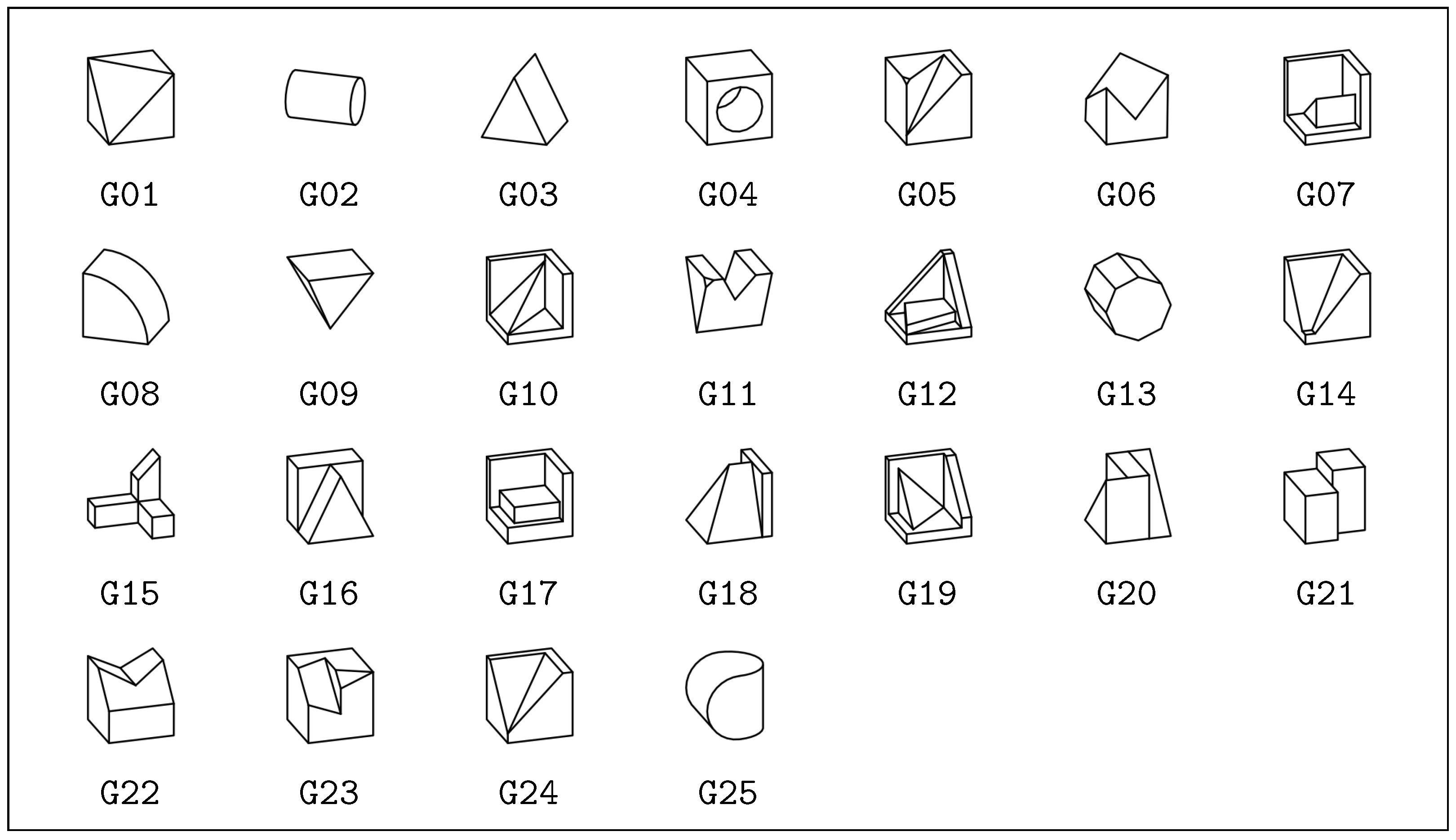
- We have developed additional, manually permuted meshes for each classic mesh. Without using groups G02, G04, G08, and G25, a total number of 205 different manually designed meshes are available (see Figure 1).
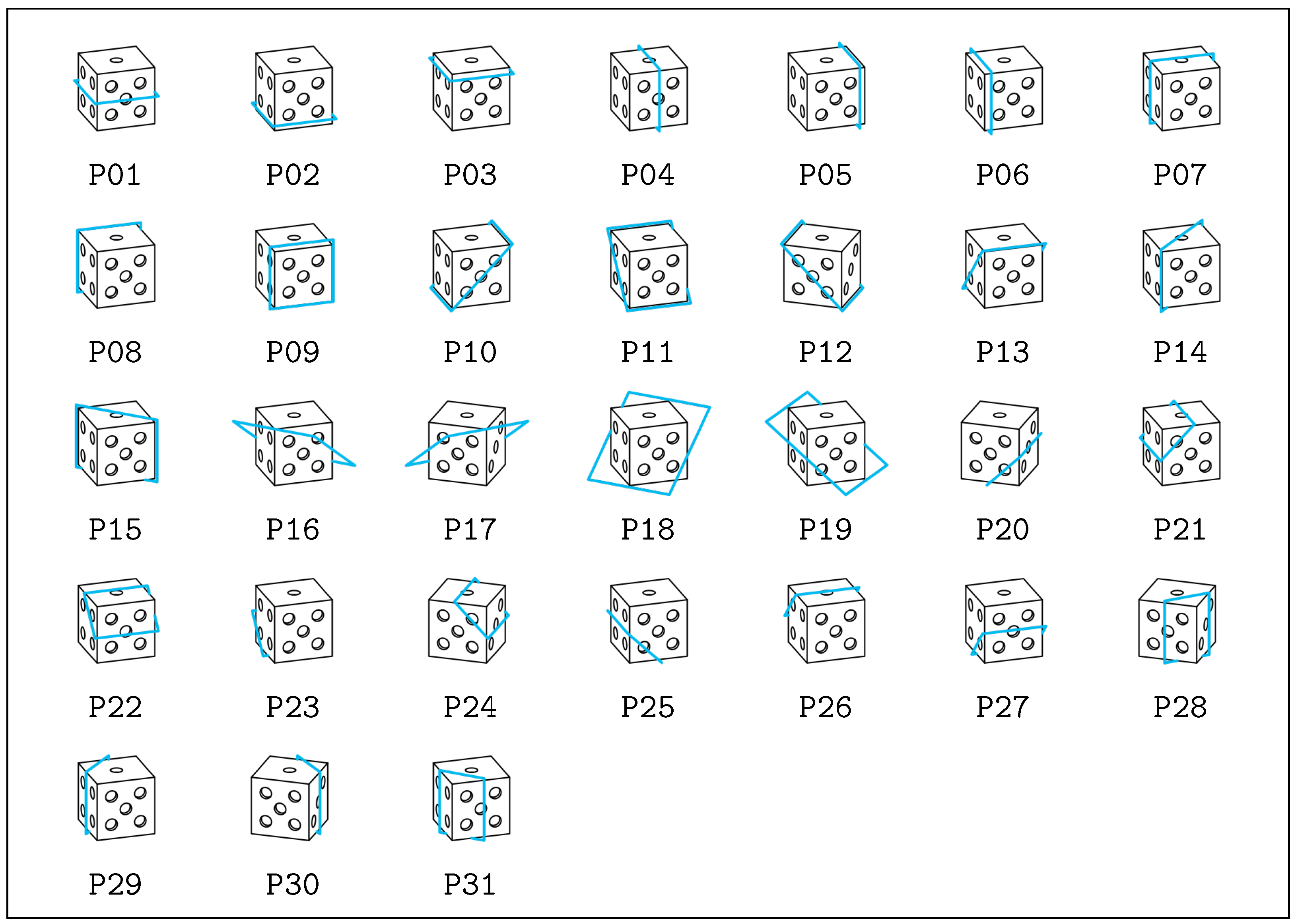
- Thirty-one cutting planes are combined with each mesh (see Figure 2).
- Twenty-four rotation vectors are used to rotate each mesh to each possible orientation using Euler rotation (note that multiple orientations of symmetric shapes can be considered the same).
- Seven scaling vectors yield various meshes, applying a multiplier of 0.7 in one or two dimensions.
We chose two formats to encode our documents. In the case of 2D assets, we prefer SVG (Scalable Vector Format), while in the case of 3D models, our choice was GLB, which is one of the de facto graphical standards and one of the most popular specifications since it is widely supported in different platforms and programming languages. Moreover, it guarantees an efficient representation of all the information about the models. The geometrical features, materials, and textures can be encoded in a single file. Each asset contains a JSON chunk representing the basic information about the asset. The specification supports different methods to encode the binary data; self-contained binary chunks (blobs) are preferred in our case, but it is still possible to refer to external resources using their URLs.
The source code and description of the extended method can be found in our GitHub repository (https://github.com/viskillz/viskillz-blender, accessed on 17 December 2022).
1.3. Our Vision
The dataset with the recently implemented permutation steps contains more than 1 million (1,067,640) scenarios, including small redundancy due to the symmetrical features of the shapes. Focusing on the GLB models for supporting AR, VR, and 3D developments, the assets have a total size of 6,521,971,888 bytes, but the needed disk storage is more than 8 GB in a Windows 11 operating system. Therefore, filtering and processing assets or constructing exercises manually or automatically in an application requires storing the dataset in the database. Thus, a method should be found to allow developers to compress the dataset, making us able to serve content in real time. One possible solution is to find existing compression algorithms; in the case of GLB assets, Draco compression (https://google.github.io/draco/, accessed on 17 December 2022) is a well-known and universal method to compress the assets.
However, different features of the permutation algorithm should be detected in the assets. With the design and development of a domain-specific algorithm, it is possible to achieve a better compression ratio. In this paper, we describe the common features of the assets and introduce an encoding scheme that consists of four levels.
2. Creation and Structure of the Graphical Assets
In this technical section, we introduce the original GLB documents. We focus on the JavaScript Object Notation (JSON) chunk and its properties since this part of the document contains all the properties describing its data chunk. We give a short code snippet for each property, then discuss which values are required or can be omitted in the encoding scheme since they are optional features containing metadata.
Before explaining the JSON chunk, we must mention an unexpected behavior of Blender. If a user creates a custom object or opens a new project and uses the default cube, it does not have a texture or material. However, Blender adds a UV map to each object by default, which behavior cannot be changed. We believe that this behavior affects most of the assets generated using Blender, and it is hard to detect. In this case, the list of textures is empty, and it is not possible to remove the UV map of multiple objects on the UI; designers should adjust each object separately, which takes great effort. This is important because Blender generates a texture for each object, resulting in an empty UV map. It produces a significant overhead since the average size of the related data takes 20–25% of our models (resulting in a total size of 5,070,079,296 bytes without the UV map). Thus, the rest of this paper deals with two scenarios:
- Each model has the UV map due to the behavior of Blender;
- The UV map of each model was removed before the processing.
Our assets were generated with Blender version 3.3. Thus, the description and the calculations are based on the output of this version.
2.1. Properties of the JSON Chunk
2.1.1. Property Asset
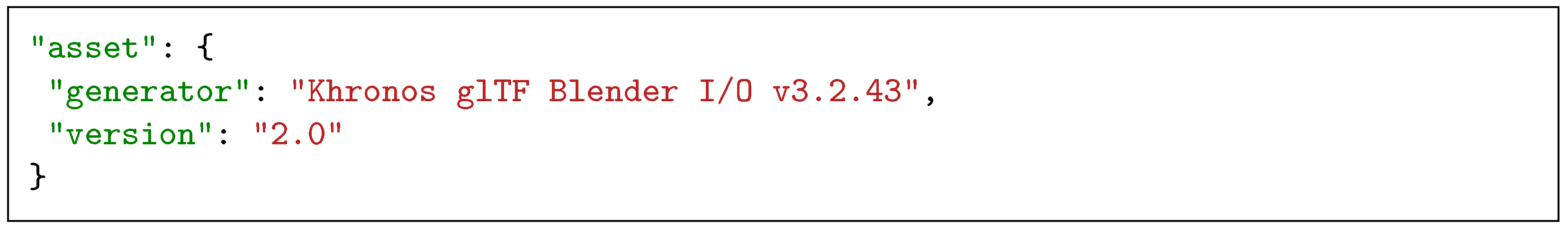
The first property of each JSON document is called the asset, which contains the general attributes of the actual asset, such as its version number. Our assets follow the 2.0 version of the specification [31], and Blender also encodes the name of the generator tool (see Figure 3). Of course, these values are globally identical; none of the assets store different values in these properties. On the other hand, the property generator can be omitted from the documents since this optional attribute does not provide any necessary and meaningful information for the processors.
2.1.2. Properties Scene and Scenes
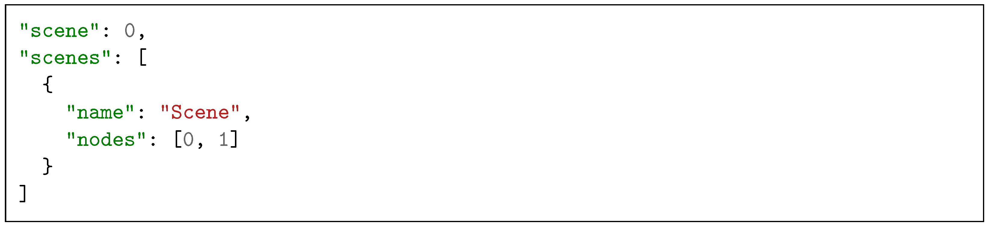
These properties describe the asset’s scenes and their hierarchy. Figure 4 shows that our assets contain a single scene, whose index is stored in the scene property. The specification follows the most practical and classic indexing, which refers to the first element of an array with an index of 0. Thus, the index of our scene is a constant value of 0.
The property scenes describes each scene; thus, this property is a singleton list in our assets. Its first and only element is a Scene object that describes its name and refers to its corresponding node with its ID. The nodes property has a constant value of [0, 1], since each scenario contains a 3D mesh and the representation of the 2D cutting plane. Additionally, they are also being encoded in a strict order. The name attribute is optional, and its value is always the Scene literal. However, they are optional metadata that do not help the parsing and rendering methods of an asset.
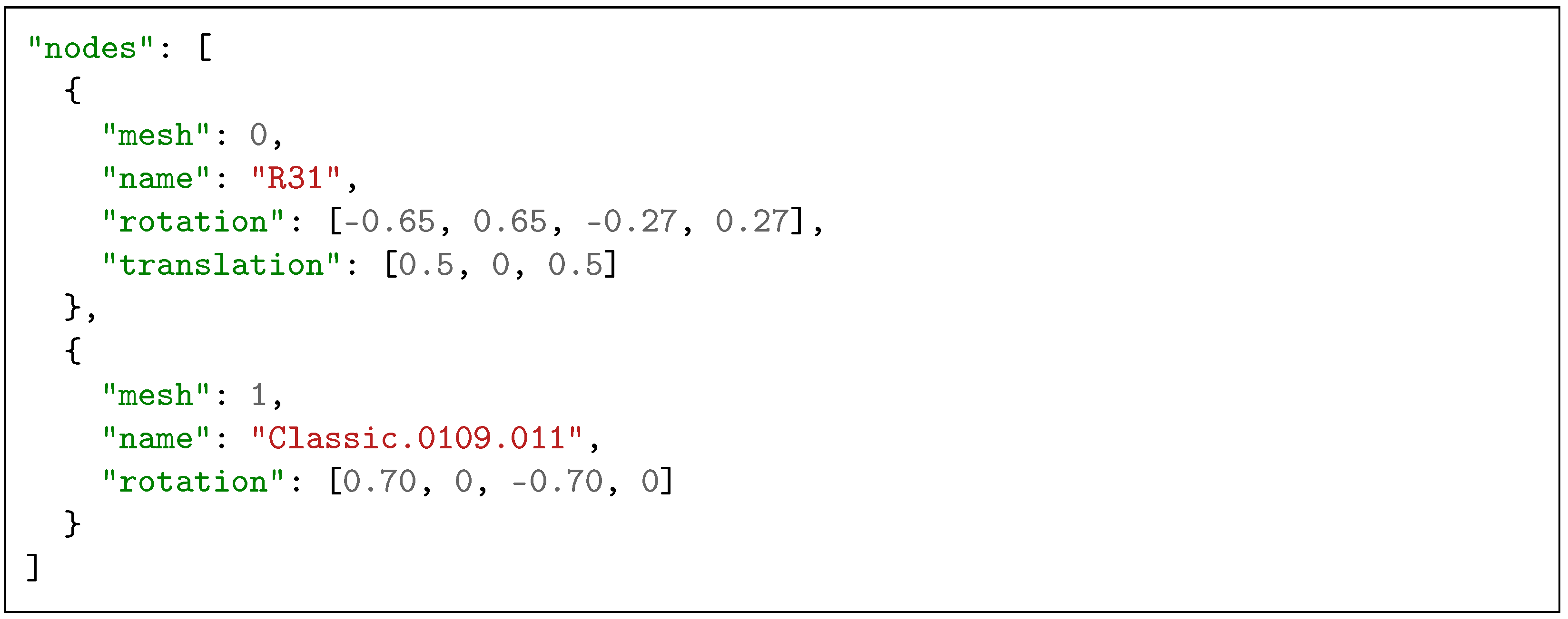
2.1.3. Property Nodes
This property describes the nodes of the asset, which can be interpreted as objects in Blender’s terminology.
In Figure 5, the first object of the array describes the cutting plane, while the second object represents the 3D mesh. The order of the elements—based on the relationship of the corresponding objects in Blender—can be different. However, the naming convention of intersection frames (having IDs starting with R) and 3D meshes (having IDs beginning with the Classic prefix) lets us easily distinguish them in any document. Furthermore, there must be an identical prefix assigned to the cutting planes. Then, the meshes can be named casually. In the case of a document in which the 3D mesh is the first element of the array, we can apply a swap operation on the array, resulting in deterministic order in all the documents. The constant value of the previous scenes property occurred for the same reason reason.
Each object starts with the property mesh, which refers to the corresponding mesh object with its ID. The order of the Node and Mesh objects strictly follow the same order in their arrays. Thus, each of these properties contains the index of the actual Node object (this feature will also be considered in the description of properties having similar sequences in the rest of the document). It is followed by the name property, which contains the name of the corresponding Blender object. They are optional metadata again for which it is not mandatory that they are encoded.
The rest of the properties contain more useful information since the local transforms of each node are listed in these properties. If a transform was not applied in Blender, the matrix_world property of the object differs from the identity matrix. Thus, a GLB file contains the sequence of non-applied transformations in the order of rotation, scale, and translation. They are optional, but each appears if a corresponding transform should be applied to the encoded mesh. The rotation property contains the unit quaternions in order (x,y,z,w), and the scale property contains the scaling factors in (x,y,z) order. In contrast, property translations contain the node’s translation in (x,y,z) order.
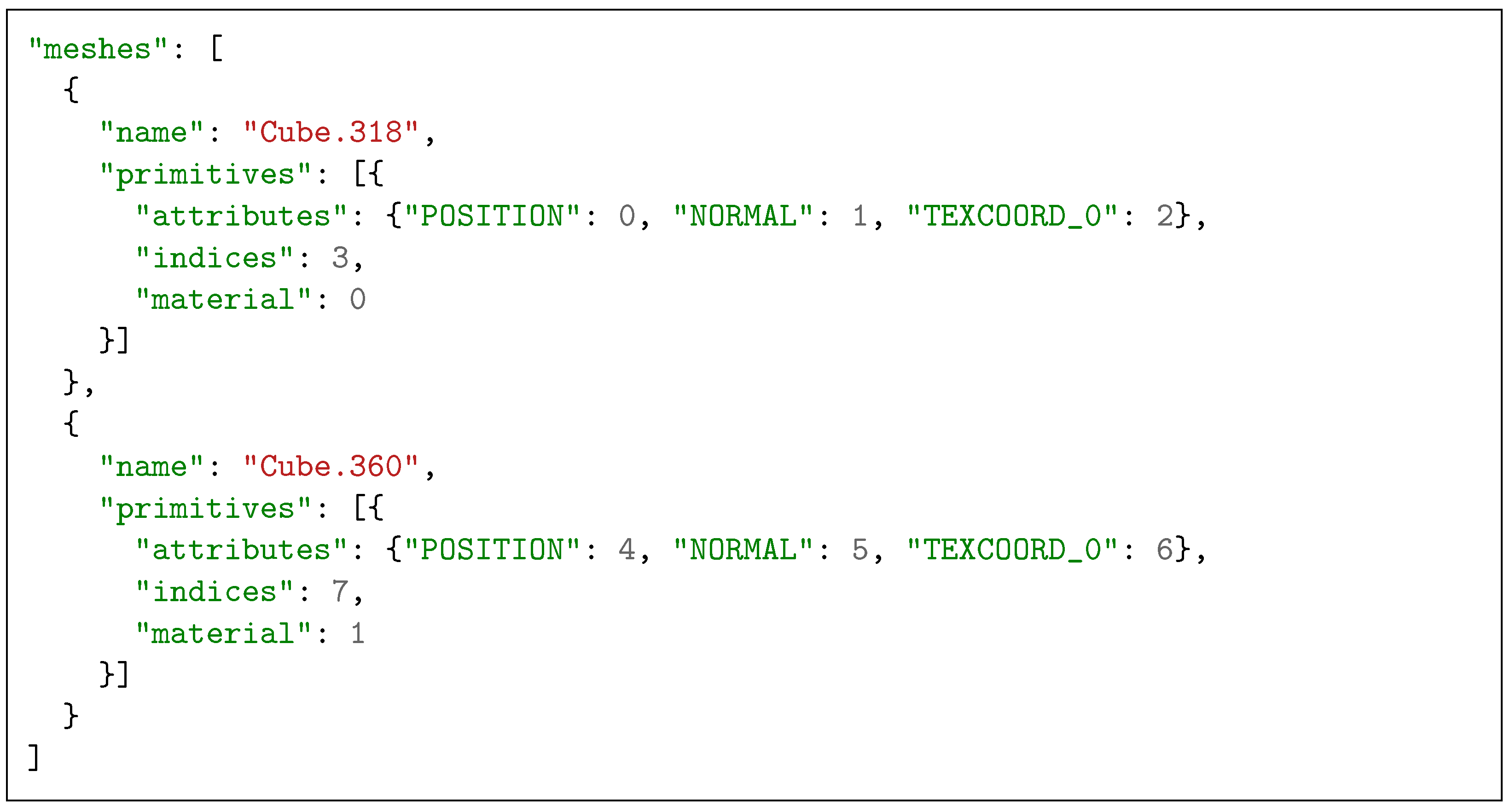
2.1.4. Property Meshes
This property is an array of Mesh objects and connects the nodes to their Accessor objects.
Figure 6 shows that each Mesh object starts with its name property, which are optional metadata again. In our Blender scene, each mesh contains exactly one primitive. Thus, each primitives array is a singleton in the assets. The only Primitive object describes the mapping between the features of the mesh and the Accessor objects, which will tell how the corresponding binary data can be retrieved for the given features. All the values are constant for each scenario because the first four accessors describe the cutting planes, and the last four accessors describe the 3D meshes. Values of the attributes object and the indices property are derived from this feature. Identical materials are applied to our assets, encoded in values of material properties using their indices. These values are also deterministic. The first material belongs to the intersection frame, and the second material belongs to the 3D mesh.
Property meshes is the first in which we can realize the encoded empty textures since property TEXCOORD_0 denotes the Accessor object, which describes the texture of a mesh. As Figure 6 shows, accessors #2 and #6 refer to the textures if they are set; otherwise, each mesh has only two attributes and the indices property (and thus only 3 Accessor objects).
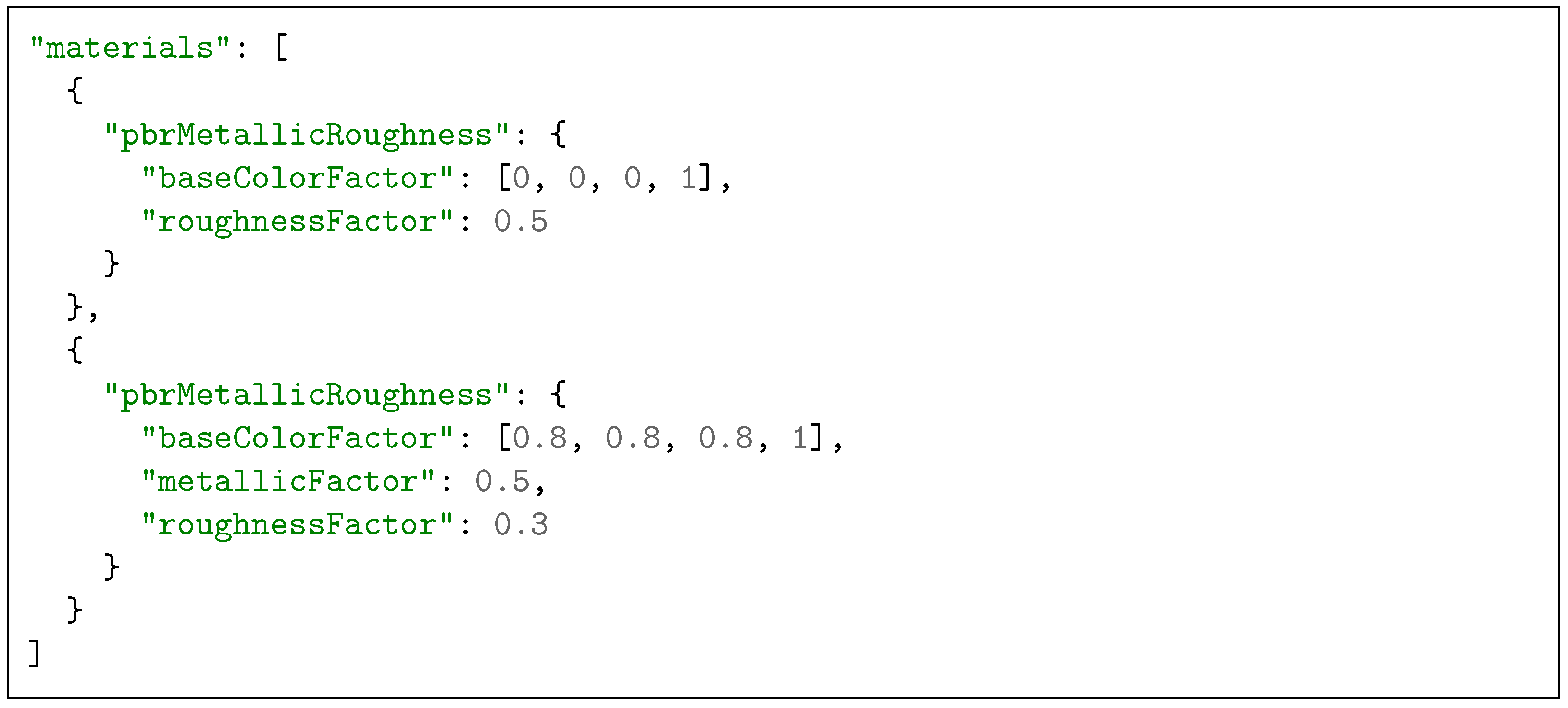
2.1.5. Property Materials
This property contains the materials of each asset.
Figure 7 shows that we use two materials on the meshes of our assets. Various properties can be used in each material to obtain the required appearance of the corresponding meshes. We are serving our cutting planes with a simple, black material. On the other hand, we apply a light gray, metallic material to the 3D meshes; this makes the users able to detect the edges more easily, thanks to the reflections. Thus, the property materials has a globally identical value.
2.1.6. Property Accessors
This property contains the essential high-level properties of the byte buffers, such as their types, sizes (number of elements), and domain range, making processors able to read the content of the binary buffer.
Figure 8 shows that each Accessor object refers to a BufferView object with its ID. This value is identical since each buffer is encoded in the built-in binary chunk. The value of property componentType indicates the datatype of a buffer: Code 5126 denotes an IEEE 754 float type (4 bytes), while code 5123 refers to an unsigned, short integer (2 bytes). Property type tells the structure of the corresponding buffer: Code VEC3 tells that the buffer contains 3-length vectors of the specified datatype, VEC2 means 2-length vectors, while SCALAR means that single values are encoded.
The properties type, componentType, and bufferView have constant values, since textured assets contain eight buffers, while non-textured assets contain six buffers having the same data types in a strict order. The properties min and max only appear in the first buffer of each mesh because it is required for a POSITION accessor and optional in other cases. Accessor objects with indices 2 and 6 refer to textures, encoding pairs of float values.
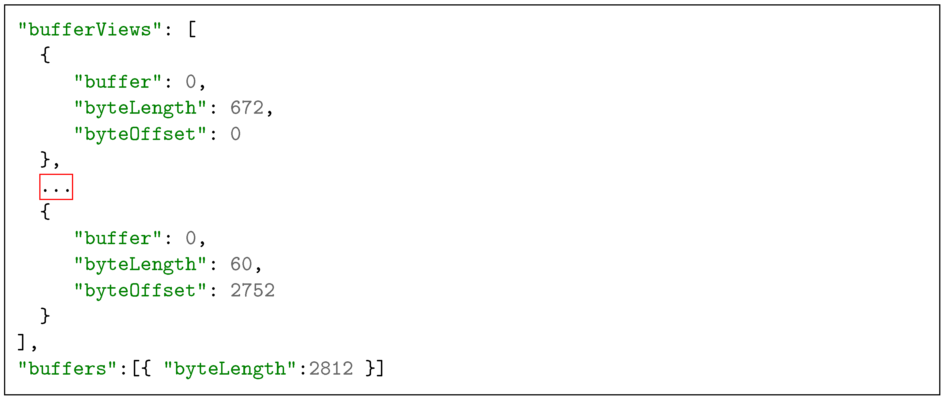
2.1.7. Properties BufferViews and Buffers
Finally, these properties give a low-level description of each binary buffer. Elements of property bufferViews describe a sequence of bytes behind an Accessor, and the property buffers provides the size of each view.
Figure 9 shows properties bufferViews and buffers of our assets. Textured assets have eight BufferView objects, while non-textured assets have six entries in their bufferViews property. Our assets are specific because we do not use external buffers; thus, each feature is encoded in a single, carried, binary chunk of the assets. Thus, the properties of these objects are specific: only the value of the byteLength property needs to be stored since views are sequentially encoded in the binary chunk, and their offsets are deterministic. On the other hand, the buffers property has exactly one entry containing the total length of views in its byteLength property.
2.2. Permutation-Based Features
We have shown that several properties can be eliminated from the encoded files due to the specific features of our assets. Thus, some properties may be omitted from encoded assets, and others can be easily reconstructed from less information. In this section, we mention some important features of our assets.
2.2.1. Property Nodes
Elements of the nodes array describe the frame that denotes the cutting plane, then the shape, which is being intersected by the plane. The permutation step changes their features to yield all the possible combinations in the dataset:
- Each 3D mesh is rotated using 24 different rotation vectors.
- Each 3D mesh is scaled using seven different scaling vectors.
- A total number of 31 cutting planes are combined with each 3D mesh. On the other hand, four different meshes represent a cutting plane. The rest of them can be yielded by applying transformation operators on the set of selected frames.
Thus, we detach the transformations of meshes from individual documents and store them in a global configuration. For example, if a cutting plane appears in multiple assets, the same features should be coded each time in the documents. Moreover, if a shape appears multiple times, its features can also be omitted from the redundant encoding. However, scaling operations were applied in Blender since the Bisect operator deals with local coordinates, and this step serves as a more accessible base for computations. Thus, considering the permutation algorithm, the following properties need to be extracted from documents and should be stored in a global configuration:
- A cleaned Node object for each cutting plane(a total number of 31 objects);
- A cleaned Node object for each rotation vector(a total number of 24 objects).
2.2.2. Property Accessors
The assets contain a deterministic number of Accessor objects: the length of property accessors is 8 in the case of textured assets and 6 in the case of non-textured assets. Their order, property type, and property contentType are identical in both options. The first three or four Accessor objects belong to the cutting plane, and the last three or four Accessor objects belong to the actual shape.
Moreover, accessors of cutting planes can be simplified. The only difference between them appears in the min and max attributes of their POSITION (second) accessor: Accessors of the first 19 cutting planes (numbered from P01 to P19) and the least 12 planes (numbered from P20 to P31) are identical. This feature is derived from the size of the cutting planes: P01-P19 result in the same dimensions on all global axes, while P20-P31 do not satisfy this criterion and result in asymmetric sizes. As a result, only four Accessor objects need to be stored: we chose planes P01, P10, P16, and P20. Furthermore, these accessors can be stored in the global configuration and applied to all scenarios permuted from any 3D shape.
Since the number of possible permutations results from the number of scaled shapes, the number of rotation vectors and the number of intersecting planes, a total number of accessors should be stored to yield the accessors of each permutation of a shape. On the other hand, only the property count of each Accessor object should be kept with the min and max properties of the second accessors individually; other properties have globally identical values.
2.2.3. Properties BufferViews and Buffers
The values of these properties can be computed from the properties of Accessor objects, using their order and properties type, contentType, and length.
2.2.4. Data Chunk
As can be derived from the description of the JSON chunk, binary data are self-stored in each asset, and Accessor and BufferView objects can be used to retrieve a required sub-sequence of the binary encoded data. Now we can examine whether finding a pattern in these byte sequences is possible, as we know that most JSON properties—such as the buffers, bufferViews, and accessors—can be clearly separated into their shape-dependent and plane-dependent components.
The sequence of Accessor objects tells the answer. The first part of each binary chunk belongs to the cutting plane, while the rest contains the binary data of the actual mesh. Thus, the first part of the binary data—like the properties of the JSON document—can be removed from individual assets and stored in a global document. The first 1984 bytes of each buffer belong to the cutting planes; the rest of the bytes belong to the actual shape in the case of textured assets. Otherwise, the first 1536 bytes belong to the cutting plane.
3. Reduced Storage of the Dataset for Efficient Use in Application
In the previous sections, we described the basic features of scenarios. Based on the background knowledge, various data formats can be designed to store the local and global features of assets. In this section, we introduce the multi-level scheme allowing us to reduce the needed storage to store the dataset and encode the information in the most suitable format for the actual use case.
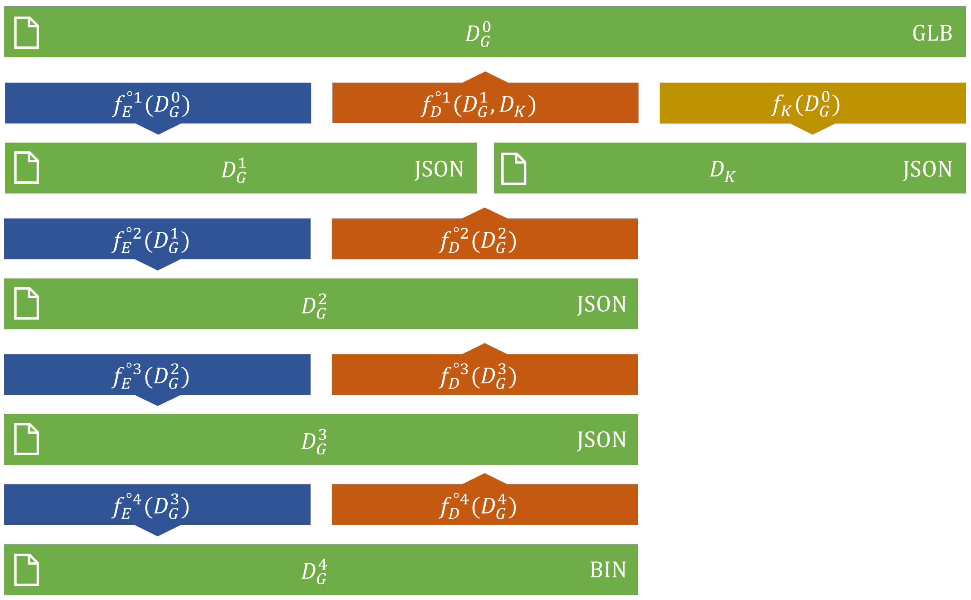
Figure 10 shows that the encoding and decoding steps form a pipeline of individual operations on the dataset; the input of each encoding function is the output of the upper layer, and the input of each decoding function is the output of the lower layer. Each level has its encoding and decoding functions, denoted with and , where subscripts E and D refer to Encoding and Decoding, while superscript refers to the number of the corresponding level (where denotes the original dataset and levels are numbered from 1 to 4 inclusive). Thus, the original assets and encoded documents are noted with , where the optional subscript G notes the ID of the corresponding group. Moreover, documents can be textured or non-textured. Thus, additional letters T and N can be added optionally to the superscripts to distinguish them, resulting in notations and .
3.1. Key Document
Introduce function that extracts the globally identical features from a given dataset, including each property mentioned above, and then encodes them in a JSON document.
The function can be called with any group of assets since the retrieved properties are globally identical. Consequently, this function must be called only once on a dataset, allowing us to retrieve the needed values in each invocation of . Thus, the parameter list of the first decoding function must be extended by introducing another parameter , resulting in the form . The size of the document is 22,958 bytes in the case of textured documents and 19,000 bytes in the case of non-textured documents, using no indentation nor spaces between tokens. On the other hand, the structure of this document can be optimized to achieve a smaller size. However, multiple values should be fetched during the decoding of an asset. Thus, we prefer efficient accessibility to the minimized size of a single document. In this approach, needed values can be easily fetched after reading the document into memory; then, only accessing entries from the dictionary is needed instead of applying transforms on any value.
3.2. First Level
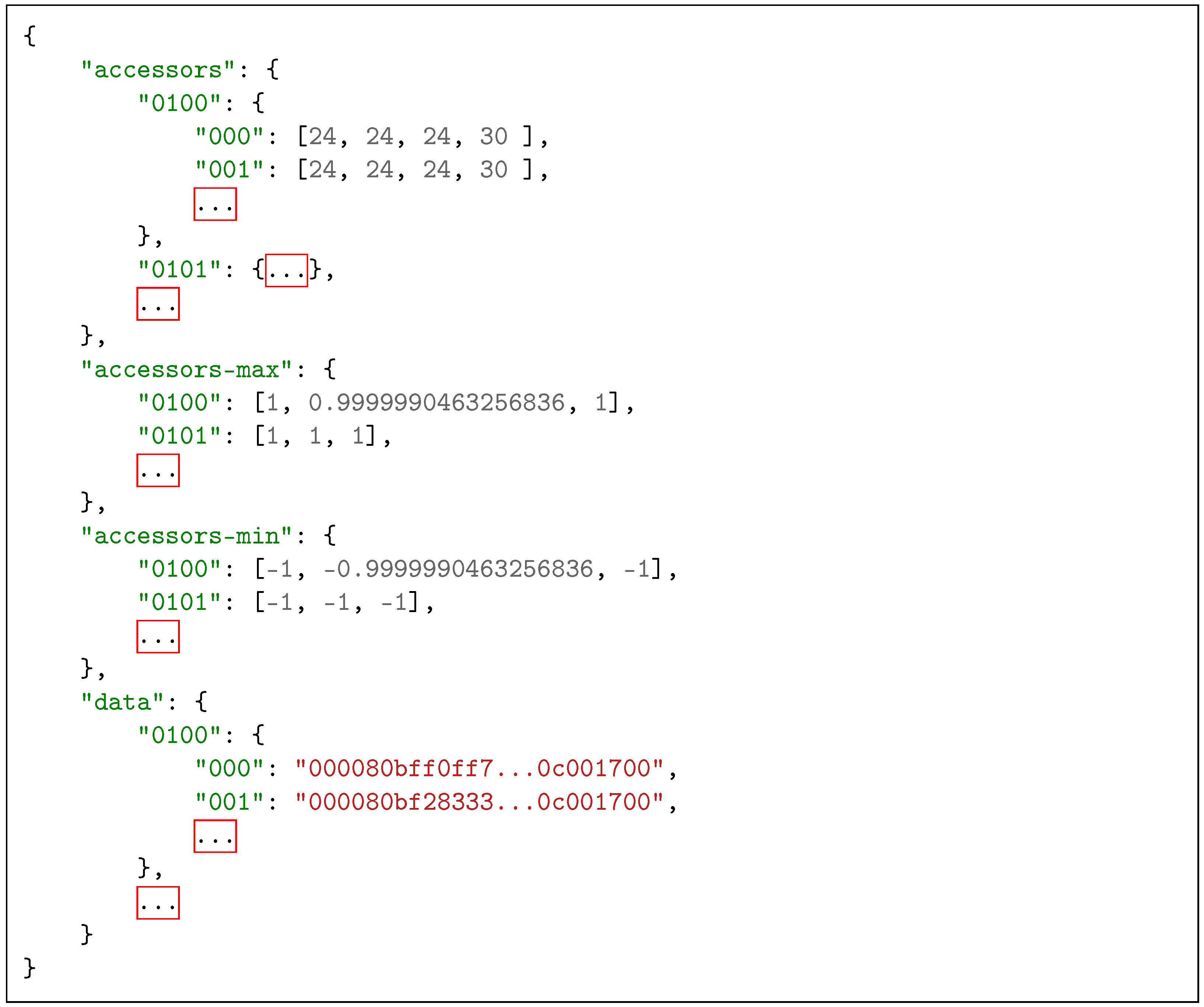
The encoding function consumes a set of original assets that belong to the same group and then returns a JSON document denoted with , containing all the properties that should be stored to reconstruct the original assets with the use of . As Figure 11 suggests, the content of the binary chunk is stored without any processing, so the content of the buffer sequence is encoded as a single series of characters, following their original order. The hexadecimal representation of the bytes was chosen since the numerical types stored in the binary chunk have sizes of 2 or 4 bytes. Thus, an encoding is needed such that each value can be encoded with a different series of characters without padding.
The decoding function reconstructs the original assets of group G by combining the relevant local and global values stored in the properties of and .
With the use of , storage sizes can be reduced by 99.91% in the case of , achieving a compression ratio of 1065 compared to dataset. Both the compression ratio (99.91%) anthe d saved storage size (1077) are similar in the case of and .
3.3. Second Level
The encoding function returns a second-level encoded JSON document . The new document keeps properties accessors-max and accessors-min of but eliminates property accessors by processing and transforming the hexadecimal of the property data.
The idea of the transform operation is to encode each buffer content separately instead of encoding the original continuous sequence of bytes as a single hexadecimal value. As a result, the sliced values of property data in contain information about their lengths, as each original string literal is replaced with a list of string literals. Each list contains four values in the case of and three in the case of . Moreover, observing property data of multiple documents, we can recognize that several subsequences appear multiple times in the lists. This feature is derived from the type of data stored in the GLB documents. The first three buffers have IEEE 754 scalar values in vector types, and the last buffer contains 2-byte unsigned integers. As most of them contain geometric information and our assets have common features, most of the scalars appear multiple times in the same buffer. Thus, the size of can be decreased by collecting the set of unique scalar values in each buffer with lengths of characters in the case of and in the case of . The set of unique character sequences can be used as the keyset of a codebook, which allows us to eliminate the original sequences from the documents, replacing them with their identifiers. We introduce hash function , which returns the index of a scalar value in the sequence of the unique values fetched from the nth buffer . The required compression can be performed by substituting the representation of each scalar value with its corresponding hash value. The keynote behind this operation is that the count of distinct scalar values (and thus each index value) requires fewer digits to be encoded than the original scalar values with representation that is 4 or 8 characters long. Thus, the use of decreases the size of each buffer using 3, 4, 3, and 1 bytes to hash 242, 13,713, 63, and 118 different values of the buffers using their indices. Another possible option could be to collect all the unique scalar values globally and store them in . However, this approach would require different indices for the buffers. Furthermore, in the case of B0, it would require changing the length of the hash values from two digits to four digits. In the case of our dataset, it is better to use shorter hash values and create a codebook for each group. However, another dataset containing shapes with various vertices would require more digits in the hash values. In that case, the global approach would be more efficient.
The decoding function consumes a second-level encoded document and returns the corresponding first-level encoded document (). The function splits the hexadecimal series of hash values encoded in property data and replaces them with the original sequences from property data. As the final step, the function merges the elements of each list of property data and re-adds property accessors to the document containing the size of each buffer.
With the use of , storage sizes can be reduced by 62.02% in the case of , achieving a compression ratio of 2.633 compared to the dataset, 2.804 compared to .
3.4. Third Level
The encoding function consumes a second-level encoded JSON document () and returns a third-level encoded JSON document (). Similarly to function , its output keeps the accessors-max and accessors-min properties of the document but applies a second hash function on the values of property data, where subscript n denotes the index of the buffer.
The hexadecimal values still contain significant redundancy, observing the data properties of documents. The purpose of this feature is simple, as we have already hashed each scalar value, but the first three buffers contain vectors of types VEC3, VEC3, and VEC2. Not just the same scalar values, but the same vectors appear multiple times in the original sequences. The first and second buffers contain triplets of float values, while the third vector (that encodes the textures) contains integer pairs. Thus, the statistical features of the subsequences can be analyzed again, verifying that several triples and pairs of hash values appear multiple times. Using decreases the size of the first three buffers using 2, 4, and 1 byte(s) to hash 789, 1179, and 82 different values of the buffers using their indices.
The decoding function consumes a third-level encoded JSON document () and returns a second-level encoded JSON document (). Similarly to function , it splits the hexadecimal sequences of property data, replaces the hash values with the original values from property data-cb-byte-2, and then joins the strings. Finally, property data-cb-byte-2 is removed to retrieve format .
By adding the codebook as a property data-cb-byte-2 and applying function on property data, storage sizes can be reduced by 37.89% in the case of textured documents, achieving a compression ratio of 1.610 compared to the dataset and 4034 compared to dataset. The values are similar in the case of the non-textured dataset.
3.5. Fourth Level
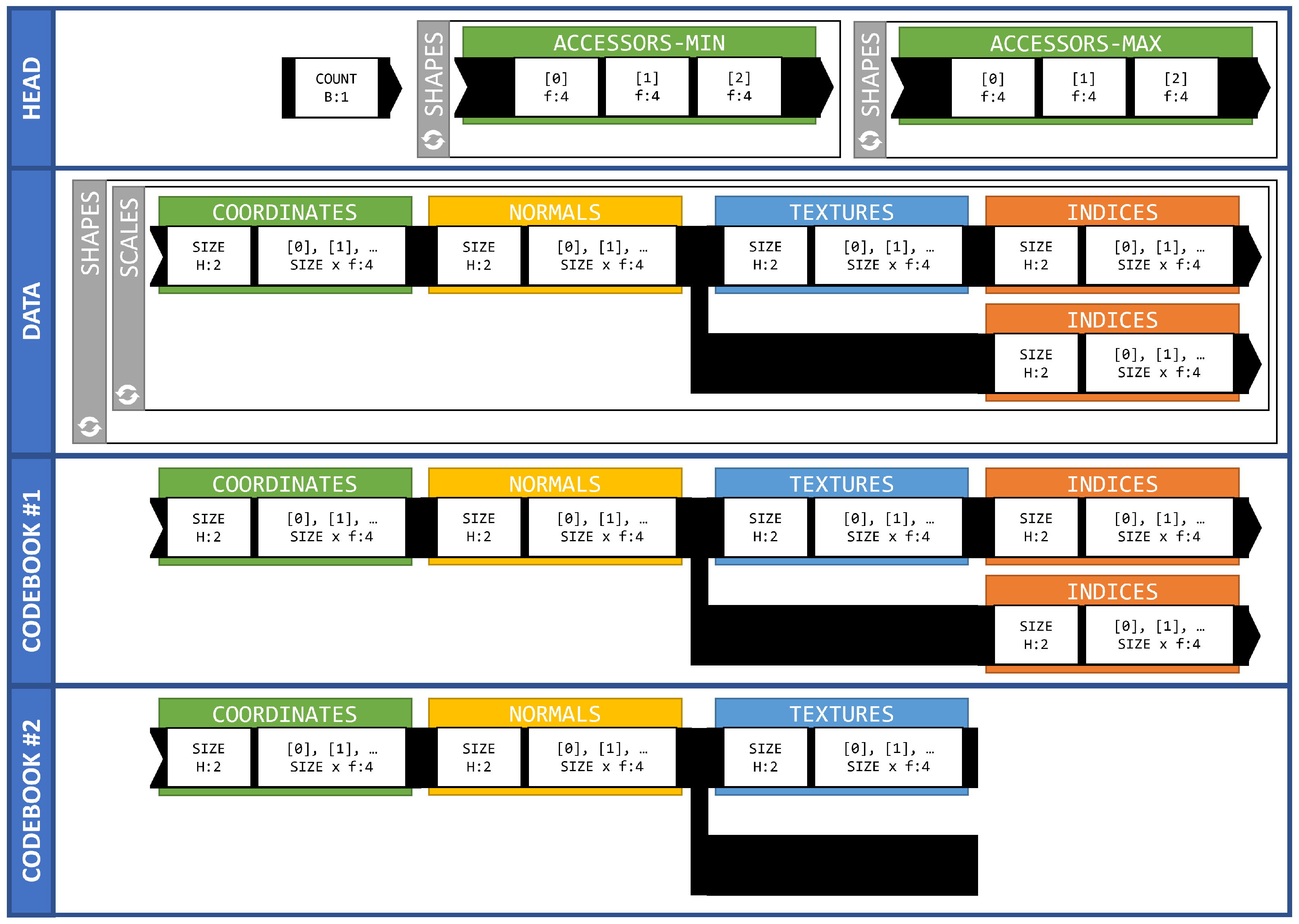
All the previous encoding functions returned valid JSON documents. JSON documents have a lightweight syntax and much less overhead than other formats, such as XML. However, the size of the dataset can be reduced by introducing a binary format instead of a text format. This approach eliminates all tokens of JSON syntax, and our identifiers, as well as the property data, can be encoded as a sequence of bytes instead of hexadecimal character sequences. Moreover, floating numbers in JSON documents are encoded using multiple precision digits but can be encoded using IEEE 754 types. Thus, the encoding function encodes the properties of and decreases the size of the dataset using binary encoding. Figure 12 describes the binary format of and documents.
With the use of the binary encoding, storage sizes can be reduced by 53.15% in the case of textured documents, achieving a compression ratio of 2.134 compared to the dataset and 9634 compared to the dataset. The values are similar in the case of the non-textured dataset.
3.6. Evaluation
3.6.1. Verification
As a first approach, it seems evident that the encoding and decoding algorithms can be verified by encoding and decoding all the assets, then comparing the original and the retrieved files bitwise. However, the bitwise equality of the original and the decoded dataset cannot be guaranteed due to the use of IEEE 754 types. As Figure 11 shows, the raw output of Blender already contains precision errors that can be derived primarily from the use of type IEEE 754 as a sequence of rotation, and scale operations have been applied on most of the assets in Blender.
- Each calculation with an IEEE 754 type increases the probability of a higher error in the result.
- Moreover, the original mesh is designed manually. Thus, designers may make minor errors in setting the coordinates of vertices. Consequently, minor errors occur in the bytes of the data chunk and the values of the JSON chunk.
- Finally, our decoding algorithm applies a multiplication on the min and max properties of Accessor objects to simulate the scaling operation.
If an error occurs in the data chunk, the equality of the file sizes can be guaranteed. However, if a value of the JSON chunk is represented with a precision error, the file size changes. Thus, a comparison method should be implemented, and in using it, the verification can be performed:
- The properties of their JSON chunks should be compared recursively. In the case of floating values, their difference should be above a given threshold . Objects must contain the same key-value pairs, while the order of the elements in two arrays should also be the same.
- The binary chunks can be compared bitwise, except the sequences that belong to a buffer using floating values. In that case, the comparison must be performed using the given threshold .
- Only globally unique metadata (such as property asset) can be reconstructed and checked since the algorithm does not code any metadata in but in .
The comparison can be formed on the dataset using , which is an acceptable value for type IEEE 754.
3.6.2. Analysis
We have already calculated the compression ratio and saved disk space of each encoding level in the description of each encoding function using the textured and non-textured versions of the dataset. However, the runtime of every function should be measured to determine whether the method is acceptable in practice. The aim of the compression is to decrease the size of the dataset, making the storage in file systems and databases possible or easier. Thus, original assets should be decoded without requiring time-consuming calculations, enabling applications to serve content online. Table 1 shows the time complexity of each decoding function, including all the previous decoding functions (that need to be executed) and I/O operations.
During the analysis, we found that the features of the encoding scheme offer an alternate process for yielding the dataset from Blender, decreasing the runtime significantly:
- Export only the subset of assets from Blender, which is required as an input of and . Denote the set of assets with .
- Create with function call .
- Encode each group to retrieve with a function call .
- Decode each document to retrieve the full dataset with a function call .
As Table 2 shows, the original exporting process of Blender requires an average of 33,886 s. On the other hand, the exporting process of the subset requires only an average of 478.1459 s; the encoding process needs 0.2605 s. Finally, the decoding process needs an average of 498.7475 s. Thus, the alternate process requires an average of 977.1520 s instead of Blender’s 33,886 s, resulting in 2.8836% of the original runtime by eliminating geometric computations and permuting the assets without using Blender.
3.6.3. Remarks
- Each calculation was performed on a Zenbook UX433FA-A5082T notebook with an SSD and OS Windows 11.
- During the measurements, only our Blender script or standalone Python scripts were executed on the computer. All the other non-essential processes had been stopped, including Windows Defender.
- The Blender script was executed using the built-in interpreter of Blender 3.3, using our wrapper script.
- The wrapper script and encoding process were interpreted with Python version 3.10.6 in a Miniconda 4.14.0 environment.
- Each mentioned runtime is an average of processes in the case of our Blender script, and five processes in the case of our encoding and decoding functions.
- A pre-processing step was executed before the encoding process to guarantee that all the shapes had the same materials without precision errors that affected the calculations. The material shown in Figure 7 has been added to all the assets in this step.
3.7. Applications
The ultimate aim of our research was to create an easy-to-use open-access database and application framework supporting students in their learning process to acquire more thorough spatial skills. In this process, the application of augmented reality is a great asset to understand spatial relations better, but these tools typically require powerful hardware and large storage capacity; none of them are available in students’ cell phones. Moreover, the lack of a large number of tasks is a further limitation to effective skill development. These bottlenecks are effectively resolved by our contribution described above.
The encoding scheme presented in the previous chapter is already used in our applications viSkillz Browser and viSkillz Quiz. The app viSkillz Browser (see Figure 13) allows users to browse the raw output of the permutation algorithm, while the application viSkillz Quiz combines a survey and MCT exercises. In addition, both of the applications offer 3D models to their users, encoded with the proposed encoding algorithm and stored in a MongoDB database. More details about the applications can be found in our previous publication [36]. Moreover, the applications can be accessed via the addresses https://viskillz.inf.unideb.hu/browser and https://viskillz.inf.unideb.hu/quiz, accessed on 17 December 2022. A sample quiz can be launched using the token EN. The development of further apps in several platforms is available for anyone using the 3D data (see, e.g., Figure 13, Figure 14 and Figure 15).
4. Conclusions
In this paper, we dealt with processing a dataset containing assets of Mental Cutting Test exercises. MCT is one of the most popular tests through which spatial skills can be improved and evaluated; however, designing a significant number of scenarios is a time-consuming process. Thus, we have developed our script-aided process in the last few years, which applies permutation steps automatically on the manually designed meshes. The permutations include scaling, rotation, and using a set of cutting planes. However, it is not apparent how the whole dataset can be stored in a database without limitations, since the dataset size exceeds 6 GB.
As a result of this paper, we introduced an encoding scheme that processes the GLB assets and retrieves their common properties. The basis of the algorithm is that the various permutation factors can be detected in the byte sequences of the assets; thus, it is not required to store each asset, making an application able to serve them. Our algorithm can encode and decode the dataset using , achieving saved disk space of and a compression ratio of over .
Moreover, we can avoid executing the entire generation process in Blender, including time-consuming transform calculations. As an alternate solution, a subset of the original assets needs to be generated, from which all the required information can be retrieved using our encoding functions. Then, the whole dataset can be restored using the decoding functions, requiring only of the original runtime.
Finally, using our encoding scheme, users can detach materials from the geometric data of their assets since materials are stored in . Various versions of can be created, containing different materials. Thus, different assets can be retrieved for different purposes. This approach follows the excellent practice of storing documents and styles separately using other technologies such as HTML and CSS.
Based on the common features of various spatial exercises, similar encoding schemes can be designed to minimize the size of a dataset and offer better efficiency in the development process of applications for the purpose of effectively improving spatial skills, even with limited hardware and storage capacity.
Author Contributions
Conceptualization: R.T., M.H. and M.Z.; Methodology: R.T., M.H. and M.Z.; Software: R.T.; Formal analysis and investigation: R.T., M.H. and M.Z.; Writing—original draft preparation: R.T.; Writing—review and editing: M.H. and M.Z.; Funding acquisition: R.T.; Resources: M.H. and M.Z. Supervision: M.H. and M.Z. All authors have read and agreed to the published version of the manuscript.
Funding
Supported by the ÚNKP-22-3 New National Excellence Program of the Ministry for Culture and Innovation from the source of the National Research, Development and Innovation Fund. Any opinions, findings, and conclusions or recommendations expressed in this material are those of the authors and do not necessarily reflect the views of the funders.
Institutional Review Board Statement
Not applicable.
Informed Consent Statement
Not applicable.
Data Availability Statement
The source code and documentation of the original, script-aided process and the Blender project containing the meshes can be found in our GitHub repository viskillz-blender: https://github.com/viskillz/viskillz-blender, accessed on 17 December 2022. The source code and documentation of the encoding and decoding functions can be found in our GitHub repository viskillz-glb: https://github.com/viskillz/viskillz-glb, accessed on 17 December 2022.
Acknowledgments
Thank you for Balázs Pintér providing the screenshots of their iOS application developed as a thesis project.
Conflicts of Interest
The authors declare no conflict of interest.
Abbreviations
The following abbreviations are used in this manuscript:
| MCT | Mental Cutting Test |
| GLB | GL Transmission Format Binary file |
References
- Bohlmann, N.; Benölken, R. Complex Tasks: Potentials and Pitfalls. Mathematics 2020, 8, 1780. [Google Scholar] [CrossRef]
- Bishop, A.J. Spatial abilities and mathematics education—A review. Educ. Stud. Math. 1980, 11, 257–269. [Google Scholar] [CrossRef]
- Tosto, M.G.; Hanscombe, K.B.; Haworth, C.M.; Davis, O.S.; Petrill, S.A.; Dale, P.S.; Malykh, S.; Plomin, R.; Kovas, Y. Why do spatial abilities predict mathematical performance? Dev. Sci. 2014, 17, 462–470. [Google Scholar] [CrossRef] [PubMed]
- Cole, M.; Wilhelm, J.; Vaught, B.M.M.; Fish, C.; Fish, H. The Relationship between Spatial Ability and the Conservation of Matter in Middle School. Educ. Sci. 2021, 11, 4. [Google Scholar] [CrossRef]
- Zimmermann, W.; Cunningham, S. (Eds.) Visualization in Teaching and Learning Mathematics; Mathematical Association of America: Washington, DC, USA, 1991. [Google Scholar]
- Presmeg, N. Visualization and Learning in Mathematics Education. In Proceedings of the Encyclopedia of Mathematics Education; Springer International Publishing: Cham, Switzerland, 2020; pp. 900–904. [Google Scholar]
- Presmeg, N. Spatial Abilities Research as a Foundation for Visualization in Teaching and Learning Mathematics. In Proceedings of the Critical Issues in Mathematics Education; Springer: Boston, MA, USA, 2008; pp. 83–95. [Google Scholar]
- Gerber, A. (Ed.) Spatial Abilities. A Workbook for Students of Architecture; Birkhauser Verlag GmbH: Basel, Switzerland, 2020. [Google Scholar]
- Katsioloudis, P.; Bairaktarova, D. Impacts of Scent on Mental Cutting Ability for Industrial and Engineering Technology Students as Measured Through a Sectional View Drawing. In Proceedings of the Spatial Cognition XII; Šķilters, J., Newcombe, N.S., Uttal, D., Eds.; Springer: Cham, Switzerland, 2020; pp. 322–334. [Google Scholar]
- Estapa, A.; Nadolny, L. The effect of an augmented reality enhanced mathematics lesson on student achievement and motivation. J. Stem Educ. 2015, 16, 40–48. [Google Scholar]
- Chen, Y. Effect of mobile augmented reality on learning performance, motivation, and math anxiety in a math course. J. Educ. Comput. Res. 2019, 57, 1695–1722. [Google Scholar] [CrossRef]
- del Cerro Velázquez, F.; Morales Méndez, G. Application in Augmented Reality for Learning Mathematical Functions: A Study for the Development of Spatial Intelligence in Secondary Education Students. Mathematics 2021, 9, 369. [Google Scholar] [CrossRef]
- Petrov, P.D.; Atanasova, T.V. The Effect of Augmented Reality on Students’ Learning Performance in Stem Education. Information 2020, 11, 209. [Google Scholar] [CrossRef] [Green Version]
- Flores-Bascuñana, M.; Diago, P.D.; Villena-Taranilla, R.; Yáñez, D.F. On Augmented Reality for the learning of 3D-geometric contents: A preliminary exploratory study with 6-Grade primary students. Educ. Sci. 2020, 10, 4. [Google Scholar] [CrossRef] [Green Version]
- Suselo, T.; Wünsche, B.C.; Luxton-Reilly, A. Using Mobile Augmented Reality for Teaching 3D Transformations. In Proceedings of the 52nd ACM Technical Symposium on Computer Science Education, Virtual Event, 13–20 March 2021; pp. 872–878. [Google Scholar]
- CEEB Special Aptitude Test in Spatial Relations; College Entrance Examination Board: New York, NY, USA, 1939.
- Bölcskei, A.; Gál-Kállay, S.; Kovács, A.Z.; Sörös, C. Development of Spatial Abilities of Architectural and Civil Engineering Students in the Light of the Mental Cutting Test. J. Geom. Graph. 2012, 16, 103–115. [Google Scholar]
- Šipuš, Ž.M.; Cižmešija, A. Spatial ability of students of mathematics education in Croatia evaluated by the Mental Cutting Test. Ann. Math. Informaticae 2012, 40, 203–216. [Google Scholar]
- Németh, B.; Sörös, C.; Hoffmann, M. Typical mistakes in Mental Cutting Test and their consequences in gender differences. Teach. Math. Comput. Sci. 2007, 5, 385–392. [Google Scholar] [CrossRef]
- Németh, B.; Hoffmann, M. Gender differences in spatial visualization among engineering students. In Proceedings of the Annales Mathematicae et Informaticae; Institute of Mathematics and Informatics of Eszterházy Károly University: Eger, Hungary, 2006; pp. 169–174. [Google Scholar]
- Ballatore, M.G.; Duffy, G.; Sorby, S.; Tabacco, A. SAperI: Approaching Gender Gap Using Spatial Ability Training Week in High-School Context. In Proceedings of the Eighth International Conference on Technological Ecosystems for Enhancing Multiculturality, Salamanca, Spain, 21–23 October 2020; TEEM’20. pp. 142–148. [Google Scholar] [CrossRef]
- Tóth, R.; Zichar, M.; Hoffmann, M. Improving and Measuring Spatial Skills with Augmented Reality and Gamification. In Proceedings of the International Conference on Geometry and Graphics, Sao Paulo, Brazil, 18–22 January 2021; pp. 755–764. [Google Scholar]
- Guzsvinecz, T.; Szeles, M.; Perge, E.; Sik-Lanyi, C. Preparing spatial ability tests in a virtual reality application. In Proceedings of the 2019 10th IEEE International Conference on Cognitive Infocommunications (CogInfoCom), Naples, Italy, 23–25 October 2019; pp. 363–368. [Google Scholar]
- Tóth, R.; Zichar, M.; Hoffmann, M. Gamified Mental Cutting Test for enhancing spatial skills. In Proceedings of the 2020 11th IEEE International Conference on Cognitive Infocommunications (CogInfoCom), Mariehamn, Finland, 23–25 September 2020; pp. 299–304. [Google Scholar]
- Rizzo, A.A.; Buckwalter, J.G.; Neumann, U.; Kesselman, C.; Thiébaux, M.; Larson, P.; van Rooyen, A. The virtual reality mental rotation spatial skills project. Cyberpsychol. Behav. 1998, 1, 113–119. [Google Scholar] [CrossRef]
- Lochhead, I.; Hedley, N.; Çöltekin, A.; Fisher, B. The Immersive Mental Rotations Test: Evaluating Spatial Ability in Virtual Reality. Front. Virtual Real. 2022, 3. [Google Scholar] [CrossRef]
- Hartman, N.W.; Connolly, P.E.; Gilger, J.W.; Bertoline, G.R.; Heisler, J. Virtual reality-based spatial skills assessment and its role in computer graphics education. In Proceedings of the ACM SIGGRAPH’06 Proceedings, Boston, MA, USA, 30–31 July 2006; p. 46. [Google Scholar]
- Safadel, P.; White, D. Effectiveness of computer-generated virtual reality (VR) in learning and teaching environments with spatial frameworks. Appl. Sci. 2020, 10, 5438. [Google Scholar] [CrossRef]
- Saredakis, D.; Szpak, A.; Birckhead, B.; Keage, H.A.D.; Rizzo, A.; Loetscher, T. Factors associated with virtual reality sickness in head-mounted displays: A systematic review and meta-analysis. Front. Hum. Neurosci. 2020, 14, 96. [Google Scholar] [CrossRef] [PubMed] [Green Version]
- Chang, E.; Kim, H.T.; Yoo, B. Virtual reality sickness: A review of causes and measurements. Int. J. Hum. Comput. Interact. 2020, 36, 1658–1682. [Google Scholar] [CrossRef]
- The Khronos® 3D Formats Working Group. GlTF™ 2.0 Specification-Version 2.0.1. 2021. Available online: https://registry.khronos.org/glTF/specs/2.0/glTF-2.0.html (accessed on 11 September 2022).
- Fedyukov, M. IEEE Industry Connections (IEEE-IC) File Format Recommendations for 3D Body Model Processing; IEEE: New York, NY, USA, 2019; pp. 1–38. [Google Scholar]
- Yang, Q.; Dong, X.; Cao, X.; Ma, Y. Adaptive compression of 3D models for mobile web apps. In Proceedings of the 20th Annual International Conference on Mobile Systems, Applications and Services, Portland, OR, USA, 27 June–1 July 2022. [Google Scholar]
- Possemiers, A.L.; Lee, I. Fast OBJ file importing and parsing in Cuda. Comput. Vis. Media 2015, 1, 229–238. [Google Scholar] [CrossRef] [Green Version]
- Tuker, C. Training Spatial Skills with Virtual Reality and Augmented Reality. In Encyclopedia of Computer Graphics and Games; Springer International Publishing: Cham, Switzerland, 2018; pp. 1–9. [Google Scholar] [CrossRef]
- Tóth, R.; Tóth, B.; Zichar, M.; Fazekas, A.; Hoffmann, M. Educational Applications to Support the Teaching and Learning of Mental Cutting Test Exercises. In Proceedings of the ICGG 2022–Proceedings of the 20th International Conference on Geometry and Graphics, Sao Paulo, Brazil, 15–19 August 2022; pp. 928–938. [Google Scholar] [CrossRef]
- Tóth, R. Script-aided generation of Mental Cutting Test exercises using Blender. Ann. Math. Inform. 2021, 54, 147–161. [Google Scholar] [CrossRef]
- Python Software Foundation. Struct—Interpret Bytes as Packed Binary Data—Python 3.10.7 Documentation. 2022. Available online: https://docs.python.org/3/library/struct.html (accessed on 11 September 2022).
Figure 1.
A set of shapes abstracted and reconstructed from the well-known sheet of MCT exercises.

Figure 2.
The set of intersection planes demonstrated in a simple cube that were used to permute the scenarios.
Figure 2.
The set of intersection planes demonstrated in a simple cube that were used to permute the scenarios.

Figure 3.
Property asset of the JSON chunk in an MCT asset.

Figure 4.
Properties scene and scenes of the JSON chunk in an MCT asset.

Figure 5.
Property nodes of the JSON chunk in an MCT asset.

Figure 6.
Property meshes of the JSON chunk in an MCT asset.

Figure 7.
Property materials of the JSON chunk in an MCT asset.

Figure 8.
Properties accessors, bufferViews and buffers of the JSON chunk in an MCT asset.

Figure 9.
Properties accessors, bufferViews and buffers of the JSON chunk in an MCT asset.

Figure 10.
The multi-level encoding scheme.

Figure 11.
The structure of , with four numbers in each array of the property accessors. Precision errors can be also detected in the scalars of properties accessors-max and accessors-min.
Figure 11.
The structure of , with four numbers in each array of the property accessors. Precision errors can be also detected in the scalars of properties accessors-max and accessors-min.

Figure 12.
The structure of and binary files. Notations of types are derived from the struct module of Python [38].
Figure 12.
The structure of and binary files. Notations of types are derived from the struct module of Python [38].

Figure 13.
Screenshot of our viSkillz Browser application, storing and serving our models using the proposed method.
Figure 13.
Screenshot of our viSkillz Browser application, storing and serving our models using the proposed method.

Figure 14.
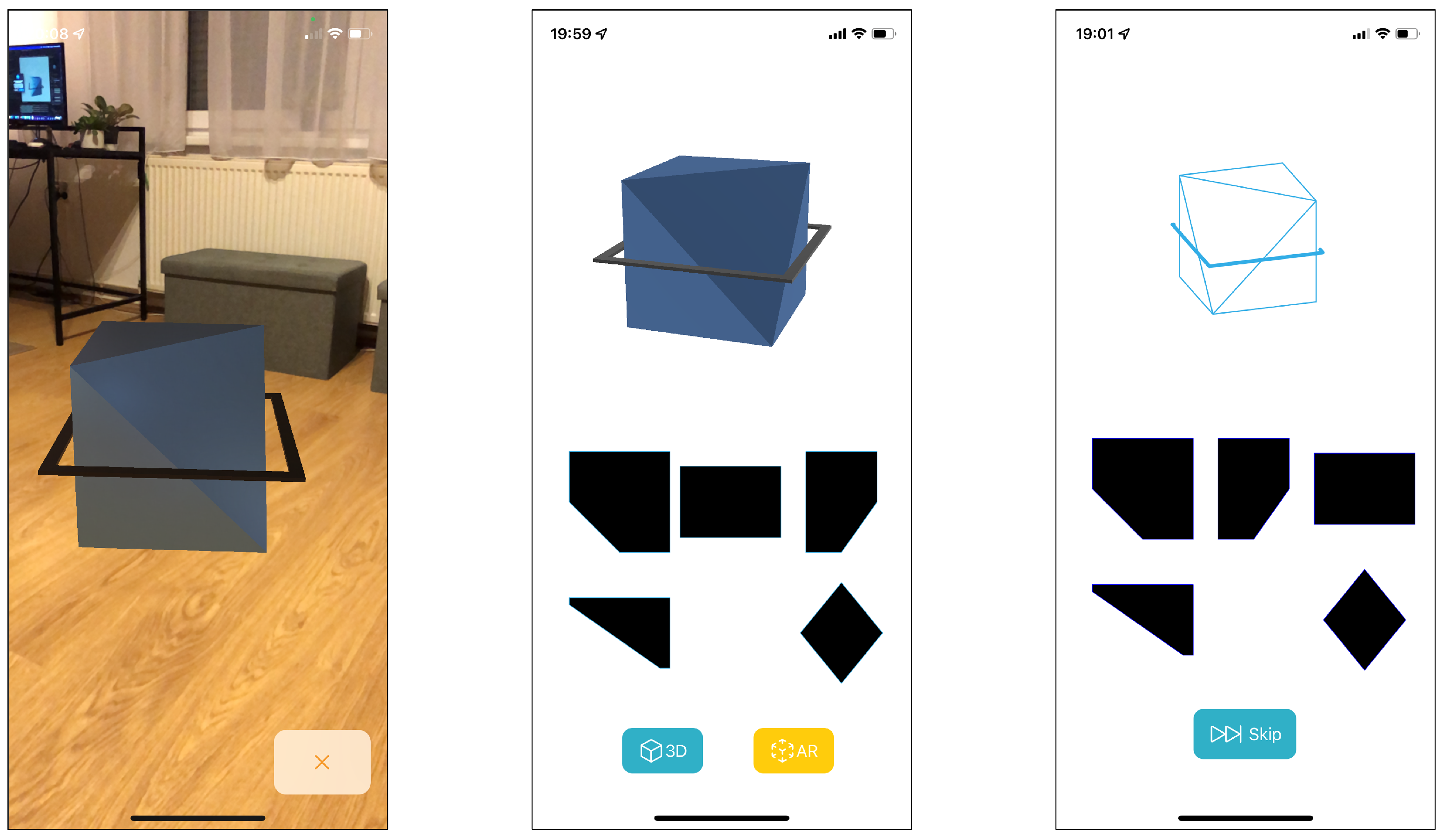
Screenshots of an iOS application using our API.

Figure 15.
Screenshot of the built-in 3D viewer of the Windows 11 operating system. With the application, it is possible to display the assets, modify them, or interact with them.
Figure 15.
Screenshot of the built-in 3D viewer of the Windows 11 operating system. With the application, it is possible to display the assets, modify them, or interact with them.


Table 1.
Decoding time in seconds of each function.
| Group | ||||||||
|---|---|---|---|---|---|---|---|---|
| 01 | 23.89 | 24.38 | 23.98 | 24.47 | 22.89 | 22.71 | 23.48 | 23.88 |
| 03 | 24.08 | 23.90 | 23.75 | 24.43 | 22.99 | 22.97 | 23.42 | 23.51 |
| 05 | 19.38 | 19.13 | 19.64 | 19.27 | 18.67 | 18.38 | 19.18 | 18.75 |
| 06 | 19.52 | 19.50 | 19.90 | 19.17 | 18.66 | 18.50 | 19.30 | 19.04 |
| 07 | 24.35 | 24.65 | 25.39 | 24.27 | 22.70 | 23.34 | 23.67 | 23.67 |
| 09 | 24.29 | 24.87 | 24.65 | 24.80 | 23.23 | 23.18 | 23.68 | 23.84 |
| 10 | 24.88 | 24.93 | 24.63 | 24.26 | 23.53 | 23.01 | 24.04 | 24.09 |
| 11 | 27.13 | 26.86 | 27.61 | 26.35 | 25.76 | 26.15 | 26.38 | 26.49 |
| 12 | 24.28 | 24.83 | 24.43 | 24.46 | 23.58 | 23.47 | 23.92 | 23.96 |
| 13 | 19.40 | 20.17 | 19.76 | 19.53 | 18.53 | 18.73 | 19.26 | 19.08 |
| 14 | 24.21 | 24.64 | 25.35 | 24.47 | 23.23 | 23.48 | 24.13 | 23.91 |
| 15 | 24.30 | 24.99 | 25.28 | 24.45 | 23.25 | 23.93 | 23.60 | 24.29 |
| 16 | 23.94 | 24.90 | 24.69 | 24.27 | 23.35 | 23.83 | 23.79 | 23.84 |
| 17 | 24.45 | 25.05 | 25.21 | 24.17 | 23.25 | 23.80 | 24.14 | 24.18 |
| 18 | 24.29 | 24.66 | 24.94 | 24.32 | 23.13 | 23.38 | 23.78 | 23.93 |
| 19 | 24.70 | 25.01 | 24.92 | 24.03 | 23.09 | 23.91 | 24.21 | 23.96 |
| 20 | 24.43 | 25.47 | 25.28 | 24.48 | 23.10 | 24.14 | 24.03 | 23.77 |
| 21 | 24.48 | 24.74 | 25.12 | 24.60 | 23.38 | 23.81 | 23.92 | 23.87 |
| 22 | 24.29 | 24.83 | 24.93 | 24.11 | 23.47 | 23.52 | 23.50 | 23.57 |
| 23 | 24.08 | 24.82 | 24.97 | 24.09 | 23.23 | 24.14 | 24.10 | 24.33 |
| 24 | 24.37 | 25.06 | 24.56 | 24.43 | 23.18 | 23.91 | 23.94 | 23.74 |
| Total | 498.75 | 507.38 | 508.98 | 498.42 | 476.20 | 482.30 | 489.46 | 489.71 |
Table 2.
Time complexities of the original (Blender) and enhanced (hybrid) exporting processes.
| Group | Original (s) | Enhanced (s) | Ratio (%) | |||
|---|---|---|---|---|---|---|
| Exporting | Encoding | Decoding | Sum | |||
| 01 | 1624.3172 | 22.7412 | 0.0158 | 23.8874 | 46.6444 | 2.8716 |
| 03 | 1636.5026 | 23.3132 | 0.0162 | 24.0778 | 47.4072 | 2.8969 |
| 05 | 1307.6983 | 19.1244 | 0.0082 | 19.3816 | 38.5143 | 2.9452 |
| 06 | 1300.7097 | 18.7861 | 0.0112 | 19.5166 | 38.3140 | 2.9456 |
| 07 | 1633.5453 | 23.3287 | 0.0124 | 24.3548 | 47.6960 | 2.9198 |
| 09 | 1632.9955 | 23.1342 | 0.0125 | 24.2930 | 47.4398 | 2.9051 |
| 10 | 1671.4794 | 23.1511 | 0.0083 | 24.8838 | 48.0431 | 2.8743 |
| 11 | 1839.2504 | 25.4292 | 0.0156 | 27.1265 | 52.5714 | 2.8583 |
| 12 | 1638.0409 | 23.4728 | 0.0121 | 24.2773 | 47.7622 | 2.9158 |
| 13 | 1321.5149 | 19.1439 | 0.0062 | 19.4022 | 38.5523 | 2.9173 |
| 14 | 1633.9655 | 23.8631 | 0.0125 | 24.2062 | 48.0819 | 2.9426 |
| 15 | 1654.7123 | 23.3419 | 0.0156 | 24.3038 | 47.6613 | 2.8803 |
| 16 | 1657.0160 | 23.2236 | 0.0094 | 23.9401 | 47.1731 | 2.8469 |
| 17 | 1672.3261 | 23.3899 | 0.0156 | 24.4518 | 47.8574 | 2.8617 |
| 18 | 1656.3157 | 23.4130 | 0.0110 | 24.2897 | 47.7137 | 2.8807 |
| 19 | 1686.8150 | 23.1013 | 0.0156 | 24.7023 | 47.8192 | 2.8349 |
| 20 | 1680.0384 | 23.1084 | 0.0094 | 24.4292 | 47.5470 | 2.8301 |
| 21 | 1684.0271 | 23.4228 | 0.0156 | 24.4811 | 47.9195 | 2.8455 |
| 22 | 1651.6237 | 23.2053 | 0.0183 | 24.2945 | 47.5181 | 2.8771 |
| 23 | 1649.9467 | 23.2368 | 0.0094 | 24.0782 | 47.3244 | 2.8682 |
| 24 | 1654.0871 | 23.2149 | 0.0094 | 24.3676 | 47.5919 | 2.8772 |
| Total | 33,886.9280 | 478.1459 | 0.2605 | 498.7456 | 977.1520 | 2.8836 |
Disclaimer/Publisher’s Note: The statements, opinions and data contained in all publications are solely those of the individual author(s) and contributor(s) and not of MDPI and/or the editor(s). MDPI and/or the editor(s) disclaim responsibility for any injury to people or property resulting from any ideas, methods, instructions or products referred to in the content. |
© 2023 by the authors. Licensee MDPI, Basel, Switzerland. This article is an open access article distributed under the terms and conditions of the Creative Commons Attribution (CC BY) license (https://creativecommons.org/licenses/by/4.0/).
Share and Cite
MDPI and ACS Style
Tóth, R.; Hoffmann, M.; Zichar, M. Lossless Encoding of Mental Cutting Test Scenarios for Efficient Development of Spatial Skills. Educ. Sci. 2023, 13, 101. https://doi.org/10.3390/educsci13020101
AMA Style
Tóth R, Hoffmann M, Zichar M. Lossless Encoding of Mental Cutting Test Scenarios for Efficient Development of Spatial Skills. Education Sciences. 2023; 13(2):101. https://doi.org/10.3390/educsci13020101
Chicago/Turabian StyleTóth, Róbert, Miklós Hoffmann, and Marianna Zichar. 2023. "Lossless Encoding of Mental Cutting Test Scenarios for Efficient Development of Spatial Skills" Education Sciences 13, no. 2: 101. https://doi.org/10.3390/educsci13020101
Note that from the first issue of 2016, this journal uses article numbers instead of page numbers. See further details here.