Spatial Damage Prediction in Composite Materials Using Multipath Ultrasonic Monitoring, Advanced Signal Feature Selection and a Combined Classifying–Regression Artificial Neural Network ^†

Abstract

Automated damage detection in carbon fibre and fibre metal laminates is still a challenge. Impact damage is typically not visible from the outside. Different measuring and analysis methods are available to detect hidden damage, e.g., delamination or cracks. Examples are X-ray computer tomography and methods based on guided ultrasonic waves (GUW). All measuring techniques are characterised by high-dimensional sensor data—in the case of GUW, a set of time-resolved signals as a response to an actuated stimulus. We present a simple but powerful two-level method that reduces the input data (time-resolved sensor signals) significantly through a signal feature selection computation, which can then be applied to a damage predictor function. Besides multi-path sensing and analysis, the novelty of this work is a feed-forward ANN with low complexity which is used to implement the predictor function: it combines a classifier and a spatial regression model.

1. Introduction

Structural Health Monitoring (SHM) of carbon fibre and fibre metal laminates (CFL/FML) is used to detect and assess mainly hidden damages. Damage detection, classification and localisation are parts of the lower levels of SHM. SHM is an extremely useful tool for ensuring integrity and safety, detecting the evolution of damage and estimating the performance deterioration of civil infrastructure; however, it relies heavily on the robustness and accuracy of the underlying damage feature detectors. Early damage detection can avoid situations which can be catastrophic. SHM can allow efficient maintenance work and can avoid unnecessary inspections, saving time and money.

One prominent measuring technique for damage detection is the monitoring of guided ultrasonic waves resulting from stimulated ultrasonic emission. Guided ultrasonic waves (GUW) interact with damage and defects, resulting in an alteration to the time-resolved ultrasonic sensor signal at a given sensor position. The difference between a signal from a damage interaction and the baseline signal is typically low and difficult to detect. Additionally, the wave propagation and wave-damage interaction depend on extrinsic parameters such as temperature and moisture [1], and manufacturing variance [2]. Although Machine Learning (ML) can exploit the relevant damage features from the sensor signals by, e.g., supervised training using a highly non-linear function (function graph implemented by an Artificial Neural Network (ANN)) [3,4], advanced feature selection can improve the damage prediction accuracy and reduces the functional complexity of the predictor function significantly. The wave propagation depends, besides material properties and the signal frequency, on temperature and moisture (inside the material if it is a composite material). ANNs with low complexity have already been successful applied to damage detections [5,6], especially for laminate and composite materials with complex signal-feature mappings that cannot be represented by physically/mechanically-based closed model functions [3].

This work addresses a novel two-stage damage detection method that uses supervised Machine Learning (ML) for the training of a damage feature predictor function from experimental data that is able to provide binary damage classification and spatial damage localisation information with high accuracy and reliability, even under varying environmental conditions. The output of a non-linear regression function graph model (a traditional Artificial Neural Network with sigmoid transfer functions) is a two-dimensional vector providing an estimated damage position (and the encoded non-damaged case). The input of this predictor function is a medium dimensional feature vector that is derived by an envelope curve approximation of the measured raw time-resolved ultrasonic wave signal. The ultrasonic waves interact with the damage, resulting in modification of the measured signal, finally providing the feature vector [7]. In contrast to other approaches, this approach uses multi-path measurements, i.e., signal recordings of different spatial paths between an actuator and a sensor covering the device’s whole test area. The derived features are characteristics of the recorded signals with respect to the desired damage information. Finally, a damage predictor function was trained under varying environmental conditions—here specifically the ambient and device temperature—which incorporates the impacts of the wave interaction and the derived features [8].

Besides multi-path sensing and analysis using already recorded sensor data of a CFL plate from the Open Guided Waves (OGW) data base [6,7], the novelty of this work is a feed-forward ANN used to implement the predictor function that combines a classifier and a spatial regression model. It reduces computational and memory complexity, which are constraints for implementation in embedded sensor node systems.

2. Multi-Path Sensor Data

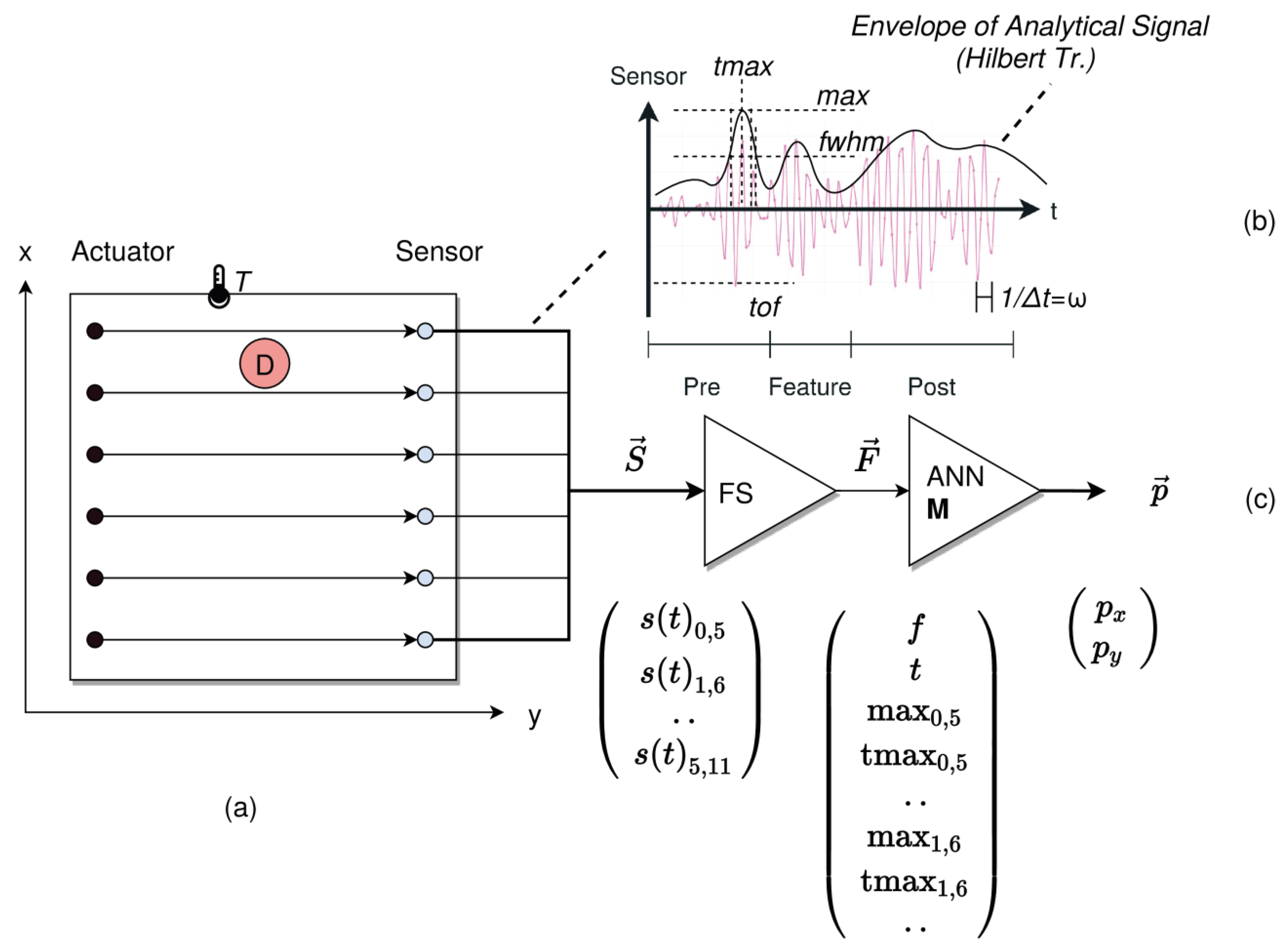
The data used in this work were time-resolved ultrasonic signal data from an active measuring technique, i.e., when the signal response is the result of an active stimulus. A piezo-electric actuator that is coupled to the surface of the device under test (or embedded inside a lamination layer, such as the CFL plate used in this work) injects a 5-cycle Hanning window wave burst. The guided waves propagate through the material and partially on the surface. The guided wave interacts with the material and potential defects and damage. The interaction strength of damage depends on the spatial actuator–sensor path (Figure 1a). A damage interaction leads to a change in the original damage-free signal only in a small part of the signal with respect of the time dimension, as shown in Figure 1b, which indicates the Region of Interest (ROI) for damage-related features, typically derived from the envelope of the wave signal. The identification of the ROI is difficult, depending on a priori knowledge and the strength of the damage–wave interaction, which can be weak. Beside using raw time series data, typically transformed in frequency or time–frequency space using fast Fourier transform (FFT) or discrete wavelet transforms (DWT), characteristic feature parameters should be derived numerically from the signal.

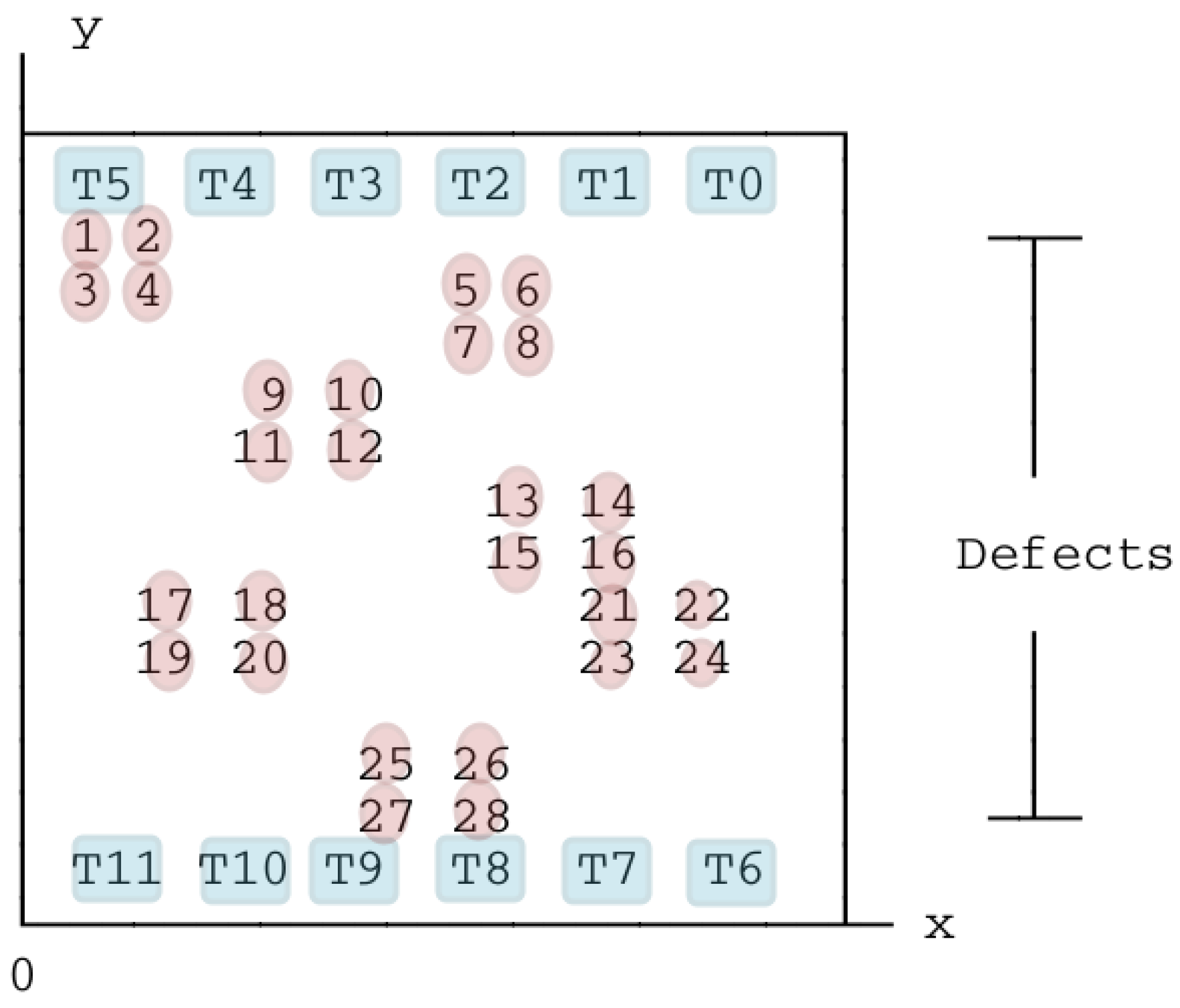
As shown in Figure 1a, there are multiple transducers that can be used as an actuator or sensor. Multiple paths can be measured simultaneously, creating the sensor signal vector S. A feature vector F is derived from S (explained in the next section). Finally, a damage position p is the output of a predictor function. The extrinsic parameter device temperature could be changed (by a temperature chamber). There are two dataset groups that are available from the OGW data base featuring different measurements with pseudo-defects (principle positions shown in Figure 2):

• Five data tables with GUW signals with a dynamic temperature profile (20–60 °C); a sub-set of four defect positions D4, D10, D14 and D24; and a baseline measurement without a defect (called dynamic dataset herein);
• Thirty-three data tables with GUW signals recorded at a static temperature (24 °C), all 28 defect positions and a baseline measurement (called static dataset herein).

3. Feature Selection

In general, the aim of feature selection is the mapping of the raw time-resolved signal data s(t) of a damaged area with a relevant and representative small set of feature parameters f^→ using a feature selection function ψ:

$$\begin{array}{l}{\psi }_{i,j}:{\overrightarrow{s}}_{i,j}\to {\overrightarrow{f}}_{i,J}\\ \overrightarrow{s}=\langle s\left(t=0\right),s\left(t=1\right),..\rangle \\ \overrightarrow{F}=\left(\begin{array}{c}T\\ \omega \\ {\overrightarrow{f}}_{i,j}\end{array}\right)\end{array}$$

(1)

The GUW depends on the temperature of the medium in which the waves propagate, and as a result the damage features are dependent on the environmental state, mostly the temperature [7]. Relevant damage features are contained in the envelope of the signal burst, commonly related to the envelope of the dominant wave group, mainly the height (max), the time point of the maximum (tmax) and the full width at half maximum (fwhm). These parameters strongly depend on the material’s temperature as a result of the wave propagation. Details can be found in [7]. To derive the envelope of the signal burst, two numerical approaches can be used:

• Computing the magnitude of the complex analytical signal through a Hilbert transformation of the time-resolved signal s(t) (non-iterative approach);
• By finding the maximum signal peak and performing a constrained Gaussian peak fitting of the wave group around the maximum—i.e., fitting a Gaussian function to the envelope of the signal group (iterative approach).

For a given time-dependent signal s(t), the analytical signal s_a(t) is given as:

$$\begin{array}{l}{s}_a\left(t\right)=s\left(t\right)+\mathrm{i}\left[s\left(t\right)\ast \frac{1}{\pi t}\right]=s\left(t\right)+\mathrm{i}\mathscr{H}\left\{s\left(t\right)\right\}\\ H\left(s\left(t\right)\right)=\left|s_a\left(t\right)\right|\end{array}$$

(2)

The analytical signal is based basically on a convolution operation (*), but it can be derived by using the discrete Fourier transforms (DFT, and fast version FFT):

$$\begin{array}{l}X\left[\omega \right]=\tau {\displaystyle \sum _{n=0}^{N-1}}s\left[n\right]e^{-\mathrm{i}2\pi \omega n\tau }\\ Z\left[m\right]=\{\begin{array}{cc}X\left[0\right]& \mathrm{if} m=0\\ 2X\left[m\right]& \mathrm{if} 1\le m\le \frac{N}{2}-1\\ X\left[\frac{N}{2}\right]& \mathrm{if} m=\frac{N}{2}\\ 0& \mathrm{if} \frac{N}{2}+1\le m\le N-1\end{array}\\ H\left[n\right]=\frac{1}{NT}{\displaystyle \sum _{m=0}^{N-1}}Z\left[m\right]e^{\mathrm{i}2\pi m\frac{n}{N}}\end{array}$$

(3)

τ: sampling interval; ω: frequency; X: forward discrete Fourier transform (DFT); Z: Hilbert transform in frequency domain; H: final Hilbert transform in time domain by using the inverse DFT.

Characteristic features f_i derived from the envelope of the signal s(t) are [7] (see also Figure 1b,c):

• The absolute (normalized) maximum value of the dominant envelope peak, max;
• The time position at the maximum, tmax;
• The full width at half maximum of the envelope peak, fwhm;
• A time-of-flight parameter, tof.

All these features are dependent on the signal frequency ω and the temperature T, and for the normalization on the stimulus amplitude—i.e., f_i = f_i(ω,T).

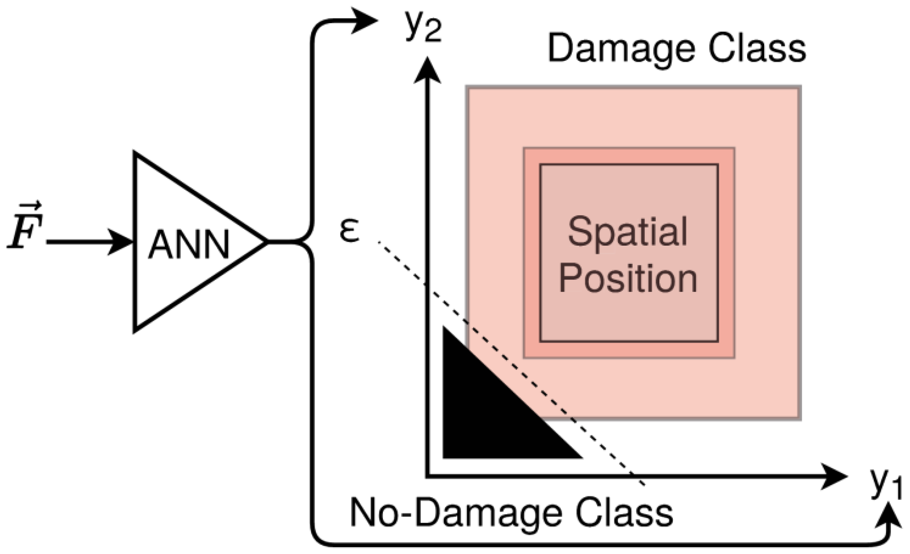
4. Predictor Model Function

A classical feed-forward fully-connected neuronal network with one or two hidden layers is used to predict the damage position p = (x, y) in normalized coordinates x = [0, 1], y = [0, 1] implemented with a modified version of the neataptic ANN software library [9]. An output |p| < ε indicates the absence of a damage, i.e., x and y ≈ 0. Therefore, the predictor function combines a classifier and a spatial regression model, shown in Figure 3, reducing computational and memory complexity, a constraint for implementation in embedded sensor node systems.

The input of the network is a vector containing the material temperature T, the signal frequency ω and selected features from all six straight path (φ = 0) ultrasonic signal measurements. Typical features derived from the feature selection process are max and tmax. Additional computed feature parameters are time of flight (tof) and the full width at half maximum (fwmh).

$$\begin{array}{l}M\left(F\right):\overrightarrow{F}\to \overrightarrow{p}\overrightarrow{F}=\left(\begin{array}{c}T\\ \omega \\ {\max }_{i,j}\\ {\mathrm{tmax}}_{i,j}\\ ..\end{array}\right),\forall \left(i,j\right)\in \mathrm{conf}\left(i,j\right)\\ \mathrm{conf}\left(i,j\right)=\left\{\langle 0,6\rangle ,\langle 1,7\rangle ,\langle 2,8\rangle ,\langle 3,9\rangle ,\langle 4,10\rangle ,\langle 5,11\rangle \right\}\\ \overrightarrow{p}=\left(x,y\right)\end{array}$$

(4)

The input layer consists of |F| neurons depending on the selected sub-set of features. The output layer consists of two neurons providing estimations of the damage’s x and y positions, respectively. The output is normalized to a spatial range of [0.2, 0.7] that corresponds to a geometric range of [0, 0.5 m]. The non-damaged case is predicted if |p| < ε (e.g., ε = 0.02). Any p_x or p_y ∈ (0.7, 1.0] or (ε, 0.2) indicates a prediction error!

5. Functional Scaling

The target host environment for the deployment of the damage predictor function is an embedded sensor node equipped with a low-resource and low-power microcontroller. This sensor node acquires the multi-path raw sensor signals, performs the feature selection pre-processing and applies the predictor function. Even if the training of the predictor function takes place offline, the application of the predictor function should be performed online. The predictor function consists of the signal pre-processing with the previously introduced feature selection algorithm, and the forward computation of the ANN.

Table 1. Computation times for the central feature selection (computation of analytical signal by Hilbert transform) and using the ANN predictor model on various processing platforms (gcc: C and native machine code; node.js/quickjs: JavaScript code).

Host	Platform	Function	Performance
Intel i5-3427U 1.80 GHz	node.js 8.12	dhrystone benchmark	5400 k dhry/s
Intel i5-3427U 1.80 GHz	node.js 8.12	ann-model-14-8-2	10 μs/pred
Intel i5-3427U 1.80 GHz	gcc 6.3 -O2	ann-model-14-8-2	0.8 μs/pred
Intel i5-3427U 1.80 GHz	node.js 8.12	hilbert-fft (4096 points)	1 ms/trans
Intel i5-3427U 1.80 GHz	gcc 6.3 -O2	hilbert-fft (4096 points)	0.5 ms/trans

and

Table 2. Computation times for the central feature selection (computation of analytical signal by Hilbert transform) and using the ANN predictor model on various processing platforms (gcc: C and native machine code; node.js/quickjs: JavaScript code).

Host	Platform	Function	Performance
Raspberry Pi Zero W 1.0 GHz	node.js 8.12	dhrystone benchmark	200 k dhry/s
Raspberry Pi Zero W 1.0 GHz	quickjs 2021.3	dhrystone benchmark	8 k dhry/s
Raspberry Pi Zero W 1.0 GHz	node.js 8.12	ann-model-14-8-2	30 μs/pred
Raspberry Pi Zero W 1.0 GHz	quickjs 2021.3	ann-model-14-8-2	300 μs/pred
Raspberry Pi Zero W 1.0 GHz	gcc 6.3 -O2	ann-model-14-8-2	5 μs/pred
Raspberry Pi Zero W 1.0 GHz	node.js 8.12	hilbert-fft (4096 points)	25 ms/trans
Raspberry Pi Zero W 1.0 GHz	quickjs 2021.3	hilbert-fft (4096 points)	300 ms/trans
Raspberry Pi Zero W 1.0 GHz	gcc 6.3 -O2	hilbert-fft (4096 points)	5 ms/trans

show typical computational times for the feature selection, mostly by Hilbert transformation and the ANN application. Different host computer architectures and processing platforms (i.e., native machine code and VMs like node.js and quickjs) were evaluated. For both algorithms there was a JavaScript and a C implementation. The Raspberry Pi Zero is a small, low-powered embedded computer. Although it is still oversized compared with material-integrated nano-computers (less than 100 MHz CPU clock and about 100 kB RAM), both algorithms can be implemented and processed on such low-resource systems.

The computational complexity of the ANN is negligible compared with the feature computation process (about 1:1000). For each prediction, m Hilbert transformations must be performed for m paths. However, even using the slowest (but embeddable) platform, JavaScript quickjs, the entire prediction required less than two seconds on a RP Zero. Assuming a computational power ratio of 1:100 for the RP Zero compared to a material-integrated nano computer (e.g., the ancient Micro Mote M3), a native code implementation of the full predictor program will require only three seconds of computation, which can be still considered sufficiently fast. Probably, finite and infinite response (FIR/IIR) filter-bank approaches approximating the Hilbert transform can provide additional reductions of the computational complexity.

6. Evaluation

The GUW signal data [10,11] were taken from the OGW server, and several signal datasets were stored in SQL tables for further processing. The feature selection computations using the Hilbert transform and conventional peak analysis algorithms were originally performed with Python code [7]. The predictor function was implemented with a modified version of the Neataptic JavaScript ANN framework [9]. The experimental matrix consisted of:

• Two datasets: (D) dynamic temperature profile (T = 20–50 °C, 4 defect positions) and (S) static temperature (T = 24 °C, 28 defect positions) datasets—GUW sensor data of a 500 × 500 mm CFK plate with attached pseudo-defects;
• Different feature parameter sets: {max, tmax, T}, {max, tmax, fwhm, T}, {max, tmax, fwhm, tof, T}.
• Different network architecture configurations: [I, H₁, H₂,..., O].
• Two different input variable scaling methods: Static, i.e., a feature is scaled equally for all paths with a fixed scale; Auto: a feature is scaled automatically and independently for all paths.
• Different training and test set combinations: {D/D, D/S, SD/SD, SD/Dm SD/S}.

Due to the limited dataset variance, the model accuracy was tested with training data with different combinations of the dynamic and static temperature datasets. Although a Monte Carlo simulation was used to augment training data by adding Gaussian noise, no further data augmentation was performed. Therefore, the results shown in

Table 3. Prediction results for ω = 40 kHz (D: dynamic temperature dataset, S: static temperature).

Features F→ (40 kHz)	Model [Layer]	Scaling	Training Data [%]	Test Data [%]	Mean. Pos. Error [%]	Position Incorrect [%]	TP/FP, TN/FN [%]
max, tmax, T	[14, 8, 2]	Fixed	D = 100, S = 100	D = 100, S = 100	3	4	100/0, 100/0
max, tmax, T	[14, 8, 3, 2]	Fixed	D = 100, S = 100	D = 100, S = 100	5	9	100/0, 100/0
max, tmax, T	[14, 8, 3, 2]	Auto	D = 100, S = 0	D = 100, S = 0	2	0	100/0, 100/0
max, tmax, fwhm, T	[20, 8, 2]	Fixed	D = 100, S = 100	D = 100, S = 100	9	16	100/0, 91/9
max, tmax, fwhm, T, tof	[26, 8, 2]	Fixed	D = 100, S = 100	D100, S = 100	6	21	100/0, 100/0
max, tmax, T	[14, 8, 3, 2]	Fixed	D = 100, S = 0	1D = 100, S = 0 2D = 0, S = 100	13 248	10 270	1100/0, 100/0 220/80, 100/0

and

Table 4. Prediction results for ω = 80 kHz (D: dynamic temperature dataset, S: static temperature).

Features F→ (80 kHz)	Model [Layer]	Scaling	Training Data [%]	Test Data [%]	Mean. Pos. Error [%]	Position Incorrect [%]	TP/FP, TN/FN [%]
max, tmax, T	[14, 8, 2]	Fixed	D = 100, S = 100	D = 100, S = 100	20	50	100/0, 33/67
max, tmax, T	[14, 8, 4, 2]	Fixed	D = 0, S = 100	D = 0, S = 100	16	36	100/0, 0/100
max, tmax, T	[14, 8, 3, 2]	Auto	D = 100, S = 0	D = 100, S = 0	4	3	100/0, 100/0
max, tmax, T	[14, 8, 3, 2]	Auto	D = 100, S = 100	D = 100, S = 100	12	27	100/0, 80/20
max, tmax, T	[14, 8, 3, 2]	Auto	D = 100, S = 0	1D = 100, S = 0 2D = 0, S = 100	15 260	13 285	1100/0, 100/0 20/100, 100/0

cannot conclude on the generalizability of the trained model. The position error threshold was set to 100 mm (error above was classified as an incorrect position prediction). The non-damage detection threshold was set to 0.05/1.0. The results in Table 3 and Table 4 show the average defect position estimation accuracy delivered by the predictor function; the fraction of incorrectly located defects (position error too large); and the binary defect classification rates—true positive (TP, damage) and true negative (TN, no damage) with their negative counterparts false positive (FP) and false negative (FN).

We observed:

• High accuracy of defect classification (100% TP, 100% TN), even under temperature variations in the range 20–50 °C, can be achieved by a network with only one hidden layer (eight neurons) and by using the major features max and tmax;
• The minor features, fwhm and tof, can be discarded, as they provided no benefit (in contrast, including them degraded model accuracy until the training dampened them);
• Reasonable defect localisation with an average position error below 20 mm is possible;
• High sensitivity of prediction results to feature parameter noise (even if low as 5% Gaussian noise) and feature variable scaling (static and fixed verses dynamic and automatic);
• The training process and prediction accuracy showed high sensitivity to data normalization (scaling);
• Probably only a specialized model was trained (due to low variances in defect positions and variations of environmental parameters);
• Suitable learning rates were between 0.05 and 0.2;
• A model trained by the dynamic dataset (only four defects) showed low accuracy for the prediction of the static dataset (even concerning the four damage areas contained in the static dataset too);
• The accuracy of the prediction model depended on the signal frequency (40 kHz outperformed 80 kHz);
• One hidden layer was typically suitable for achieving high accuracy, showing a low non-linearity degree of this problem;
• The training time for one model was a few minutes on a generic desktop computer (JavaScript processed by node.js or in the WEB browser).

7. Conclusions

Using multi-path sensing of guided ultrasonic waves, advanced feature selection and a simple artificial neural network, we were able to detect pseudo-defects applied to a CFL plate with a high probability (typically nearly 100%) and high position accuracy (typically below 20 mm or better) with a wide range of material temperatures (20–50 °C). The advanced feature selection is based on a Hilbert transform of the time-resolved signal data and maximum peak analysis. The computed features are the input vectors for the ANN predictor function, which combines a binary damage/defect classifier with a two-dimensional position regression of the damage. Typically, only one hidden layer with a few neurons was suitable for achieving high accuracy and a high TP/TN rate.

It was shown that the proposed analysis method is suitable for implementation in embedded systems, including material-integrated nano-computers, where it could provide damage detection within 10 s after signal measurement, which is sufficient for a broad range of applications in SHM. Using signal down-sampling and optimized implementations of the FFT and Hilbert transform should provide prediction times below 1 s (on an embedded nano-computer) The feature selection reduces the input data vector’s dimensions from 4096 samples × 6 paths (24,576) to a minimum number of 14 (maximal 26 depending on the selected feature sub-set)!

This work was based on already extant data lacking variance with respect to defect positions, material properties and environmental conditions. Further investigations using GUW measurements for a fibre metal laminate plate are undergoing and should create suitable training and test datasets that will allow assessment of the robustness and generalization degree of the trained model.

References

- Moll, J.; Kexel, C.; Pötzsch, S.; Rennoch, M.; Herrmann, A.S. Temperature affected guided wave propagation in a composite plate complementing the open guided waves platform. Nature 2019, 6, 191. [Google Scholar] [CrossRef] [PubMed]
- Teimouri, H.; Milani, A.S.; Seethaler, R.; Heidarzadeh, A. On the impact of manufacturing uncertainty in structural health monitoring of composite structures: A signal to noise weighted neural network process. Open J. Compos. Mater. 2016, 6, 28–39. [Google Scholar] [CrossRef] [Green Version]
- Roseiro, L.; Ramos, U.; Leal, R. Neural networks in damage detection of composite laminated plates. In Proceedings of the 6th WSEAS International Conference on Neural Networks, Lisbon, Portugal, 16–18 June 2005; Volume 2005, pp. 115–119. [Google Scholar]
- Sarkar, S.; Reddy, K.K.; Giering, M.; Gurvich, M.R. Deep learning for structural health monitoring: A damage characterization application. In Proceedings of the Annual Conference of the Prognostics and Health Management Society, Denver, CO, USA, 3–6 October 2016; pp. 176–182. [Google Scholar]
- Bosse, S.; Lehmhus, D. Robust detection of hidden material damages using low-cost external sensors and machine learning. In Proceedings of the 6th International Electronic Conference on Sensors and Applications (ECSA), Online. 15–30 November 2019. [Google Scholar]
- Bosse, S. Learning damage event discriminator functions with distributed multi-instance RNN/LSTM machine learning—Mastering the challenge. In Proceedings of the 5th International Conference on System-Integrated Intelligence Conference, Bremen, Germany, 11–13 November 2020. [Google Scholar]
- Polle, C.; Koerdt, M.; Maack, B.; Focke, O.; Herrmann, A.S. Introduction of the temperature scaling method for structural health monitoring with guided ultrasonic waves. Structural Health Monitoring. Sage, 2022; submitted. [Google Scholar]
- Wang, Y.-S.; Gao, L.; Yuan, S.; Qiu, L.; Qing, X. An adaptive filter-based temperature compensation technique for structural health monitoring. J. Intell. Mater. Syst. Struct. 2014, 25, 2187–2198. [Google Scholar] [CrossRef]
- Wagenaar, T. Available online: https://wagenaartje.github.io/neataptic (accessed on 1 January 2020).
- Open Guided Waves Data Base. Available online: http://openguidedwaves.de/downloads (accessed on 1 January 2020).
- Moll, J.; Kexel, C.; Kathol, J.; Fritzen, C.-P.; Moix-Bonet, M.; Willberg, C.; Rennoch, M.; Koerdt, M.; Herrmann, A. Guided waves for damage detection in complex composite structures: The influence of omega stringer and different reference damage size. Appl. Sci. 2020, 10, 3068. [Google Scholar] [CrossRef]