
Determinants of the European Sovereign Debt Crisis: Application of Logit, Panel Markov Regime Switching Model and Self Organizing Maps

1
CNRS, GREDEG, Bâtiment 2, Campus Azur du CNRS, Université Côte d’Azur, 250 rue Albert Einstein, CS 10269, F-06905 Sophia Antipolis Cedex, France
2
Department of Economics, Kirklareli University, Kayali Kampüsü B-Blok, 39000 Kirklareli, Turkey
*
Author to whom correspondence should be addressed.
Entropy 2023, 25(7), 1032; https://doi.org/10.3390/e25071032
Submission received: 5 June 2023
/
Revised: 1 July 2023
/
Accepted: 5 July 2023
/
Published: 8 July 2023
(This article belongs to the Special Issue Applications of Statistical Physics in Finance and Economics)
Abstract
:The study aims to empirically identify the determinants of the debt crisis that occurred within the framework of 15 core EU member countries (EU-15). Contrary to previous empirical studies that tend to use event-based crisis indicators, our study develops a continuous fiscal stress index to identify the debt crises in the EU-15 and employs three different estimation techniques, namely self-organizing map, multivariate logit and panel Markov regime switching models. Our estimation results show first that the study correctly identifies the time and the length of the debt crisis in each EU-15-member country. Empirical results then indicate, via three different models, that the debt crisis in the EU-15 is the consequence of deterioration of both financial and macroeconomic variables such as nonperforming loans over total loans, GDP growth, unemployment rates, primary balance over GDP, and cyclically adjusted balance over GDP. Furthermore, variables measuring governance quality, such as voice and accountability, regulatory quality, and government effectiveness, also play a significant role in the emergence and the duration of the debt crisis in the EU-15.
1. Introduction
Over the last decade, the European Union went through the most severe economic and political crisis since its creation following World War II. Some economists (i.e., [1,2,3,4,5,6,7]) stated that the crisis was the result of contagion of the US subprime crisis to Europe: as the crisis spread to Europe, governments and central banks heavily intervened in real and financial sectors to limit the negative impacts of the crisis. These expansionary policies and bank rescue plans (in other words, nationalization of private debt) resulted in a dramatic rise in public debt stock, leading then to a sovereign debt crisis in some Eurozone member countries.
Some argued that the crisis was related to increasing fiscal deficits and rising public debt stock, but these problems are the consequences of the structural factors associated with the Eurozone (i.e., [8,9,10,11,12,13,14]). The main argument here is the Eurozone is not an optimum currency area a la Mundell [15], since there is no risk sharing system such as an automatic fiscal transfer mechanism to redistribute money to areas/sectors which have been adversely affected by the capital and labor mobility. Moreover, Eurozone is a monetary union without a fiscal union: this design, permitting the free riding of fiscal policies within a framework of common monetary policy, led to differences in inflation rates within the Eurozone member countries. Inflation differences in turn caused a decrease in the trade competitiveness of high-inflation countries, i.e., Greece, Spain. As the option of improving the competitiveness of the economy through exchange rate depreciation was not available, because of the common currency, trade deficits steadily rose in the Southern peripheral countries, leading to constant increases in public debt stock [16]. This was not an important problem until the outbreak of the global financial crisis. With the transition to European Monetary Union (EMU), increasing capital inflows towards peripheral countries resulted in low interest rates facilitating the rollover of the debt stock. In addition, low interest rates led to a decrease in household savings and increased consumption, causing external deficits and an increase in private debt stock.
This study aims to empirically identify the determinants of the European debt crisis. To do so, we employ three different estimation techniques, namely SOM, logit, and Markov models. The main reason to use different methods is the fact that using different methodologies have led to inconsistent results in terms of crisis determinants and crisis prediction (see [17,18,19,20] for further discussion). Hence, we first apply the SOM approach, which allows us to visualize, via crisis maps created for each country, the transition from noncrisis to crisis states. Furthermore, the SOM analysis gives us variables’ order of importance in explaining the occurrence of the debt crises in the EU member countries. In other words, the SOM analysis serves as a filter to determine which indicators should be included into the logit and Markov model estimations. Then, we estimate logit and Markov models with the variables found to be significant by the SOM approach.
This paper brings empirical contributions to the literature on fiscal stress in a monetary union [21,22,23,24]. In the first step, we identify and date debt crises by defining a new fiscal stress index. Second, we use a large data set composed of 51 leading indicators to explain the European debt crises. In particular, this paper includes an important number of governance indicators that have largely been ignored in explaining debt crises. Third, we use different econometric tools—namely the self-organizing maps (SOM), the multivariate logit model (MLM), and the panel Markov regime switching model (PMRSM)—to identify the determinants of the European debt crisis. Our study therefore offers the opportunity of a comparative analysis between different model estimations, which has not been conducted yet in the literature.
According to the results, in addition to financial and macroeconomic variables, such as nonperforming loans over total loans, GDP growth, primary balance over GDP, unemployment, and cyclically adjusted balance over GDP, governance variables (i.e., voice and accountability, regulatory quality and government effectiveness) also play a significant role in the emergence of the European debt crisis. In addition, forecast performances estimates suggest that our different models perform relatively well to predict the debt crisis in the Eurozone.
2. Data and Methodology
2.1. The Definition of Fiscal Stress Index
Debt crises are usually identified and dated by a combination of events, such as the inability of borrowers to pay the interest or principal on time, large arrears, or large IMF loans to help the borrower avoid a default. In other words, dating debt crises is generally event-based and is typically founded on the available ex post figures (i.e., [21,25,26]). However, this dating method has several shortcomings. It is based primarily on information about government actions undertaken in response to fiscal stress and depend on information obtained from regulators and international organizations or rating agencies. In addition, the events method identifies crises only when they are severe enough to trigger market events; crises successfully contained by prompt corrective policies are neglected. This means that empirical work suffers from a selection bias. Therefore, in order to fulfill these shortcomings, we develop a fiscal stress index like currency crisis indictors, a la Eichengreen et al. [27] or Kaminsky and Reinhart [28], in order to identify the dates of debt crisis episodes occurred in EU-15 countries over the period from 2003–2015.
The data used for constructing the fiscal stress index (FSI) are gathered from Oxford Economics and IMF International Financial Statistics for the period from 2003–2015. Our fiscal stress index is defined as a continuous variable rather than event-based, contrary to previous studies. The bond yield pressure, imputed interest rate on general government debt minus the real GDP growth rate, public sector borrowing requirements, general government gross debt, and cyclically adjusted primary balance variables are used in calculating our fiscal stress index. The selection of variables in the construction of the index is based on Baldacci et al. [21], McHugh et al. [26], and Hernandez de Cos et al. [23]. Note also that the variables are standardized or weighted according to the empirical crisis literature. The weights of the components of the crisis index are chosen to equalize their volatility and thus avoid the possibility of one of the components dominating the index, allowing us to obtain consistent results concerning dates of debt crises.
The fiscal stress index is calculated as follows:
where BYP (bond yield pressure) is government bond spreads (relative to 10-year US Treasury bonds), r − g is the imputed interest rate on general government debt minus real GDP growth rate, GGGD is general government gross debt, and CAPB indicates cyclically adjusted primary balance/GDP. Sub-indexes represent t as time, i as country, and is the differential operator. Increases in BYP, r − g, PSBR, and GGDD augment fiscal pressure, while increases in CAPB reduce fiscal pressure. Because increases in CAPB indicate a balanced budget, its effect is expected to be negative.
We define a debt crisis hitting country i at time t, Ci,t, as a binary variable that can assume either 1 (when the FSI is above its threshold value) or 0 (otherwise):
A critical point is to choose an ‘optimal’ threshold value. Several papers determine an arbitrary threshold. The higher the threshold level is, the lower the number of detected crises is, and vice versa. Therefore, this arbitrary threshold method results in different numbers and effective dates of crises as empirically shown by Kamin et al. [29], Edison [30], and Lestano and Jacobs [31] in the case of currency crises.
In order to avoid problems related to threshold level, we consider different methods based on Candelon et al. [32] to determine the optimal threshold value for the fiscal stress index of each EU-15 country. For this purpose, we use accuracy measures, sensitivity-specificity graphics, and the KLR cut-off method Kaminsky et al. [33] to select the optimal threshold. In this study, we present two different cut-off values, country-specific and global, in the KLR cut-off method. The country-specific cut-off value is the cut-off value determined according to the country’s own fiscal stress index, while the global cut-off value is the cut-off value obtained from the fiscal stress index of all EU-15 countries.
The fiscal stress index for each EU-15 country is constructed according to the Equation (1). In order to identify debt crisis periods, we need to determine optimal threshold (cut-off) values, which are calculated using three different methods (see Table 1). Bold numbers indicate the optimal cut-off values for each country.
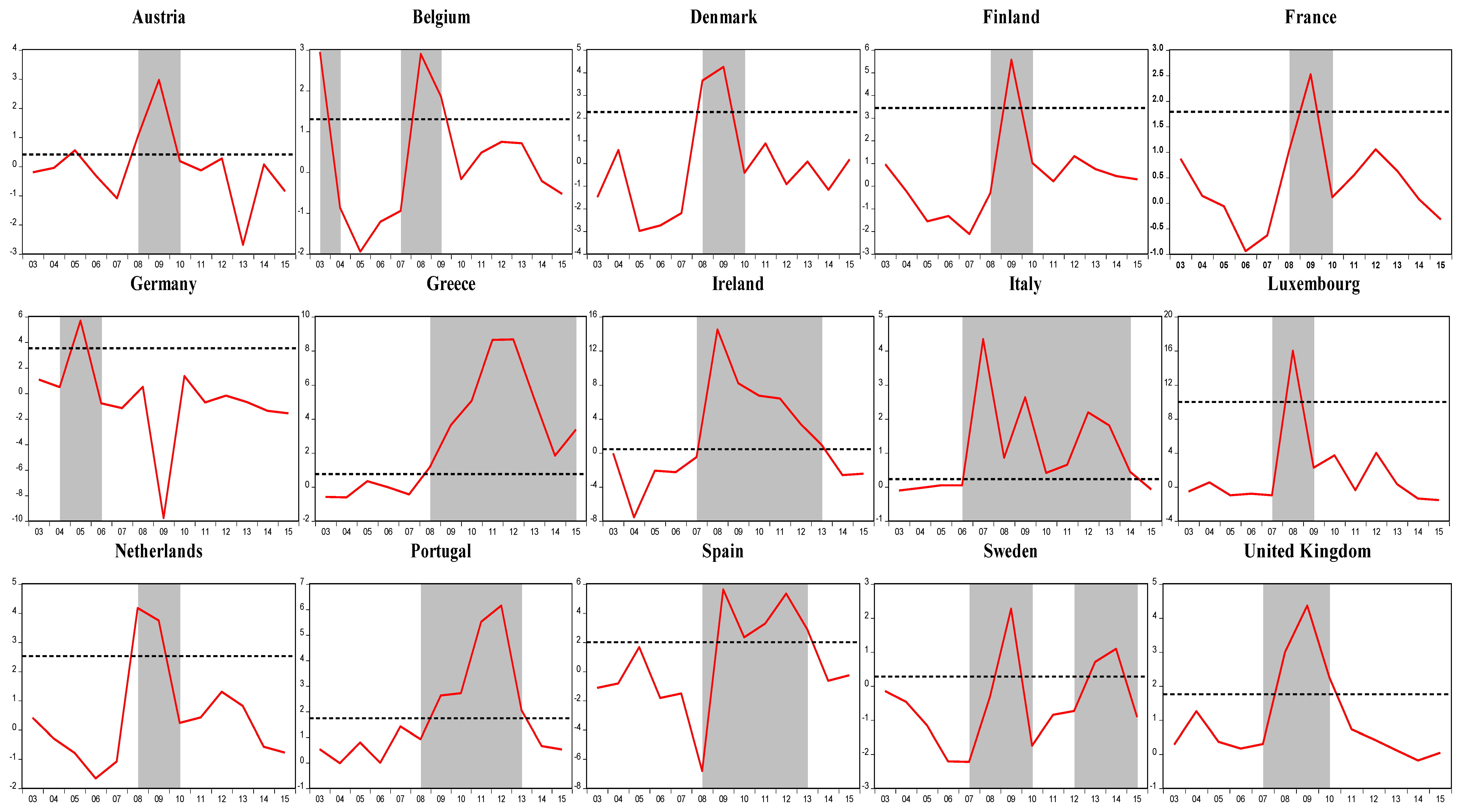
Figure 1 presents the crisis and noncrisis periods for EU-15 countries: shaded zones indicate crisis periods, in other words, the period where the index value exceeds the optimal threshold value. As clearly seen from Figure 1, all EU-15 countries except for Germany seem to have gone through the debt crisis following the global financial crisis. As expected, the debt crisis in Greece, Ireland, Spain, the United Kingdom, Italy, and Portugal seem to have lasted longer compared to other countries. In addition, Greece seems to have not fully recovered from the debt crisis by the end of 2015.
When we compare our results with those of previous literature [21,22,23], we observe that they do not find any crisis episode in the cases of Austria, Belgium, Finland, France, and the Netherlands in the post-2003 period (see Table 2). Our fiscal stress index identifies more ‘debt crisis’ episodes than previous empirical studies applied to debt crises, since it measures the pressure or stress level in a country contrary to other fiscal stress definitions that focus mainly on default events. On the contrary, our results show that Austria in 2009, Belgium in 2003, 2008, and 2009, Finland in 2009, France in 2009, and the Netherlands in 2008 and 2009 had severe fiscal problems. Furthermore, Hernandez de Cos et al. [23] state that Greece, Ireland, Italy, and Portugal had a debt crisis from 2008 to 2010, while our index indicates that Greece from 2008 to 2015, Ireland from 2008 to 2013, Italy from 2007 to 2014, and Portugal from 2009 to 2013 suffered a debt crisis.
2.2. Leading Indicators
Our dataset consists of 51 leading indicators. The selection of leading indicators is based on the studies by Manasse et al. [34], Baldacci et al. [21], McHugh et al. [26], Berti et al. [22], and Hernandez de Cos et al. [23]. Table 3 presents definitions, sources, and descriptive statistics for the selected leading indicators used in the study. We consider five sets of indicators. The first set consists of public and real sector variables: GDP, inflation, unemployment, government expenditure/GDP, primary balance/GDP, cyclically adjusted balance/GDP, revenue/GDP, interest payments/revenue, interest payments/expenses, cash surplus/GDP, REER, savings/expenditures, tax revenue/GDP, and wages. The second category includes financial indicators that exert an influence on sovereign debt situations: bank capital/asset, nonperforming loans/total loans, banking sector leverage, M2/GDP, and banking crisis index. The study uses Laeven and Valencia’s [35,36] definition of a banking crisis.
Our third set of indicators encompasses different debt ratios: external debt/export, external debt/GDP, external debt government/GDP, external debt private/GDP, net debt/GDP, and household debt/GDP. Social indicators constitute our fourth set: health expenditure/GDP, public health expenditure/GDP, Gini coefficient, gross enrollment ratio, fertility rate, and age dependency ratio. Excessive increases in health expenditures, a deterioration in income distribution, a decline in education level and in fertility rate, and an increase in age dependency ratio are expected to increase the likelihood of a debt crisis.
Finally, our fifth and last set includes governance indicators. Only a very small number of studies have examined the effect of governance quality on the likelihood of debt crises [34,37]. In our study, unlike these studies, we directly use a large number of governance indicators in our model, including political stability risk rating, credit rating, trade-credit risk rating, government effectiveness, political stability and freedom from violence/terrorism, regulatory quality, rule of law, and voice and accountability variables. The deterioration of countries’ governance indicators is expected to increase the likelihood of a debt crisis. We use Kaufmann et al. [38] for defining governance indicators. Accordingly, voice and accountability cover freedom of expression, freedom of association, election of government, and free media for a nation’s citizens. Political stability and the freedom from violence/terrorism demonstrate the possibility of government destabilization or overthrow through unconstitutional political violence or terrorism. The government effectiveness indicator is the government’s policymaking and implementation quality and the credibility of its commitment to such policies, as well as the degree to which public services are independent of political repression. Rule of law shows the implementation of contracts in addition to opportunities for crime and violence; the quality of the police, courts, and property rights; and the level of trust and compliance of individuals with society. Control of corruption refers to the use of public power for special gains, with small or large corruption in addition to elite and private interests seizing public power. Political stability refers to the stability of the current government and the entire political system. Trade-credit risk rating means that the trading partner cannot fulfill its obligations. The democracy index refers to the country’s level of democracy.
2.3. Methodology
The previous literature testing the likelihood of a debt crisis rests on models such as logit-probit, signal approach, and Markov regime switching. We take a different approach by using three different methods in a comparative perspective. SOM or Kohonen maps (SOM model is a learning methodology introduced in the artificial neural network literature by Kohonen [39]), multivariate logit model (MLM), and panel Markov regime switching model (PMRSM). In addition, we test the stability of estimates. Last but not least, the predicting performance of each method is presented.
The SOM is a nonlinear and nonparametric method used to analyze high-dimensional datasets. Specifically, this model portrays low-dimensional images of high-dimensional data. An important contribution of this method compared to many econometric tools is that it does not rely on rigid assumptions. For instance, including too many variables at the same time may induce multicollinearity, where too many parameters cannot be predicted due to observation constraints. Although the SOM method has been used extensively in a large number of scientific fields since it first appeared in the literature, its use in economics is very rare (See [40,41,42,43,44,45,46,47,48,49]). For crisis literature, see Sarlin [50,51] and Sarlin and Marghescu [52].
A drawback of the SOM method is to interpret its components without specifying any definite relationship. In order to deal with this drawback, different approaches allow the identification of the significance of variables in SOM analysis. These approaches, which originate from the natural sciences, estimate different indexes such as the structuring index (SI), the relative importance index (RI), the cluster description index (CD), and the Spearman rank correlation index (SRC) [53].
The SI index has been originally developed by Park et al. [54] and Tison et al. [55,56]. A variable with a low SI value indicates that its effect on the cluster of the SOM map is low. In contrast, variables with high SI values explain a significant portion of the differentiation between cluster groups. The SI value of variable i is calculated as follows:
where the nominator and denominator show the weight and topological differences between j and k map units, respectively, while S represents the total number of map units.
In RI indexes, each variable is expressed based on the distance matrix as a pie chart proportional to the sum of the variables. In addition, the sum of these effects is standardized at 100. In other words, the importance of the variables in the model depends on the size they have in the pie chart. Accordingly, i is expected to have a high RI value if it is to have a high effect on the SOM structure.
Vesanto [57] uses the CD index, which expresses the variation in each cluster. Thanks to the CD index, the internal properties of each cluster can be displayed. The CD index is calculated as follows:
where σli and σi indicate the standard deviations of the variable in cluster l and the whole data set, respectively, while C shows the total number of clusters. A high CD value calculated for a variable means that the variable has high significance when it occurs in different clusters.
These methods can give quite a different order of importance in estimates. Hence, in order to deal with this potential inconsistency, not only do we estimate the previous indexes, but we also estimate two different overall indexes to avoid any contradictory results. The overall index (1) is calculated with the following steps. First, four different index values are converted into percentage values. For this, the highest value of each index is accepted as 100 and all other values are calculated based on this value. The main purpose of doing this is to provide a chance to compare different indexes from the same unit. Second, as each index is expressed as a percentage, the following calculation is made so that each index has an overall weight equal to:
where Xi represents the SI, RI, CD and SRC values of the variable i.
The overall index (2) is calculated as follows:
where , , , and show the standard deviations for the SI, RI, CD, and SRC indexes, respectively. , , , and indicate the means of the SI, RI, CD, and SRC indexes, respectively. In the overall index (2), we subtract the value of each index by its means and then divide the result by its standard deviation in order to standardize the indices and ensure that no factor dominates the overall index. The influence of extreme results is minimized with the aim of obtaining more consistent results. In addition, the consistency of the indexes was checked via factor analysis and the results were found to be consistent.
Logit-probit models are widely used in debt crisis literature (e.g., [25,34,58,59]). In such models, the dependent variable, i.e., the fiscal stress index, is converted into a binary variable. It has a value of “1” for values above the threshold (signaling debt crisis periods) and “0” otherwise (normal periods).
The Markov model is also frequently used in papers on financial crises (i.e., [32,60,61,62,63]). The Markov model uses the crisis index in a continuous format. As a result, unlike the logit model, no information is lost regarding crisis duration. Specifically, the Markov model does not require a prior dating of crises; instead, identifying crisis periods are determined within the model itself [64]. In our estimation results, the Davies test also indicates the number of regimes chosen to be appropriate for the predicted models. As in the case of Abiad [64], Alvarez-Plata and Schrooten [62], and Lopes and Nunes [65], who used the Markov model for crises, our study also assumes two different regime periods. The period with lower mean and volatility indicates the tranquil or no crisis regime, while the second regime with higher mean and volatility is said to be crisis.
3. Estimation Results
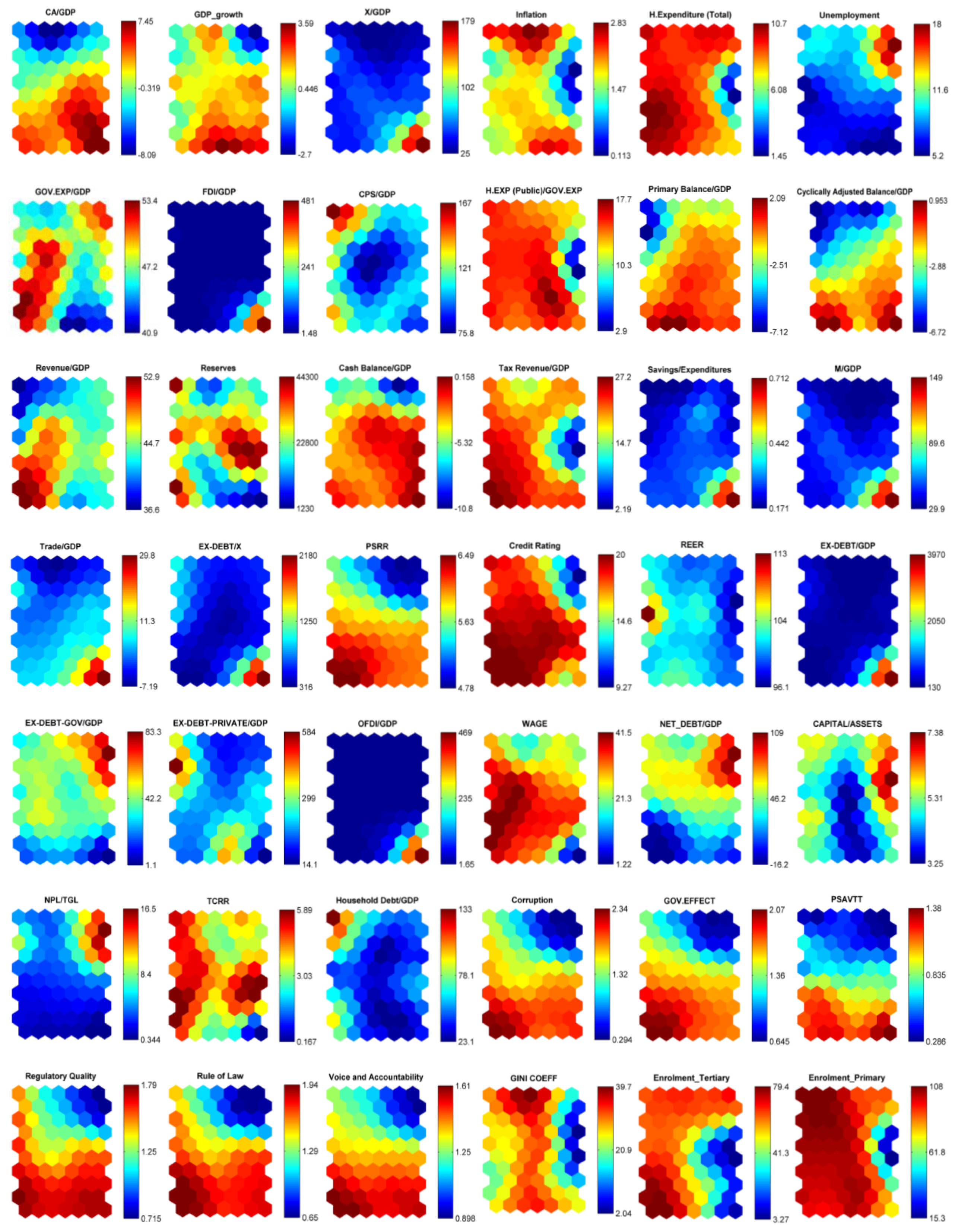
We employ three different estimation techniques, namely SOM, logit, and Markov models. Unlike other econometric approaches, the SOM approach allows the researcher to work with large datasets and has the ability to visually monitor, via crisis maps created for each country for the period 2003–2015, the transition from no crisis (tranquil) to crisis states. Furthermore, through the SOM analysis, we are able to determine the variables’ order of importance in explaining the occurrence of the debt crises in the EU member countries. In other words, the SOM analysis serves as a filter to determine which indicators should be included in the logit and Markov model estimations. Figure 2 exhibits our results for a large number of 51 indicators using the SOM estimation method. As seen in Figure 2, each variable has its own component matrix with two-dimensional visuality. Temperature maps allow us to determine the value that each variable takes in crisis and noncrisis periods, obtained from the Davies–Bouldin index. The scale on the right-hand side of each graph (component matrix) increases the readability. To be more precise, each graph in Figure 2 represents the values for the different neurons of the respective variable using a color code ranging from dark blue (low values) to dark red (high values). Before interpreting the results of the SOM analysis, some aspects of the analysis require clarification. First, all countries (input) are placed in only one specific neuron (output) [66]. Since the time dimension of countries is also used in our analysis, the neuron in which the country is placed may change over the years. The analysis results show that countries with similar indicators are placed in the same or close neurons, while countries with different characteristics are placed in more distant neurons. When making interpretations, it is important to note that regardless of the variable analyzed, the location of the country is the same place, i.e., the same neuron. For example, the location of the neuron where Austria is located in 2015 is the same in the component matrix of all variables. Therefore, the value in the component matrix of that variable is interpreted according to the scale on the right side. Figure 2 shows the clusters of countries in the lower right corner. The weight vectors of the SOM neurons reveal the effect of each variable in determining the characteristics of the clusters [67]. The figure shows that there are two different clusters. The first cluster is the crisis cluster shown in yellow. The second cluster is the no crisis cluster shown in red.
Figure 2 shows that the likelihood of the debt crisis jumps with an increase in inflation, unemployment rate, budget deficit-to-GDP ratio, public and private external debt as the share of GDP, household debt, nonperforming loans, age dependency ratio, bank leverage, M2 over GDP, banking crisis index, and interest payments. Figure 2 also suggests that countries in debt crisis have low growth rates, low export-to-GDP ratio, low reserves, low shares of public revenues and taxes to GDP, and low credit ratings. Figure 2 shows the impact of governance indicators on the outbreak of the European debt crisis: estimates indicate that high income inequality, high corruption, low government effectiveness, low political stability risk-rating, low political stability (PSVATT), low regulatory quality, low rule of law, and low voice and accountability increase the crisis probability. FDI over GDP, the ratio of health expenditures to public expenditures, total health expenditures, savings/expenditures, the ratio of imports to GDP, the ratio of foreign trade balance to GDP, OFDI over GDP, capital over asset, and TCRR do not seem to have an effect on the occurrence of the European debt crisis. Finally, indicators related to education do not seem to have an impact on debt crises. It is worth highlighting that our SOM results are consistent with economic intuitions. The results of the SOM analysis are quite similar to the literature. Previous studies in the literature have found that increases in short-term debt, total external debt to GDP ratio, current account deficit to GDP ratio, inflation, level of reserves/GDP ratio, political problems, and trade openness increase the probability of debt crisis. They also find that decreases in foreign exchange reserves, real GDP growth, and primary and overall fiscal balance to GDP ratios are important determinants of debt crises [22,23,25,34,58,59,68,69].
In order to identify the unobserved relationships of the component matrixes, Table 4 exhibits the mean and standard deviation of each leading indicator in crisis and no crisis periods. Overall, results from the SOM analysis are consistent with the results presented in Table 4. For instance, the growth rates of countries in crisis zone tend to be low, leading to a decrease in these countries’ tax revenues and to a rise in both social transfers and unemployment benefits.
Table 5 and Table 6 present the ranking of 51 explanatory variables according to the six indexes selected in our study. In particular, results from the two overall indexes (Table 6) show that the ratio of nonperforming loans over total loans, primary balance over GDP, public sector borrowing requirement, corruption, cash balance over GDP, unemployment, voice and accountability, regulatory quality, rule of law, GDP growth, government effectiveness, and cyclically adjusted balance over GDP are the 10 most important indicators in explaining the outbreak of the European debt crisis. These 10 variables will be used in both logit and Markov estimation.
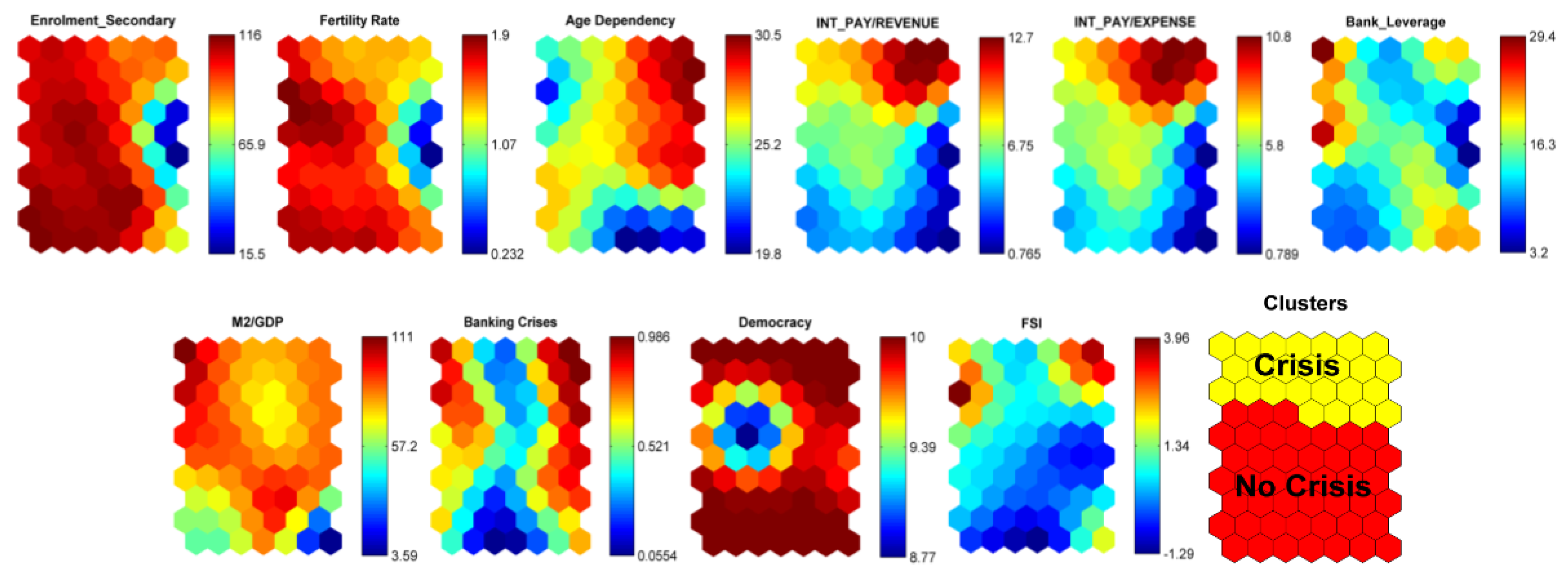
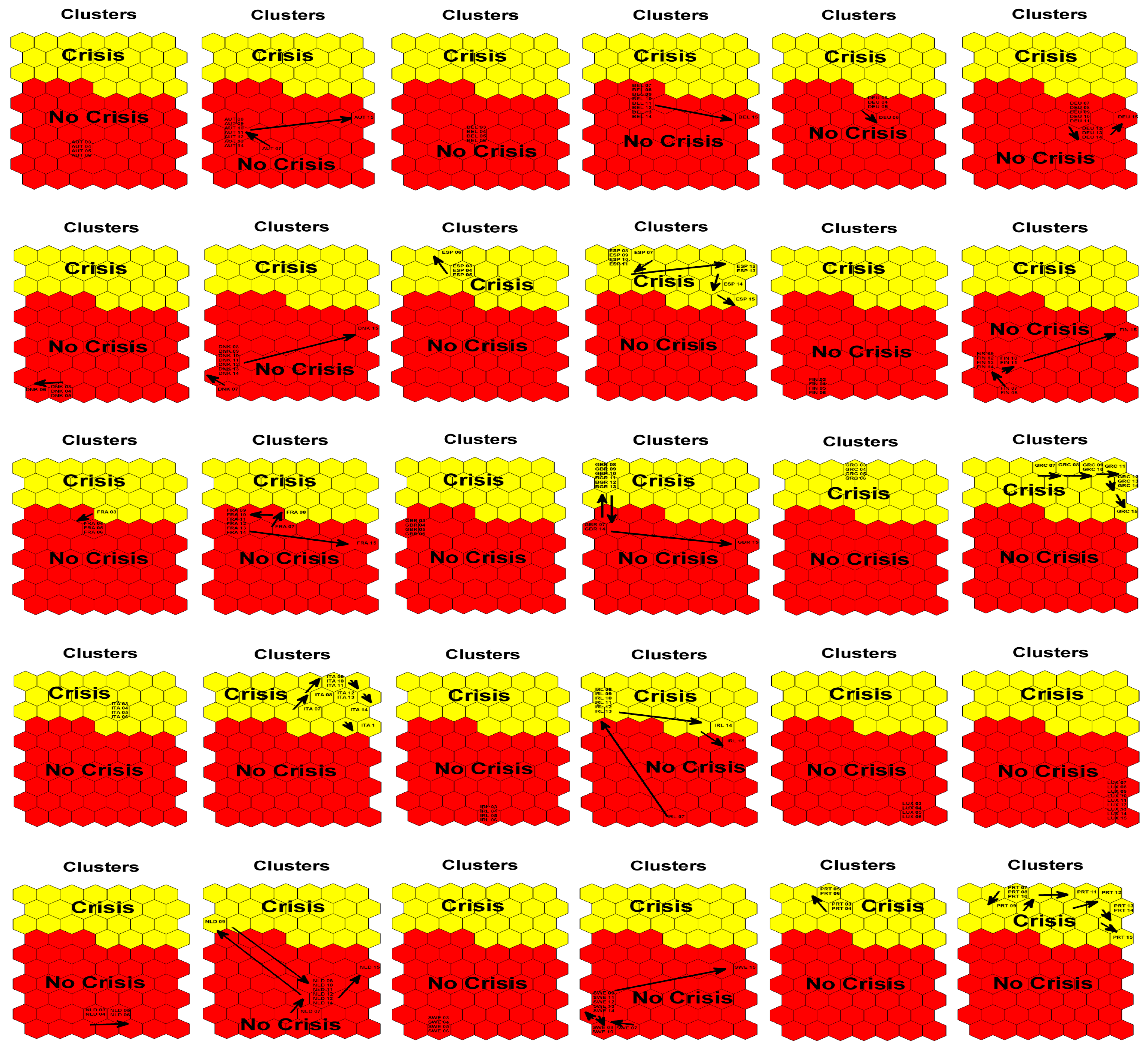
In order to assess the extent to which the EU-15 countries have been affected by the crisis, we present the behavior of their economies on the maps from 2007 to 2015 (see Figure 3). Specifically, we sum up the above Figures and show the transition of EU-15 countries from no crisis to crisis states over time. Strikingly, we see that, when Europe was hit by the global financial crisis in 2007, Greece, Italy, Spain, and Portugal were already in the crisis zone.
The forecast performance results from the SOM estimates are presented in Table 7. The SOM model correctly predict 79.31% of crisis periods and 74% of the no crisis episodes in the EU-15 from 2003 to 2015. Importantly, the model forecasts 100% of crisis episodes for PIIGS countries.
After having obtained the 10 most significant variables that explain the debt crises from the SOM analysis, we estimate a logit model in which the dependent variable is the fiscal stress index reduced to a binary form. Note that the presence of the multicollinearity problem leads us to estimate each indicator separately.
Table 8 shows that all explanatory variables are statistically significant at 1% or 5%. According to the econometric results, increases in budget balance, PSRR, corruption, cash balance, voice and accountability, regulatory quality, GDP growth, rule of law, government effectiveness, and cyclically adjusted balance are associated with lower probabilities of crisis, while increases in NPL/TL and unemployment increase the likelihood of crisis. The results of the econometric analysis are quite similar to the literature. Manasse et al. [34] find that negative domestic developments (low real GDP growth and high inflation rates) and political factors increase the probability of debt crises. Hernandez de Cos et al. [23] find that fiscal balance over GDP and real GDP growth are important determinants of debt crisis. Bruns and Poghosyan [69] and Cerovic et al. [59] find that primary and overall fiscal balance to GDP ratios have a significant impact on debt crisis.
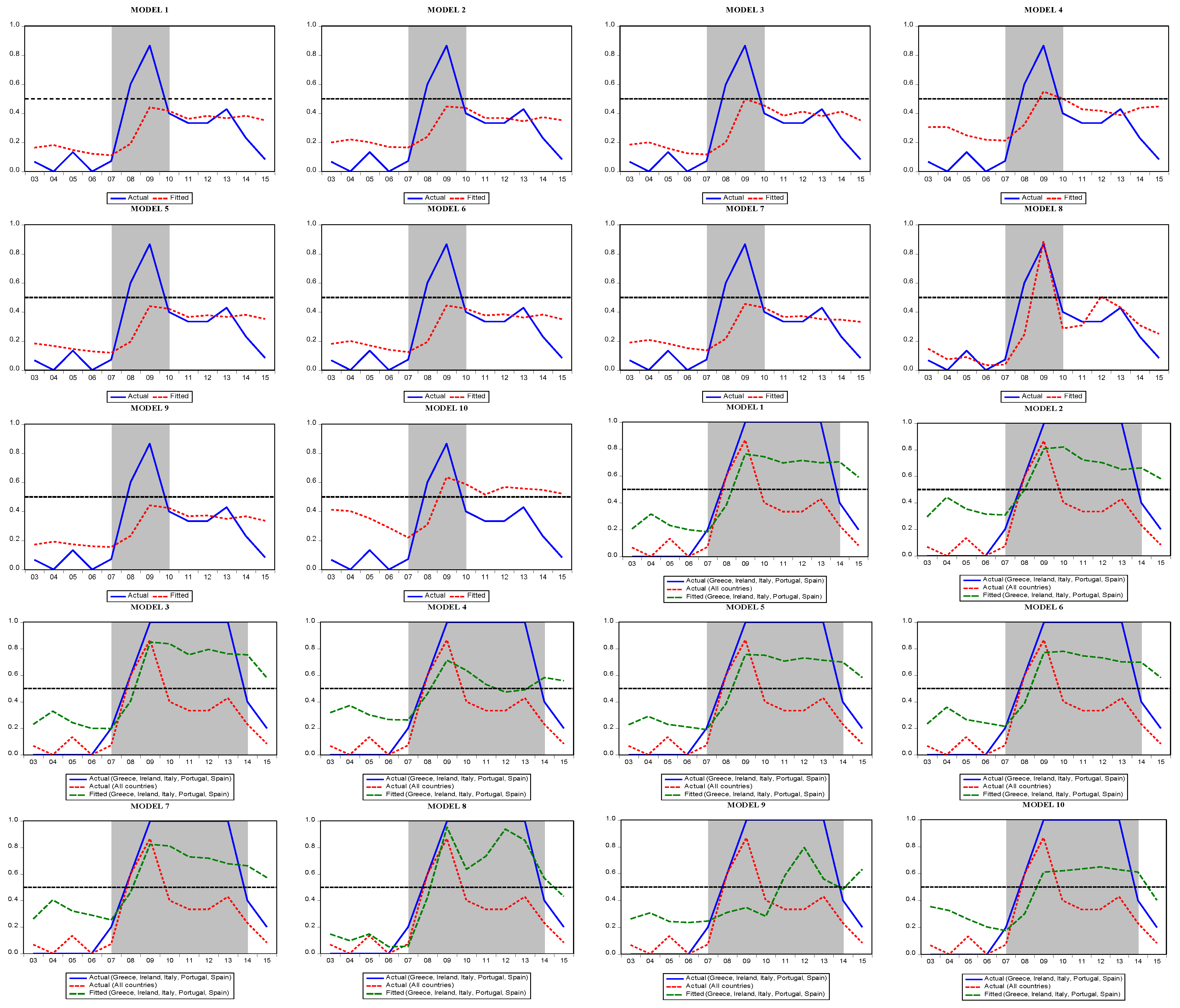
Figure 4 presents the actual and fitted values of the models estimated for the EU-15. We see that, except for Spain, Italy, Greece, Portugal, and Ireland, our studied countries experienced a crisis from 2007 to 2010. As expected, the crisis period was longer for PIIGS countries spanning the period 2007–2014. Table 9 presents the forecast performance matrices for the logit model. Accordingly, the success of the 10 models for predicting crises varies between 50% and 90% for different cut-off values.
In the panel Markov model, the dependent variable (the fiscal stress index) is a continuous variable. To avoid multicollinearity, each variable is estimated separately. Broadly speaking, the results obtained from the Markov approach (Table 10) are similar to those from the logit model. Table 10 suggests that NPL/TL, corruption, cash balance/GDP, voice and accountability, regulatory quality, rule of law, government effectiveness, and cyclically adjusted balance/GDP are statistically significant in only Regime 1, whereas primary balance/GDP, PSRR, unemployment, and GDP growth are statistically significant in Regimes 1 and 2. These results lead us to conclude that the ratios of NPL/TL and unemployment increase the likelihood of crisis, while increases in budget balance, PSRR, corruption, cash balance, voice and accountability, regulatory quality, GDP, and rule of law reduce the likelihood of crisis.
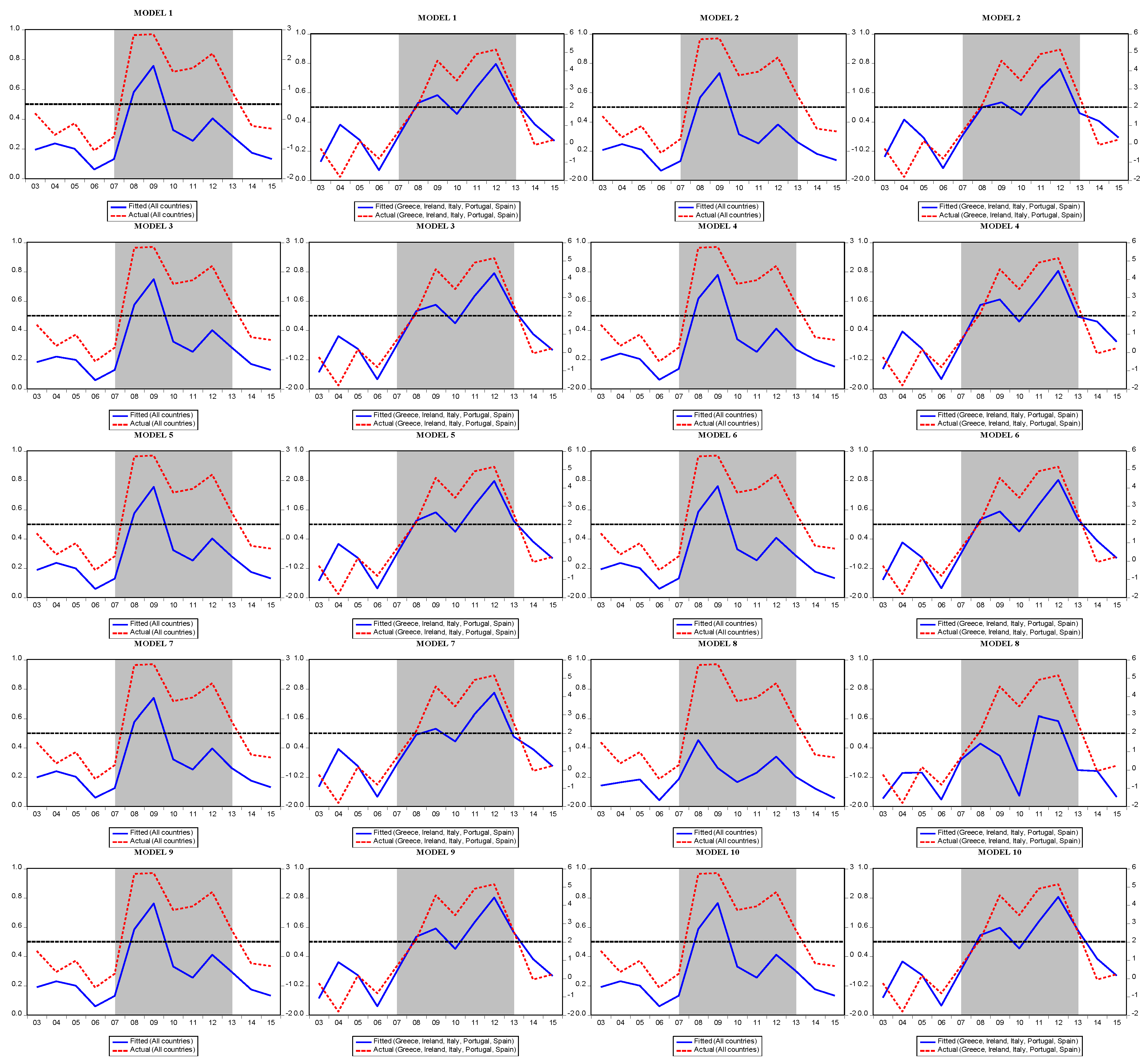
As in the logit model, the Markov model estimates also include the forecast performance of each model and the diagnostic test results. According to the results, there is no normality or autocorrelation problem in the estimated models. In addition, the linearity test shows that using the Markov regime switching model is more appropriate than the linear models. Crisis probabilities obtained from the Markov model are presented separately for the EU-15 and PIIGS. Unlike the logit model, Markov model forecasts show that the crisis started in late 2007 and lasted until 2013, both in PIIGS and the other 10 countries (Figure 5).
The forecast performance results obtained from the panel Markov model are given in Table 11 and Table 12. The models are able to predict, at 0.5 threshold level, all crisis episodes occurred in the EU-15 in the period of 2003–2015 and nearly 80% of no crisis periods. Model test results do not indicate any diagnostic problem and the linearity test results suggest that using nonlinear models such as the Markov and logit is appropriate to predict debt crisis (Table 13).
When we assess the forecast performance of different models, one should note that comparing the results obtained through the SOM with the logit and Markov forecasts can be misleading for two reasons. The first is that SOM uses 51 different leading indicators, while the logit and Markov model employ only 10. The second is that different thresholds cannot be used in the SOM approach. The forecast performance results from SOM show the model can predict crisis periods for the EU-15 more successfully than the no crisis periods. The forecast performance of the logit and Markov models differs according to the selected threshold value. But Markov estimates predict crisis periods more successfully than logit, while logit estimates predict no crisis periods more successfully than the Markov estimates. Markov models could predict approximately 100% of the crisis periods correctly, while the logit model predicted 100% of the no crisis periods (Selecting a lower threshold for both models improves the number of correctly predicted crisis periods but also causes non-crisis periods to be perceived as crises (Type II errors). Markov estimates can be said to have more Type II errors. In contrast, choosing a higher threshold value reduces the number of false alarms but at the expense of increasing the number of missed crises (Type I errors), particularly in logit models).
4. Conclusions
This study aimed to empirically examine the European debt crisis. To do so, we first developed a fiscal stress index contrary for each EU-15 country within the period of 2003–2015, contrary to early empirical papers that tend to use event-based crisis indicators. The empirical results show that our fiscal stress index identifies more ‘debt crisis’ episodes and also indicates a longer crisis period, in particular for the so-called PIIGS, than previous empirical studies applied to debt crises (e.g., [21,22,23]).
As the results obtained from the SOM, Logit, and Markov models are very similar, we propose an overall interpretation. The similarity of the results obtained in all three models is an important indicator of consistency for our analysis. Empirical results obtained from three different models indicate that the debt crisis in the EU-15 is the consequence of the deterioration of both financial and macroeconomic variables such as nonperforming loans over total loans, GDP growth, unemployment rates, primary balance over GDP, and cyclically adjusted balance over GDP. Another interesting point in the estimation results is that despite the similar deterioration in macroeconomic variables, some European countries seem to have exited the crisis very quickly contrary to some countries like Portugal, Italy, Ireland, Spain, or Greece. When comparing these two sets of countries in detail, governance indicators are seen to have played an important role. This situation is observed from the fact that good governance indicators in the SOM, logit, and Markov results significantly reduced the possibility of debt crisis. Greece, Italy, Spain, Portugal, and Ireland, which were deeply affected by the crisis for a longer period, have all poor governance indicators. Therefore, the convergence of countries in terms of governance is very important in addition to economic convergence. Moreover, our logit and Markov models were quite successful in predicting the crisis episodes over the period of 2003–2015. To be more precise, nearly all crisis and no crisis periods in the EU-15 were correctly predicted by our models.
What are the policy implications of our findings? The first one is that constructing the continuous-time fiscal stress index which produces consistent and robust results in identifying fiscal pressure and/or crisis episodes may allow the authorities to take measures to prevent crises. The second one is that governance quality matters both in the outbreak and the length of debt crises. Hence, increasing governance quality could be a significant preventive response to future crises, and the EU may exert pressures on member countries to harmonize governance indicators. Moreover, when we analyze the movements of EU-15 countries over time in terms of macro, financial, and fiscal indicators, we find that there is no homogeneous structure. This can be easily observed from the figures obtained from the SOM analysis, which show the movements of these countries over time: Portugal, Italy, Ireland, Greece and Spain exhibit quite different economic indicators from other countries, not only during the financial and debt crises but also in the pre-crisis period of 2002–2006. Even in the pre-crisis period, these countries’ indicators were quite poor. Therefore, it is important that the countries within the European Union should be similar in terms of macro, financial and fiscal indicators.
Further studies can be carried out to include both a wider time period and a larger country set. In this way, more comprehensive results can be achieved for the constructed fiscal stress index and these results can be presented in a comparable way with previous studies. Furthermore, a very large set of indicators can be used to identify the factors that construct the fiscal stress index; it is thus possible to convert these indicators into the index by methods such as principal component analysis, factor analysis, unobserved components model and budget allocation process.
Author Contributions
Conceptualization, J.-P.A. and R.C.; Methodology, R.C.; Software, R.C.; Validation, J.-P.A. and R.C.; Investigation, R.C.; Data curation, R.C.; Writing—original draft, J.-P.A. and R.C.; Writing—review & editing, J.-P.A. and R.C.; Visualization, R.C.; Supervision, J.-P.A. All authors have read and agreed to the published version of the manuscript.
Funding
This research received no external funding.
Institutional Review Board Statement
Not applicable.
Data Availability Statement
Data published in this paper are available upon request.
Conflicts of Interest
The authors declare no conflict of interest.
References
- Candelon, B.; Palm, F.C. Banking and debt crises in Europe: The dangerous Liaisons? Economist 2010, 158, 81–99. [Google Scholar] [CrossRef] [Green Version]
- Arghyrou, M.G.; Kontonikas, A. The EMU sovereign-debt crisis: Fundamentals, expectations and contagion. J. Int. Financ. Mark. Inst. Money 2012, 22, 658–677. [Google Scholar] [CrossRef] [Green Version]
- De Santis, R.A. The Euro Area Sovereign Debt Crisis: Safe Haven, Credit Rating Agencies and the Spread of the Fever; Working Paper Series 1419; ECB: Frankfurt am Main, Germany, 2012. [Google Scholar]
- Wolf, M. Why the Eurozone Crisis Is Not Over; Peterson Institute for International Economics: Washington, DC, USA, 2012. [Google Scholar]
- De Bruyckere, V.; Gerhardt, M.; Schepens, G.; Vander Vennet, R. Bank/sovereign risk spillovers in the European debt crisis. J. Bank. Financ. 2013, 37, 4793–4809. [Google Scholar] [CrossRef] [Green Version]
- Broto, C.; Perez-Quiros, G. Disentangling contagion among sovereign CDS spreads during the European debt crisis. J. Empir. Financ. 2015, 32, 165–179. [Google Scholar] [CrossRef] [Green Version]
- Calabrese, R.; Elkink, J.A.; Giudici, P.S. Measuring bank contagion in Europe using binary spatial regression models. J. Oper. Res. Soc. 2017, 68, 1503–1511. [Google Scholar] [CrossRef] [Green Version]
- Higgins, M.; Klitgaard, T. Saving imbalances and the euro area sovereign debt crisis. Curr. Issues Econ. Financ. 2011, 17, 52011. [Google Scholar] [CrossRef] [Green Version]
- Uxó, J.; Paúl, J.; Febrero, E. Current account imbalances in the Monetary Union and the Great Recession: Causes and policies. Panoeconomicus 2011, 58, 571–592. [Google Scholar] [CrossRef]
- Knedlik, T.; Von Schweinitz, G. Macroeconomic imbalances as indicators for debt crises in Europe. J. Common Mark. Stud. 2012, 50, 726–745. [Google Scholar] [CrossRef] [Green Version]
- Gros, D. Macroeconomic Imbalances in the Euro Area: Symptom or Cause of the Crisis? CEPS Policy Brief 266; Centre for European Policy Studies: Brussels, Belgium, 2012. [Google Scholar]
- Alessandrini, P.; Fratianni, M.; Hallett, A.H.; Presbitero, A.F. External imbalances and fiscal fragility in the euro area. Open Econ. Rev. 2014, 25, 3–34. [Google Scholar] [CrossRef]
- Brancaccio, E. Current Account Imbalances, the Eurozone Crisis, and a Proposal for a “European Wage Standard”. Int. J. Political Econ. 2012, 41, 47–65. [Google Scholar] [CrossRef] [Green Version]
- Hallett, A.H.; Oliva, J.C.M. The importance of trade and capital imbalances in the European debt crisis. J. Policy Model. 2015, 37, 229–252. [Google Scholar] [CrossRef] [Green Version]
- Mundell, R.A. A theory of optimum currency areas. Am. Econ. Rev. 1961, 51, 657–665. [Google Scholar]
- Ari, A. Introduction. In The European Debt Crisis: Causes, Consequences, Measures and Remedies; Ari, A., Ed.; Cambridge Scholars Publishing: Newcastle upon Tyne, UK, 2014; pp. 1–11. [Google Scholar]
- Berg, A.; Pattillo, C. Predicting currency crises:: The indicators approach and an alternative. J. Int. Money Financ. 1999, 18, 561–586. [Google Scholar] [CrossRef]
- Beckmann, D.; Menkhoff, L.; Sawischlewski, K. Robust lessons about practical early warning systems. J. Policy Model. 2006, 28, 163–193. [Google Scholar] [CrossRef] [Green Version]
- Comelli, F. Comparing parametric and non-parametric early warning systems for currency crises in emerging market economies. Rev. Int. Econ. 2014, 22, 700–721. [Google Scholar] [CrossRef]
- Ari, A.; Cergibozan, R. Currency crises in Turkey: An empirical assessment. Res. Int. Bus. Financ. 2018, 46, 281–293. [Google Scholar] [CrossRef]
- Baldacci, E.; Gabriela, D.; Iva, P.; Samah, M.; Nazim, B. Assessing Fiscal Stress. IMF Working Paper WP/11/100. 2011. Available online: https://www.elibrary.imf.org/doc/IMF001/11797-9781455254316/11797-9781455254316/Other_formats/Source_PDF/11797-9781455253289.pdf (accessed on 1 January 2023).
- Berti, K.; Salto, M.; Lequien, M. An Early-Detection Index of Fiscal Stress for EU Countries (No. 475); Directorate General Economic and Financial Affairs (DG ECFIN), European Commission: Brussels, Belgium, 2012. [Google Scholar]
- Hernández de Cos, P.; Koester, G.B.; Moral-Benito, E.; Nickel, C. Signalling Fiscal Stress in the Euro Area-A Country-Specific Early Warning System; ECB Working Paper, No. 1712; European Central Bank (ECB): Frankfurt, Germany, 2014; ISBN 978-92-899-1120-7. [Google Scholar]
- Sumner, S.P.; Berti, K. A Complementary Tool to Monitor Fiscal Stress in European Economies (No. 049); Directorate General Economic and Financial Affairs (DG ECFIN), European Commission: Brussels, Belgium, 2017. [Google Scholar]
- Detragiache, E.; Spilimbergo, A. Crises and liquidity: Evidence and interpretation. IMF Working Paper WP/1/2. 2001. Available online: https://www.imf.org/en/Publications/WP/Issues/2016/12/30/Crises-and-Liquidity-Evidence-and-Interpretation-3963 (accessed on 1 January 2023).
- McHugh, M.J.; Petrova, I.; Baldacci, M.E. Measuring Fiscal Vulnerability and Fiscal Stress: A Proposed Set of Indicators. IMF Working Paper WP/11/94. 2011. Available online: https://www.imf.org/en/Publications/WP/Issues/2016/12/31/Measuring-Fiscal-Vulnerability-and-Fiscal-Stress-A-Proposed-Set-of-Indicators-24815 (accessed on 1 January 2023).
- Eichengreen, B.; Rose, A.K.; Wyplosz, C. Contagious Currency Crises: First Tests. Scand. J. Econ. 1996, 98, 463–484. [Google Scholar] [CrossRef]
- Kaminsky, G.L.; Reinhart, C.M. The twin crises: The causes of banking and balance-of-payments problems. Am. Econ. Rev. 1999, 89, 473–500. [Google Scholar] [CrossRef] [Green Version]
- Kamin, S.B.; Schindler, J.W.; Samuel, S.L. The Contribution of Domestic and External Factors to Emerging Market Devaluation Crises: An Early Warning Systems Approach; FRB International Finance Discussion Paper, 711; Board of Governors of the Federal Reserve System: Washington, DC, USA, 2001.
- Edison, H.J. Do indicators of financial crises work? An evaluation of an early warning system. Int. J. Financ. Econ. 2003, 8, 11–53. [Google Scholar] [CrossRef] [Green Version]
- Lestano, L.; Jacobs, J.P. Dating currency crises with ad hoc and extreme value-based thresholds: East Asia 1970–2002. Int. J. Financ. Econ. 2007, 12, 371–388. [Google Scholar] [CrossRef]
- Candelon, B.; Dumitrescu, E.I.; Hurlin, C. How to evaluate an early-warning system: Toward a unified statistical framework for assessing financial crises forecasting methods. IMF Econ. Rev. 2012, 60, 75–113. [Google Scholar] [CrossRef]
- Kaminsky, G.; Lizondo, S.; Reinhart, C.M. Leading indicators of currency crises. IMF Staff Pap. 1998, 45, 1–48. [Google Scholar] [CrossRef] [Green Version]
- Manasse, P.; Roubini, N.; Schimmelpfennig, A. Predicting Sovereign Debt Crises. IMF Working Paper WP/03/221. 2003. Available online: https://www.imf.org/en/Publications/WP/Issues/2016/12/30/Predicting-Sovereign-Debt-Crises-16951 (accessed on 1 January 2023).
- Laeven, L.; Valencia, F. Systemic banking crises database. IMF Econ. Rev. 2013, 61, 225–270. [Google Scholar] [CrossRef] [Green Version]
- Laeven, L.; Valencia, F. Systemic Banking Crises Revisited; IMF Working Paper WP/18/206; International Monetary Fund: Washington, DC, USA, 2018. [Google Scholar]
- Guscina, A. Impact of Macroeconomic, Political, and Institutional Factors on the Structure of Government Debt in Emerging Market Countries. IMF Working Paper WP/08/xx. 2008. Available online: https://www.imf.org/en/Publications/WP/Issues/2016/12/31/Impact-of-Macroeconomic-Political-and-Institutional-Factors-on-the-Structure-of-Government-22307 (accessed on 1 January 2023).
- Kaufmann, D.; Kraay, A.; Mastruzzi, M. The worldwide governance indicators: Methodology and analytical issues. Hague J. Rule Law 2011, 3, 220–246. [Google Scholar] [CrossRef]
- Kohonen, T. Self-organized formation of topologically correct feature maps. Biol. Cybern. 1982, 43, 59–69. [Google Scholar] [CrossRef]
- Serrano-Cinca, C. Self organizing neural networks for financial diagnosis. Decis. Support Syst. 1996, 17, 227–238. [Google Scholar] [CrossRef]
- Kiviluoto, K. Predicting bankruptcies with the self-organizing map. Neurocomputing 1998, 21, 191–201. [Google Scholar] [CrossRef]
- Lee, K.; Booth, D.; Alam, P. A comparison of supervised and unsupervised neural networks in predicting bankruptcy of Korean firms. Expert Syst. Appl. 2005, 29, 1–16. [Google Scholar] [CrossRef]
- Shanmuganathan, S.; Sallis, P.; Buckeridge, J. Self-organising map methods in integrated modelling of environmental and economic systems. Environ. Model. Softw. 2006, 21, 1247–1256. [Google Scholar] [CrossRef]
- Giovanis, E. Application of logit model and self-organizing maps (SOMs) for the prediction of financial crisis periods in US economy. J. Financ. Econ. Policy 2010, 2, 98–125. [Google Scholar] [CrossRef]
- Sarlin, P. Exploiting the self-organizing financial stability map. Eng. Appl. Artif. Intell. 2013, 26, 1532–1539. [Google Scholar] [CrossRef]
- Sarlin, P.; Peltonen, T.A. Mapping the state of financial stability. J. Int. Financ. Mark. Inst. Money 2013, 26, 46–76. [Google Scholar] [CrossRef] [Green Version]
- Louis, P.; Seret, A.; Baesens, B. Financial efficiency and social impact of microfinance institutions using self-organizing maps. World Dev. 2013, 46, 197–210. [Google Scholar] [CrossRef]
- Claveria, O.; Monte, E.; Torra, S. A self-organizing map analysis of survey-based agents’ expectations before impending shocks for model selection: The case of the 2008 financial crisis. Int. Econ. 2016, 146, 40–58. [Google Scholar] [CrossRef] [Green Version]
- Deichmann, J.I.; Eshghi, A.; Haughton, D.; Li, M. Socioeconomic Convergence in Europe One Decade After the EU Enlargement of 2004: Application of Self-Organizing Maps. East. Eur. Econ. 2017, 55, 236–260. [Google Scholar] [CrossRef]
- Sarlin, P. Sovereign debt monitor: A visual self-organizing maps approach. In Proceedings of the 2011 IEEE Symposium on Computational Intelligence for Financial Engineering and Economics (CIFEr), Paris, France, 11–15 April 2011; pp. 1–8. [Google Scholar]
- Sarlin, P. Clustering the changing nature of currency crises in emerging markets: An exploration with self-organising maps. Int. J. Comput. Econ. Econom. 2011, 2, 24–46. [Google Scholar] [CrossRef]
- Sarlin, P.; Marghescu, D. Visual predictions of currency crises using self-organizing maps. Intell. Syst. Account. Financ. Manag. 2011, 18, 15–38. [Google Scholar] [CrossRef]
- Ki, S.J.; Lee, S.W.; Kim, J.H. Developing alternative regression models for describing water quality using a self-organizing map. Desalin. Water Treat. 2016, 57, 20146–20158. [Google Scholar] [CrossRef]
- Park, Y.S.; Gevrey, M.; Lek, S.; Giraudel, J.L. Evaluation of relevant species in communities: Development of structuring indices for the classification of communities using a self-organizing map. In Modelling Community Structure in Freshwater Ecosystems; Lek, S., Scardi, M., Verdonschot, P., Descy, J.P., Park, Y.-S., Eds.; Springer: Berlin/Heidelberg, Germany, 2005; pp. 369–380. [Google Scholar]
- Tison, J.; Giraudel, J.L.; Coste, M.; Park, Y.S.; Delmas, F. Use of unsupervised neural networks for ecoregional zoning of hydrosystems through diatom communities: Case study of Adour-Garonne watershed (France). Arch. Hydrobiol. 2004, 159, 409–422. [Google Scholar] [CrossRef]
- Tison, J.; Park, Y.S.; Coste, M.; Wasson, J.G.; Ector, L.; Rimet, F.; Delmas, F. Typology of diatom communities and the influence of hydro-ecoregions: A study on the French hydrosystem scale. Water Res. 2005, 39, 3177–3188. [Google Scholar] [CrossRef]
- Vesanto, J. Data Exploration Process Based on the Self Organizing Map; Acta Polytechnica Scandinavica, Mathematics and Computing Series No. 115; Finnish Academies of Technology: Espoo, Finland, 2002. [Google Scholar]
- Hemming, R.; Kell, M.; Schimmelpfennig, A. Fiscal Vulnerability and Financial Crises in Emerging Market Economies (Vol. 218); International Monetary Fund: Washington, DC, USA, 2003. [Google Scholar]
- Cerovic, M.S.; Gerling, M.K.; Hodge, A.; Medas, P. Predicting Fiscal Crises. IMF Working Paper WP/11/94. 2018. Available online: https://www.imf.org/en/Publications/WP/Issues/2018/08/03/Predicting-Fiscal-Crises-46098 (accessed on 1 January 2023).
- Martinez-Peria, S.M. A regime-switching approach to the study of speculative attacks: A focus on EMS crises. In Advances in Markov-Switching Models; Physica-Verlag HD: Heidelberg, Germany, 2002; pp. 159–194. [Google Scholar]
- Arias, G.; Erlandsson, U.G. Regime Switching as an Alternative Early Warning System of Currency Crises. An Application to South-East Asia; Working Paper; Lund University: Lund, Sweden, 2004. [Google Scholar]
- Alvarez-Plata, P.; Schrooten, M. The Argentinean currency crisis: A Markov-Switching model estimation. Dev. Econ. 2006, 44, 79–91. [Google Scholar] [CrossRef] [Green Version]
- Brunetti, C.; Scotti, C.; Mariano, R.S.; Tan, A.H. Markov switching GARCH models of currency turmoil in Southeast Asia. Emerg. Mark. Rev. 2008, 9, 104–128. [Google Scholar] [CrossRef] [Green Version]
- Abiad, A. Early Warning Systems for Currency Crises: A Regime-Switching Approach. In Hidden Markov Models in Finance. International Series in Operations Research & Management Science; Mamon, R.S., Elliott, R.J., Eds.; Springer: Boston, MA, USA, 2007; Volume 104. [Google Scholar]
- Lopes, J.M.; Nunes, L.C. A Markov regime switching model of crises and contagion: The case of the Iberian countries in the EMS. J. Macroecon. 2012, 34, 1141–1153. [Google Scholar] [CrossRef]
- Pellicer-Chenoll, M.; Garcia-Massó, X.; Morales, J.; Serra-Añó, P.; Solana-Tramunt, M.; González, L.M.; Toca-Herrera, J.L. Physical activity, physical fitness and academic achievement in adolescents: A self-organizing maps approach. Health Educ. Res. 2015, 30, 436–448. [Google Scholar] [CrossRef] [PubMed] [Green Version]
- Chea, R.; Grenouillet, G.; Lek, S. Evidence of water quality degradation in lower Mekong basin revealed by self-organizing map. PLoS ONE 2016, 11, e0145527. [Google Scholar] [CrossRef] [Green Version]
- Gerling, M.K.; Medas, M.P.A.; Poghosyan, M.T.; Farah-Yacoub, J.; Xu, Y. Fiscal Crises. IMF Working Paper WP/17/86. 2017. Available online: https://www.imf.org/en/Publications/WP/Issues/2017/04/03/Fiscal-Crises-44795 (accessed on 1 January 2023).
- Bruns, M.; Poghosyan, T. Leading indicators of fiscal distress: Evidence from extreme bounds analysis. Appl. Econ. 2018, 50, 1454–1478. [Google Scholar] [CrossRef] [Green Version]
Figure 1.
Fiscal stress indexes and their threshold values for EU-15 countries. Note: dashed areas indicate crisis periods.
Figure 1.
Fiscal stress indexes and their threshold values for EU-15 countries. Note: dashed areas indicate crisis periods.

Figure 2.
Net output of a SOM analysis: clusters based on unified distance matrix (U-matrix) and component matrixes.
Figure 2.
Net output of a SOM analysis: clusters based on unified distance matrix (U-matrix) and component matrixes.


Figure 3.
Self-organizing map results for EU-15 countries from 2003–2006 and 2007–2015.

Figure 4.
Predicted probability of crises in the logit models (EU-15 and PIIGS).

Figure 5.
Predicted probability of crisis in the Markov regime switching models.


Table 1.
Optimal cut-off values for EU-15.
| Accuracy Measures | Sensitivity-Specificity Graphic | KLR | ||||||
|---|---|---|---|---|---|---|---|---|
| Country | Cut-Off | Sensitivity | Specificity | Cut-Off | Sensitivity | Specificity | Cut-Off (S) | Cut-Off (G) |
| Austria | 0.410 | 100.0 | 90.90 | 0.410 | 100.0 | 90.90 | 2.535 | 6.381 |
| Belgium | 2.376 | 50.0 | 90.90 | 1.298 | 100.0 | 90.90 | 3.343 | 6.381 |
| Denmark | 0.371 | 100.0 | 81.80 | 2.254 | 100.0 | 100.0 | 4.211 | 6.381 |
| Finland | 1.157 | 100.0 | 91.70 | 3.433 | 100.0 | 100.0 | 4.137 | 6.381 |
| France | 1.035 | 100.0 | 91.70 | 1.788 | 100.0 | 100.0 | 2.161 | 6.381 |
| Germany | 1.218 | 100.0 | 91.70 | 3.516 | 100.0 | 100.0 | 6.157 | 6.381 |
| Greece | 0.154 | 100.0 | 80.0 | 0.752 | 100.0 | 100.0 | 9.407 | 6.381 |
| Ireland | −0.277 | 100.0 | 85.70 | 0.435 | 100.0 | 100.0 | 13.521 | 6.381 |
| Italy | 0.229 | 100.0 | 83.30 | 0.426 | 85.70 | 83.30 | 3.721 | 6.381 |
| Luxembourg | 3.855 | 100.0 | 91.70 | 9.994 | 100.0 | 100.0 | 10.985 | 6.381 |
| Netherlands | 1.058 | 100.0 | 90.90 | 2.523 | 100.0 | 100.0 | 3.972 | 6.381 |
| Portugal | 1.164 | 100.0 | 87.50 | 1.729 | 100.0 | 100.0 | 5.809 | 6.381 |
| Spain | 0.695 | 100.0 | 87.50 | 1.998 | 100.0 | 100.0 | 7.378 | 6.381 |
| Sweden | −0.231 | 100.0 | 90.0 | 0.275 | 100.0 | 100.0 | 2.071 | 6.381 |
| United Kingdom | 0.991 | 100.0 | 90.0 | 1.753 | 100.0 | 100.0 | 3.748 | 6.381 |
Note: S and G indicate optimal threshold values for specific and all EU-15 countries, respectively.
Table 2.
Debt crisis episodes from selected studies.
| Country | Our Results: Crisis Dates | Hernandez de Cos et al. [23]: Crisis Dates | Baldacci et al. [21]: Start of Crisis | Berti et al. [22] |
|---|---|---|---|---|
| Austria | 2009 | No crisis | No crisis | No crisis |
| Belgium | 2003, 2008–2009 | No crisis | No crisis | No crisis |
| Denmark | 2008–2009 | n.a. | No crisis | No crisis |
| Finland | 2009 | No crisis | No crisis | No crisis |
| France | 2009 | No crisis | No crisis | No crisis |
| Germany | 2005 | No crisis | No crisis | No crisis |
| Greece | 2008–2015 | 2008–2010 | 2008 | n.a. |
| Ireland | 2008–2013 | 2008–2010 | 2008 | n.a. |
| Italy | 2007–2014 | 2008–2010 | 2008 | No crisis |
| Luxembourg | 2008 | n.a. | n.a. | No crisis |
| Netherlands | 2008–2009 | No crisis | No crisis | No crisis |
| Portugal | 2009–2013 | 2008, 2010 | 2008, 2010 | 2009–2010 |
| Spain | 2009–2013 | n.a. | 2010 | 2009, 2012 |
| Sweden | 2009, 2013–2014 | n.a. | No crisis | No crisis |
| United Kingdom | 2008–2010 | n.a. | No crisis | 2009 |
Note: “n.a.” indicates that the country is not included in the study.
Table 3.
Descriptive statistics of the dataset.
| INDICATOR | ABBREVIATION | OBS | MIS.VAL. | MEAN | STD.DEV. | MIN | MAX |
|---|---|---|---|---|---|---|---|
| Current account of balance of payments (% of GDP) | CA/GDP 1 | 195 | 0(0%) | 0.94 | 5.48 | −14.43 | 11.93 |
| GDP, real, annual growth | GDP growth 1 | 195 | 0(0%) | 1.17 | 2.82 | −9.17 | 8.40 |
| Exports, goods & services (% of GDP) | X/GDP 1 | 195 | 0(0%) | 54.52 | 39.96 | 18.54 | 213.85 |
| Inflation, consumer prices index (annual %) | Inflation 1 | 195 | 0(0%) | 1.79 | 1.36 | −4.46 | 4.93 |
| Health expenditure, total (% of GDP) | H. Expenditure (Total)/GDP 1 | 180 | 15(7.69%) | 9.52 | 1.20 | 6.80 | 11.97 |
| Unemployment rate (%) | Unemployment 1 | 195 | 0(0%) | 8.46 | 4.65 | 2.33 | 27.51 |
| Government expenditure as % of GDP | GOV.EXP/GDP 1 | 195 | 0(0%) | 48.11 | 5.90 | 32.96 | 65.65 |
| Foreign direct investment, inward, share of GDP | FDI/GDP 1 | 193 | 2(1.02%) | 37.58 | 138.23 | −6.75 | 1144.76 |
| Domestic credit to private sector (% of GDP) | CPS/GDP 1 | 195 | 0(0%) | 110.77 | 35.83 | 54.56 | 202.19 |
| Health expenditure, public (% of government expenditure) | H.EXP (Public)/GOV.EXP 1 | 180 | 15(7.69%) | 15.11 | 2.14 | 9.29 | 20.86 |
| Primary net lending/borrowing (also referred as primary balance) (% of GDP) | Primary Balance/GDP 2 | 195 | 0(0%) | −0.94 | 3.71 | −29.73 | 6.04 |
| Cyclically adjusted balance (% of potential GDP) | Cyclically Adjusted Balance/GDP 2 | 195 | 0(0%) | −2.53 | 3.39 | −18.61 | 4.01 |
| Revenue (% of GDP) | Revenue/GDP 2 | 195 | 0(0%) | 45.03 | 6.18 | 32.79 | 57.44 |
| Reserves, foreign exchange, excluding gold, USD | Reserves 1 | 195 | 0(0%) | 25,169.38 | 24,607.29 | 143.55 | 119,026 |
| Cash surplus/deficit (% of GDP) | Cash Balance/GDP 2 | 179 | 16(8.20%) | −3.51 | 4.23 | −32.37 | 4.11 |
| Tax revenue (% of GDP) | Tax Revenue/GDP 1 | 179 | 16(8.20%) | 22.22 | 5.85 | 0.31 | 35.08 |
| Savings/Expenditures | Savings/Expenditures 1 | 194 | 1(0.51%) | 0.28 | 0.14 | 0.08 | 0.85 |
| Imports, goods & services (% of GDP) | M/GDP 1 | 195 | 0(0%) | 50.45 | 31.81 | 22.92 | 177.65 |
| Trade balance/GDP | Trade/GDP 1 | 195 | 0(0%) | 4.08 | 9.10 | −12.55 | 36.20 |
| External debt, total, share of exports | EX-DEBT/X 1 | 190 | 5(2.56%) | 673.46 | 498.41 | 258.78 | 2807.26 |
| Political stability risk rating (7 = lowest risk) | PSRR 3 | 195 | 0(0%) | 5.81 | 0.62 | 4.26 | 6.83 |
| Credit rating, average | Credit Rating 3 | 195 | 0(0%) | 17.88 | 4.15 | 0.00 | 20.00 |
| Exchange rate, effective real | REER 3 | 195 | 0(0%) | 101.52 | 5.46 | 88.99 | 127.40 |
| External debt, total, share of GDP | EX-DEBT/GDP 1 | 190 | 5(2.56%) | 511.16 | 983.55 | 82.98 | 5490.03 |
| External debt government/GDP | EX-DEBT-GOV/GDP 1 | 179 | 16(8.20%) | 41.96 | 25.61 | 1.65 | 152.47 |
| External debt private/GDP | EX-DEBT-PRIVATE/GDP 1 | 177 | 18 (9.23%) | 214.75 | 195.45 | 33.51 | 1067.07 |
| Foreign direct investment, outward, share of GDP | OFDI/GDP 1 | 182 | 13(6.67%) | 39.26 | 128.79 | −3.95 | 833.68 |
| Wages, hourly, USD | WAGE 3 | 182 | 13(6.67%) | 32.44 | 10.10 | 8.19 | 51.67 |
| Net debt (% of GDP) | NET_DEBT/GDP 2 | 164 | 21(10.77%) | 42.88 | 47.10 | −69.74 | 176.57 |
| Bank capital to assets ratio (%) | CAPITAL/ASSETS 1 | 170 | 25(12.82%) | 5.77 | 1.51 | 3.00 | 13.97 |
| Bank nonperforming loans to total gross loans (%) | NPL/TGL 1 | 187 | 8(4.10%) | 4.58 | 5.93 | 0.08 | 34.67 |
| Trade credit risk rating (7 = lowest risk) | TCRR 3 | 152 | 23(11.79%) | 5.32 | 1.99 | 0.00 | 7.00 |
| Household Debt/GDP | Household Debt/GDP 3 | 125 | 70(35.90%) | 84.16 | 36.15 | 46.78 | 217.51 |
| Control of Corruption | Corruption 1 | 195 | 0(0%) | 1.54 | 0.71 | −0.25 | 2.55 |
| Government Effectiveness | GOV.EFFECT 1 | 195 | 0(0%) | 1.51 | 0.51 | 0.21 | 2.36 |
| Political Stability and Absence of Violence/Terrorism | PSAVTT 1 | 195 | 0(0%) | 0.81 | 0.46 | −0.47 | 1.66 |
| Regulatory Quality | Regulatory Quality 1 | 195 | 0(0%) | 1.43 | 0.38 | 0.34 | 1.92 |
| Rule of Law | Rule of Law 1 | 195 | 0(0%) | 1.49 | 0.48 | 0.24 | 2.12 |
| Voice and Accountability | Voice and Accountability 1 | 195 | 0(0%) | 1.35 | 0.24 | 0.56 | 1.83 |
| Gini coefficient | GINI COEFF 4,5 | 135 | 60(30.77%) | 36.66 | 3.09 | 28.51 | 44.56 |
| Gross enrolment ratio, tertiary, both sexes (%) | Enrolment Tertiary 1 | 156 | 39(20%) | 67.44 | 16.33 | 10.33 | 110.26 |
| Gross enrollment ratio, primary, both sexes (%) | Enrolment Primary 1 | 172 | 23(11.79%) | 103.98 | 4.86 | 95.71 | 120.90 |
| Gross enrolment ratio, secondary, both sexes (%) | Enrolment Secondary 1 | 172 | 23(11.79%) | 110.46 | 13.14 | 91.39 | 164.81 |
| Fertility rate, total (births per woman) | Fertility Rate 1 | 180 | 15(7.69%) | 1.64 | 0.24 | 1.21 | 2.06 |
| Age dependency ratio, old (% of working-age population) | Age Dependency 1 | 195 | 0(0%) | 25.90 | 3.99 | 15.25 | 35.08 |
| Interest payments (% of revenue) | INT_PAY/REVENUE 1 | 195 | 16(8.20%) | 6.77 | 3.79 | 0.27 | 17.29 |
| Interest payments (% of expense) | INT_PAY/EXPENSE 1 | 179 | 16(8.20%) | 6.16 | 3.13 | 0.28 | 14.20 |
| Banking sector leverage | Bank Leverage 1 | 180 | 15(7.69%) | 16.03 | 9.52 | 3.89 | 51.56 |
| M2/GDP | M2/GDP 3 | 182 | 13(6.67%) | 81.31 | 22.09 | 41.62 | 133.32 |
| Fiscal Stress Index | FSI 6 | 195 | 0(0%) | 0.72 | 2.83 | −9.78 | 15.99 |
| Democracy | Democracy 7 | 195 | 0 (0%) | 9.84 | 0.48 | 8.00 | 10.00 |
| Index of Banking Crises (Laeven and Valencia, 2013) | Banking Crises | 195 | 0(0%) | 0.58 | 0.49 | 0.00 | 1.00 |
Note: Obs, Mis. Val, M, Min and Max denote observations, missing value, mean, minimum and maximum, respectively, while 1, 2, 3, 4, 5, 6, and 7 indicate World Bank, International Monetary Fund, Oxford Economics, World Income Inequality Database, and Standardized World Income Inequality.
Table 4.
Self-organizing map-based cluster results.
| VARIABLES | NO CRISIS (M) | CRISIS (M) | NO CRISIS (SD) | CRISIS (SD) |
|---|---|---|---|---|
| Frequency (%) | 64.290 | 35.710 | 64.290 | 35.710 |
| CA/GDP | 3.566 | −3.874 | 3.852 | 4.569 |
| GDP Growth | 1.754 | 0.066 | 2.527 | 3.017 |
| X/GDP | 64.514 | 35.858 | 43.348 | 23.399 |
| Inflation | 1.725 | 1.918 | 1.125 | 1.711 |
| H. Expenditure (Total)/GDP | 9.547 | 9.475 | 1.109 | 1.345 |
| Unemployment | 6.705 | 11.762 | 2.009 | 6.175 |
| GOV.EXP/GDP | 48.450 | 47.522 | 6.285 | 5.095 |
| FDI/GDP | 55.846 | 3.998 | 169.145 | 6.140 |
| CPS/GDP | 104.953 | 121.710 | 34.557 | 35.854 |
| H.EXP (Public)/GOV.EXP | 15.651 | 14.096 | 2.0931 | 1.941 |
| Primary Balance/GDP | 0.115 | −2.949 | 2.264 | 4.919 |
| Cyclically Adjusted Balance/GDP | −1.184 | −5.046 | 2.289 | 3.683 |
| Revenue/GDP | 47.309 | 40.774 | 5.796 | 4.403 |
| Reserves | 27,640.150 | 20,564.050 | 24,962.110 | 23,407.870 |
| Cash Balance/GDP | −1.956 | −6.317 | 2.271 | 5.378 |
| Tax Revenue/GDP | 23.469 | 19.660 | 5.451 | 6.406 |
| Savings/Expenditures | 0.308 | 0.218 | 0.147 | 0.117 |
| M/GDP | 57.648 | 36.955 | 35.300 | 17.497 |
| Trade/GDP | 6.866 | −1.097 | 8.773 | 7.232 |
| EX-DEBT/X | 674.356 | 670.413 | 588.113 | 269.289 |
| PSRR | 6.154 | 5.171 | 0.303 | 0.530 |
| Credit Rating | 19.254 | 15.310 | 3.091 | 4.645 |
| REER | 102.214 | 100.212 | 6.097 | 3.733 |
| EX-DEBT/GDP | 644.485 | 266.116 | 1188.315 | 257.153 |
| EX-DEBT-GOV/GDP | 34.552 | 54.269 | 19.030 | 30.138 |
| EX-DEBT-PRIVATE/GDP | 216.908 | 211.008 | 149.895 | 254.582 |
| OFDI/GDP | 60.280 | 4.005 | 159.224 | 6.483 |
| WAGE | 37.241 | 24.375 | 6.667 | 9.795 |
| NET_DEBT/GDP | 23.572 | 77.249 | 40.604 | 37.454 |
| CAPITAL/ASSETS | 5.532 | 6.149 | 1.567 | 1.330 |
| NPL/TGL | 2.177 | 8.817 | 1.874 | 7.942 |
| TCRR | 5.945 | 4.367 | 1.708 | 2.025 |
| Household Debt/GDP | 71.747 | 108.856 | 27.480 | 39.372 |
| Corruption | 1.922 | 0.817 | 0.367 | 0.631 |
| GOV.EFFECT | 1.790 | 0.981 | 0.246 | 0.445 |
| PSAVTT | 1.011 | 0.421 | 0.333 | 0.423 |
| Regulatory Quality | 1.615 | 1.082 | 0.218 | 0.378 |
| Rule of Law | 1.752 | 1.014 | 0.213 | 0.476 |
| Voice and Accountability | 1.483 | 1.109 | 0.138 | 0.205 |
| GINI COEFF | 35.677 | 38.523 | 2.752 | 2.888 |
| Enrollment Tertiary | 66.145 | 69.360 | 17.513 | 13.812 |
| Enrollment Primary | 103.028 | 105.829 | 4.228 | 5.458 |
| Enrollment Secondary | 111.447 | 108.453 | 14.072 | 11.030 |
| Fertility Rate | 1.714 | 1.508 | 0.197 | 0.266 |
| Age Dependency | 25.413 | 26.806 | 3.725 | 4.334 |
| INT_PAY/REVENUE | 4.695 | 10.524 | 2.241 | 3.072 |
| INT_PAY/EXPENSE | 4.571 | 9.026 | 2.100 | 2.607 |
| Bank Leverage | 15.474 | 17.058 | 8.312 | 11.362 |
| M2/GDP | 77.711 | 87.144 | 23.254 | 18.801 |
| FSI | 0.038 | 1.981 | 2.394 | 3.154 |
| Democracy | 9.772 | 9.971 | 0.566 | 0.170 |
| Banking Crises | 0.520 | 0.691 | 0.502 | 0.465 |
Table 5.
List of significant variables ranked based on four indexes (SI—structuring index, RI—relative importance, CD—cluster description, and SRC—Spearman’s rank correlation) in a SOM.
Table 5.
List of significant variables ranked based on four indexes (SI—structuring index, RI—relative importance, CD—cluster description, and SRC—Spearman’s rank correlation) in a SOM.
| Rank | SI | Values | RI | Values | CD | Values | SRC | Values |
|---|---|---|---|---|---|---|---|---|
| 1 | GOV.EFFECT | 1328.206 | Primary Balance/GDP | 2.487 | NPL/TGL | 4.238 | GDP growth | −0.639 *** |
| 2 | PSRR | 1320.574 | EX-DEBT-GOV/GDP | 2.370 | Unemployment | 3.074 | Primary Balance/GDP | −0.527 *** |
| 3 | Voice and Accountability | 1313.764 | PSRR | 2.347 | Cash Balance/GDP | 2.368 | Cash Balance/GDP | −0.428 *** |
| 4 | Rule of Law | 1313.293 | Corruption | 2.329 | Rule of Law | 2.235 | Cyclically Adjusted Balance/GDP | −0.398 *** |
| 5 | Corruption | 1310.869 | NET_DEBT/GDP | 2.283 | Primary Balance/GDP | 2.173 | NPL/TGL | 0.386 *** |
| 6 | Regulatory Quality | 1282.465 | Unemployment | 2.231 | GOV.EFFECT | 1.805 | Banking Crises | 0.373 *** |
| 7 | CA/GDP | 1241.308 | Regulatory Quality | 2.194 | PSRR | 1.746 | EX-DEBT/X | 0.341 *** |
| 8 | INT_PAY/REVENUE | 1215.579 | M2/GDP | 2.194 | Regulatory Quality | 1.736 | CA/GDP | −0.324 *** |
| 9 | PSAVTT | 1192.348 | CAPITAL/ASSET | 2.182 | Corruption | 1.722 | Bank Leverage | 0.323 *** |
| 10 | INT_PAY/EXPENSE | 1176.359 | INT_PAY/EXPENSE | 2.181 | EX-DEBT-PRIVATE/GDP | 1.698 | GOV.EFFECT | −0.313 *** |
| 11 | NET_DEBT/GDP | 1097.219 | Cash Balance/GDP | 2.168 | Cyclically Adjusted Balance/GDP | 1.609 | PSRR | −0.306 *** |
| 12 | Trade/GDP | 1048.616 | GINI COEFF | 2.136 | EX-DEBT-GOV/GDP | 1.584 | Voice and Accountability | −0.302 *** |
| 13 | Age Dependency | 1023.416 | Reserves | 2.132 | Inflation | 1.522 | NET_DEBT/GDP | 0.302 *** |
| 14 | Cyclically Adjusted Balance/GDP | 992.023 | Enrollment Tertiary | 2.131 | Credit Rating | 1.503 | Savings/Expenditures | −0.295 *** |
| 15 | WAGE | 983.387 | CPS/GDP | 2.127 | Voice and Accountability | 1.491 | EX-DEBT-GOV/GDP | 0.280 *** |
| 16 | Revenue/GDP | 927.769 | Bank Leverage | 2.120 | WAGE | 1.469 | INT_PAY/REVENUE | 0.269 *** |
| 17 | Enrollment Tertiary | 927.575 | Banking Crises | 2.114 | Household Debt/GDP | 1.433 | Rule of Law | −0.268 *** |
| 18 | NPL/TGL | 926.662 | Voice and Accountability | 2.097 | INT_PAY/REVENUE | 1.371 | TCRR | −0.267 *** |
| 19 | Unemployment | 908.386 | GDP growth | 2.085 | Bank Leverage | 1.367 | Trade/GDP | −0.262 *** |
| 20 | X/GDP | 907.778 | EX-DEBT/GDP | 2.078 | Fertility Rate | 1.350 | OFDI/GDP | −0.260 *** |
| 21 | Tax Revenue/GDP | 904.0651 | Trade/GDP | 2.057 | FSI | 1.317 | Corruption | −0.255 *** |
| 22 | Fertility Rate | 892.051 | Enrollment Secondary | 2.046 | Enrollment Primary | 1.291 | Credit Rating | −0.255 *** |
| 23 | M/GDP | 868.569 | NPL/TGL | 2.016 | PSAVTT | 1.270 | M2/GDP | 0.249 *** |
| 24 | Cash Balance/GDP | 865.003 | FDI/GDP | 1.98 | INT_PAY/EXPENSE | 1.242 | PSAVTT | −0.247 *** |
| 25 | Democracy | 853.076 | TCRR | 1.977 | H. Expenditure (Total)/GDP | 1.213 | Household Debt/GDP | 0.231 *** |
| 26 | EX-DEBT-GOV/GDP | 852.431 | H.EXP (Public)/GOV.EXP | 1.917 | GDP growth | 1.194 | Unemployment | 0.229 *** |
| 27 | GOV.EXP/GDP | 833.429 | H. Expenditure (Total)/GDP | 1.908 | CA/GDP | 1.186 | GOV.EXP/GDP | 0.223 *** |
| 28 | EX-DEBT/X | 822.099 | Inflation | 1.903 | TCRR | 1.185 | Regulatory Quality | −0.211 *** |
| 29 | M2/GDP | 813.392 | OFDI/GDP | 1.881 | Tax Revenue/GDP | 1.175 | X/GDP | −0.192 *** |
| 30 | Credit Rating | 810.121 | Enrollment Primary | 1.873 | Age Dependency | 1.163 | Enrolment Primary | 0.186 ** |
| 31 | Banking Crises | 787.017 | Age Dependency | 1.854 | GINI COEFF | 1.045 | M/GDP | −0.173 ** |
| 32 | H. Expenditure (Total)/GDP | 774.519 | Tax Revenue/GDP | 1.849 | CPS/GDP | 1.038 | INT_PAY/EXPENSE | 0.171 ** |
| 33 | Savings/Expenditures | 761.388 | Cyclically Adjusted Balance/GDP | 1.847 | Reserves | 0.938 | GINI COEFF | 0.166 * |
| 34 | Bank Leverage | 756.183 | Revenue/GDP | 1.835 | Banking Crises | 0.928 | EX-DEBT/GDP | 0.153 ** |
| 35 | EX-DEBT-PRIVATE/GDP | 756.152 | REER | 1.829 | H.EXP (Public)/GOV.EXP | 0.927 | Revenue/GDP | −0.152 ** |
| 36 | CPS/GDP | 738.579 | CA/GDP | 1.801 | NET_DEBT/GDP | 0.922 | H.EXP (Public)/GOV.EXP | −0.140 * |
| 37 | GINI COEFF | 712.864 | Household Debt/GDP | 1.791 | CAPITAL/ASSETS | 0.849 | Age Dependency | 0.105 |
| 38 | Reserves | 707.545 | Credit Rating | 1.759 | Trade/GDP | 0.824 | Tax Revenue/GDP | −0.103 |
| 39 | H.EXP (Public)/GOV.EXP | 700.329 | Fertility Rate | 1.755 | GOV.EXP/GDP | 0.811 | FDI/GDP | −0.101 |
| 40 | Enrollment Secondary | 683.320 | GOV.EXP/GDP | 1.745 | M2/GDP | 0.809 | CPS/GDP | 0.090 |
| 41 | Primary Balance/GDP | 682.901 | Rule of Law | 1.735 | Savings/Expenditures | 0.793 | H. Expenditure (Total)/GDP | 0.087 |
| 42 | Enrollment Primary | 667.923 | X/GDP | 1.730 | Enrollment Tertiary | 0.789 | Reserves | −0.071 |
| 43 | EX-DEBT/GDP | 647.172 | PSAVTT | 1.691 | Enrollment Secondary | 0.784 | Enrollment Secondary | 0.061 |
| 44 | GDP growth | 642.788 | GOV.EFFECT | 1.672 | Revenue/GDP | 0.760 | CAPITAL/ASSET | −0.059 |
| 45 | CAPITAL/ASSETS | 638.174 | EX-DEBT/X | 1.551 | REER | 0.612 | WAGE | −0.058 |
| 46 | FSI | 615.079 | FSI | 1.541 | X/GDP | 0.540 | Fertility Rate | −0.058 |
| 47 | TCRR | 611.866 | INT_PAY/REVENUE | 1.497 | M/GDP | 0.496 | EX-DEBT-PRIVATE/GDP | 0.034 |
| 48 | Inflation | 608.657 | Savings/Expenditures | 1.488 | EX-DEBT/X | 0.458 | REER | 0.024 |
| 49 | Household Debt/GDP | 567.960 | M/GDP | 1.477 | Democracy | 0.301 | Democracy | −0.026 |
| 50 | REER | 564.612 | Democracy | 1.473 | EX-DEBT/GDP | 0.216 | Enrollment Tertiary | −0.020 |
| 51 | OFDI/GDP | 531.554 | WAGE | 1.341 | OFDI/GDP | 0.041 | Inflation | 0.012 |
| 52 | FDI/GDP | 484.981 | EX-DEBT-PRIVATE/GDP | 1.193 | FDI/GDP | 0.036 |
Note: ***, ** and * represent statistical significance at the 1%, 5% and 10% level, respectively.
Table 6.
List of significant variables ranked based on SRC (crisis and non-crisis periods)—Spearman’s rank correlation and overall indexes) in a SOM.
Table 6.
List of significant variables ranked based on SRC (crisis and non-crisis periods)—Spearman’s rank correlation and overall indexes) in a SOM.
| Rank | SRC (Crisis) | Values | SRC (No Crisis) | Values | Overall Index (1) | Values | Overall Index (2) | Values |
|---|---|---|---|---|---|---|---|---|
| 1 | GDP growth | −0.752 *** | Primary Balance/GDP | −0.543 *** | NPL/TGL | 14.112 | NPL/TGL | 5.992 |
| 2 | Banking Crises | 0.547 *** | GDP growth | −0.510 *** | Primary Balance/GDP | 12.135 | Primary Balance/GDP | 4.780 |
| 3 | Household Debt/GDP | 0.516 *** | Cyclically Adjusted Balance/GDP | −0.315 ** | Cash Balance/GDP | 11.617 | PSRR | 4.769 |
| 4 | EXDEBT/GDP | 0.512 *** | Cash Balance/GDP | −0.284 *** | GDP growth | 11.148 | Corruption | 4.257 |
| 5 | EXDEBT/X | 0.490 *** | Bank Leverage | 0.263 *** | Unemployment | 11.059 | Cash Balance/GDP | 3.969 |
| 6 | Primary Balance/GDP | −0.476 *** | Trade/GDP | −0.259 *** | PSRR | 10.725 | Unemployment | 3.902 |
| 7 | GOV.EXP/GDP | 0.471 *** | WAGE | 0.251 *** | Rule of Law | 10.508 | Voice and Accountability | 3.472 |
| 8 | Bank Leverage | 0.459 *** | Banking Crises | 0.251 *** | GOV.EFFECT | 10.221 | Regulatory Quality | 3.357 |
| 9 | EXDEBTPRIVATE/GDP | 0.401 *** | EXDEBT/X | 0.239 *** | Corruption | 10.185 | Rule of Law | 2.978 |
| 10 | M2/GDP | 0.393 *** | GOV.EXP/GDP | 0.238 *** | Cyclically Adjusted Balance/GDP | 10.128 | GDP growth | 2.645 |
| 11 | Cash Balance/GDP | −0.333 *** | GINI COEFF | 0.215 ** | Voice and Accountability | 10.029 | GOV.EFFECT | 2.548 |
| 12 | NPL/TGL | 0.320 *** | Savings/Expenditures | −0.194 ** | Regulatory Quality | 9.609 | EX-DEBT-GOV/GDP | 2.453 |
| 13 | Savings/Expenditures | −0.314 *** | CA/GDP | −0.192 ** | CA/GDP | 9.302 | NET_DEBT/GDP | 2.420 |
| 14 | Enrollment Secondary | 0.305 ** | NPL/TGL | 0.192 ** | EX-DEBT-GOV/GDP | 9.234 | Cyclically Adjusted Balance/GDP | 2.094 |
| 15 | X/GDP | 0.302 ** | EXDEBTGOV/GDP | 0.172 * | NET_DEBT/GDP | 8.860 | INT_PAY/EXPENSE | 1.880 |
| 16 | Cyclically Adjusted Balance/GDP | −0.264 * | CAPITAL/ASSETS | −0.161 * | Bank Leverage | 8.828 | CA/GDP | 1.855 |
| 17 | GINI COEFF | −0.262 ** | FSI | 1 | INT_PAY/REVENUE | 8.728 | Bank Leverage | 1.174 |
| 18 | Unemployment | 0.260 ** | Democracy | −0.156 | Banking Crises | 8.665 | Banking Crises | 1.038 |
| 19 | Credit Rating | −0.240 ** | X/GDP | −0.145 | PSAVTT | 8.515 | Trade/GDP | 0.985 |
| 20 | EXDEBTGOV/GDP | 0.239 ** | OFDI/GDP | −0.145 | INT_PAY/EXPENSE | 8.236 | PSAVTT | 0.811 |
| 21 | Fertility Rate | 0.226 * | EXDEBT/GDP | 0.139 | Credit Rating | 8.178 | INT_PAY/REVENUE | 0.526 |
| 22 | CAPITAL/ASSETS | −0.220 * | M2/GDP | 0.117 | Trade/GDP | 8.012 | M2/GDP | 0.358 |
| 23 | M/GDP | 0.211 * | TCRR | −0.100 | TCRR | 7.578 | Credit Rating | −0.182 |
| 24 | INT_PAY/EXPENSE | −0.210 * | Tax Revenue/GDP | −0.099 | M2/GDP | 7.492 | Age Dependency | −0.517 |
| 25 | FSI | 1 | H. Expenditure (Total)/GDP | 0.097 | Household Debt/GDP | 7.352 | GINI COEFF | −0.551 |
| 26 | Inflation | −0.188 | M/GDP | −0.094 | EX-DEBT/X | 7.161 | TCRR | −0.606 |
| 27 | Trade/GDP | 0.173 | Enrollment Primary | −0.093 | Savings/Expenditures | 7.065 | Tax Revenue/GDP | −1.037 |
| 28 | WAGE | 0.171 | PSAVTT | −0.085 | Enrollment Primary | 7.025 | CPS/GDP | −1.041 |
| 29 | OFDI/GDP | −0.168 | Enrollment Tertiary | 0.085 | GOV.EXP/GDP | 6.854 | Enrollment Tertiary | −1.087 |
| 30 | H.EXP (Public)/GOV.EXP | −0.162 | Rule of Law | −0.068 | Age Dependency | 6.852 | Enrollment Primary | −1.182 |
| 31 | H. Expenditure (Total)/GDP | 0.157 | Unemployment | 0.065 | GINI COEFF | 6.824 | Revenue/GDP | −1.206 |
| 32 | Reserves | −0.152 | Reserves | 0.062 | Tax Revenue/GDP | 6.585 | GOV.EXP/GDP | −1.332 |
| 33 | Tax Revenue/GDP | 0.142 | NET_DEBT/GDP | 0.062 | Revenue/GDP | 6.427 | Household Debt/GDP | −1.367 |
| 34 | REER | 0.140 | INT_PAY/REVENUE | 0.057 | Fertility Rate | 6.327 | Reserves | −1.433 |
| 35 | CPS/GDP | 0.135 | FDI/GDP | −0.057 | X/GDP | 6.301 | H. Expenditure (Total)/GDP | −1.441 |
| 36 | NET_DEBT/GDP | 0.119 | Voice and Accountability | −0.056 | WAGE | 6.297 | Fertility Rate | −1.506 |
| 37 | Enrollment Primary | 0.117 | REER | 0.053 | H. Expenditure (Total)/GDP | 6.274 | X/GDP | −1.676 |
| 38 | Regulatory Quality | −0.109 | Age Dependency | 0.052 | CPS/GDP | 6.170 | EX-DEBT/X | −1.694 |
| 39 | Enrollment Tertiary | 0.084 | Household Debt/GDP | −0.051 | H.EXP (Public)/GOV.EXP | 6.159 | H.EXP (Public)/GOV.EXP | −1.734 |
| 40 | Rule of Law | 0.078 | GOV.EFFECT | −0.049 | EX-DEBT-PRIVATE/GDP | 5.787 | CAPITAL/ASSET | −1.762 |
| 41 | Voice and Accountability | −0.07 | Enrollment Secondary | 0.048 | Reserves | 5.780 | Savings/Expenditures | −2.043 |
| 42 | FDI/GDP | 0.052 | EXDEBTPRIVATE/GDP | 0.048 | M/GDP | 5.721 | Enrollment Secondary | −2.128 |
| 43 | CA/GDP | 0.049 | H.EXP (Public)/GOV.EXP | 0.041 | Inflation | 5.701 | Inflation | −2.279 |
| 44 | INT_PAY/REVENUE | 0.032 | CPS/GDP | −0.040 | Enrollment Tertiary | 5.568 | EX-DEBT/GDP | −2.285 |
| 45 | TCRR | −0.031 | PSRR | −0.036 | OFDI/GDP | 5.473 | WAGE | −2.418 |
| 46 | Revenue/GDP | −0.027 | Inflation | 0.034 | CAPITAL/ASSET | 5.431 | OFDI/GDP | −2.931 |
| 47 | Age Dependency | 0.021 | Regulatory Quality | 0.033 | Enrollment Secondary | 5.312 | M/GDP | −2.937 |
| 48 | Corruption | 0.013 | Fertility Rate | −0.027 | EX-DEBT/GDP | 5.222 | EX-DEBT-PRIVATE/GDP | −3.759 |
| 49 | GOV.EFFECT | −0.012 | Revenue/GDP | 0.024 | FSI | 4.927 | FSI | −3.906 |
| 50 | PSRR | 0.005 | Corruption | −0.016 | REER | 4.232 | REER | −3.908 |
| 51 | PSAVTT | 0.005 | INT_PAY/EXPENSE | −0.012 | Democracy | 4.046 | FDI/GDP | −3.950 |
| 52 | Democracy | 0.004 | Credit Rating | 0.010 | FDI/GDP | 4.017 | Democracy | −4.365 |
Note: ***, ** and * represent statistical significance at the 1%, 5% and 10% level, respectively.
Table 7.
Forecast performance of SOM.
| Criteria | Model (EU-15) | Model (PIIGS) |
|---|---|---|
| % and number of correctly predicted non-crises | 79.31% (115/145) | 18.18% (6/33) |
| % and number of correctly predicted crises | 74.00% (37/50) | 100% (32/32) |
Table 8.
Logit estimation results.
| Dependent Variable: FSI | ||||||||||
|---|---|---|---|---|---|---|---|---|---|---|
| Variables | Model 1 | Model 2 | Model 3 | Model 4 | Model 5 | Model 6 | Model 7 | Model 8 | Model 9 | Model 10 |
| NPL/TGL | 0.150 *** (0.038) | 0.063 ** (0.028) | 0.167 *** (0.052) | 0.164 *** (0.052) | 0.131 *** (0.036) | 0.108 *** (0.033) | 0.096 *** (0.031) | 0.168 *** (0.050) | 0.093 *** (0.030) | 0.175 *** (0.042) |
| Primary Balance/GDP | −0.280 *** (0.071) | −0.251 *** (0.1348) | −0.153 * (0.081) | −0.277 *** (0.073) | −0.265 *** (0.069) | −0.266 *** (0.069) | −0.285 *** (0.071) | −0.162 ** (0.083) | −0.259 *** (0.070) | −0.249 ** (0.103) |
| PSRR | −0.375 *** (0.052) | |||||||||
| Corruption | −1.094 *** (0.153) | |||||||||
| Cash Balance/GDP | −0.173 ** (0.076) | |||||||||
| Unemployment | 0.024 *** (0.004) | |||||||||
| Voice and Accountability | −1.537 *** (0.211) | |||||||||
| Regulatory Quality | −1.361 *** (0.187) | |||||||||
| Rule of Law | −1.296 *** (0.178) | |||||||||
| GDP growth | −0.612 *** (0.123) | |||||||||
| GOV.EFFECT | −1.260 *** (0.174) | |||||||||
| Cyclically Adjusted Balance/GDP | −0.165 *** (0.039) | |||||||||
| CONSTANT | 1.323 (2.335) | −1.541 ** (0.697) | −2.605 *** (0.374) | −2.390 *** (0.428) | −0.047 (1.613) | −1.240 (0.999) | −0.913 (0.814) | −1.713 *** (0.366) | −0.985 (0.829) | −2.333 *** (0.351) |
| Observations | 195 | 195 | 195 | 195 | 195 | 195 | 195 | 195 | 195 | 195 |
| Pseudo R2 | 0.27 | 0.26 | 0.30 | 0.26 | 0.27 | 0.26 | 0.27 | 0.45 | 0.27 | 0.26 |
| LR Stat | 59.4 *** | 58.4 *** | 63.7 *** | 57.4 *** | 59.0 *** | 58.2 *** | 60.0 *** | 99.7 *** | 59.6 *** | 57.4 *** |
| Akaike Info | 0.91 | 0.91 | 0.89 | 0.92 | 0.91 | 0.91 | 0.90 | 0.69 | 0.91 | 0.92 |
Note: ***, ** and * represent statistical significance at the 1%, 5% and 10% level, respectively. The values in parentheses are standard deviations.
Table 9.
Forecast performance of logit models.
| Cut-Off Level | Model 1 | Model 2 | Model 3 | Model 4 | Model 5 | Model 6 | Model 7 | Model 8 | Model 9 | Model 10 |
|---|---|---|---|---|---|---|---|---|---|---|
| C = 0.5 | ||||||||||
| % and number of correctly predicted non-crises | 95.10% (136/143) | 93.71% (134/143) | 95.10% (136/143) | 83.22% (119/143) | 95.10% (136/143) | 95.10% (136/143) | 95.10% (136/143) | 97.20% (139/143) | 93.71% (134/143) | 66.43% (95/143) |
| % and number of correctly predicted crises | 50% (26/52) | 55.77% (29/52) | 57.69% (30/52) | 51.92% (27/52) | 50% (26/52) | 55.77% (29/52) | 55.77% (29/52) | 67.31% (35/52) | 55.77% (29/52) | 53.85% (28/52) |
| C = 0.25 | ||||||||||
| % and number of correctly predicted non-crises | 76.22% (109/143) | 74.83% (107/143) | 85.52% (118/143) | 40.56% (58/143) | 75.52% (108/143) | 72.03% (103/143) | 76.22% (109/143) | 85.31% (122/143) | 75.52% (108/143) | 21.68% (31/143) |
| % and number of correctly predicted crises | 69.23% (36/52) | 73.08% (38/52) | 75% (39/52) | 76.92% (40/52) | 69.23% (36/52) | 69.23% (36/52) | 73.08% (38/52) | 78.85% (41/52) | 73.08% (38/52) | 88.46% (46/52) |
| C = 0.2 | ||||||||||
| % and number of correctly predicted non-crises | 68.53% (98/143) | 66.43% (95/143) | 72.72% (104/143) | 34.27% (49/143) | 67.83% (97/143) | 69.93% (100/143) | 65.73% (94/143) | 78.32% (112/143) | 69.93% (100/143) | 13.94% (20/143) |
| % and number of correctly predicted crises | 76.92% (40/52) | 75% (39/52) | 76.92% (40/52) | 88.46% (46/52) | 75% (39/52) | 73.08% (38/52) | 75% (39/52) | 78.85% (41/52) | 76.92% (40/52) | 90.38% (47/52) |
Table 10.
Markov Estimation Results.
| Variables | Model 1 | Model 2 | Model 3 | Model 4 | Model 5 | Model 6 | Model 7 | Model 8 | Model 9 | Model 10 |
|---|---|---|---|---|---|---|---|---|---|---|
| NPL/TGL (Regime 1) | 0.0852 *** (4.6928) | 0.0860 *** (4.6168) | 0.0840 *** (5.6005) | 0.0691 ** (2.5123) | 0.0799 *** (4.3170) | 0.0824 *** (4.4995) | 0.0740 *** (4.4310) | 0.0429 *** (2.9431) | 0.0850 *** (4.6662) | 0.0840 *** (5.6520) |
| NPL/TGL (Regime 2) | 0.0020 (0.0193) | 0.0081 (0.0748) | 0.0223 (0.2283) | 0.0170 (0.1403) | 0.0064 (0.0550) | 0.0120 (0.1178) | 0.0057 (0.0551) | 0.0364 (0.3093) | 0.0005 (0.0049) | 0.0398 (0.4684) |
| Primary Balance/GDP (Regime 1) | −0.3012 *** (−4.2105) | −0.0316 *** (−9.8841) | −0.2882 *** (−7.0861) | −0.3030 *** (−10.6341) | −0.2977 *** (−9.6040) | −0.2997 *** (−10.0140) | −0.2967 *** (−9.7860) | −0.2192 *** (−11.2549) | −0.3010 *** (−9.6911) | −0.3076 *** (−7.4115) |
| Primary Balance/GDP (Regime 2) | −0.2277 ** (−2.0433) | −0.2347 ** (−2.0862) | −0.2100 * (−1.7335) | −0.2210 * (−1.9493) | −0.2290 ** (−2.0338) | −0.2362 ** (−2.0885) | −0.2399 ** (−2.0749) | −0.1864 (−0.9240) | −0.2273 ** (−2.0389) | −0.1602 (−1.0865) |
| PSRR (Regime 1) | −0.5258 ** (−2.3573) | |||||||||
| PSRR (Regime 2) | −1.6070 * (−1.6448) | |||||||||
| Corruption (Regime 1) | −0.5181 *** (−2.8380) | |||||||||
| Corruption (Regime 2) | −0.8653 (−0.9782) | |||||||||
| Cash Balance/GDP (Regime 1) | −0.1913 *** (−6.4542) | |||||||||
| Cash Balance/GDP (Regime 2) | −0.0698 (−0.75690) | |||||||||
| Unemployment (Regime 1) | 0.0893 ** (2.1616) | |||||||||
| Unemployment (Regime 2) | 0.1897 * (1.8022) | |||||||||
| Voice and Accountability (Regime 1) | −1.8370 *** (−3.6224) | |||||||||
| Voice and Accountability (Regime 2) | −3.2583 (−1.2709) | |||||||||
| Regulatory Quality (Regime 1) | −1.0375 *** (−2.8681) | |||||||||
| Regulatory Quality (Regime 2) | −1.5038 (−0.9755) | |||||||||
| Rule of Law (Regime 1) | −0.8168 *** (−3.0846) | |||||||||
| Rule of Law (Regime 2) | −1.3201 (−0.9453) | |||||||||
| GDP growth (Regime 1) | −0.4262 *** (−11.7979) | |||||||||
| GDP growth (Regime 2) | −0.5844 *** (−3.4714) | |||||||||
| GOV.EFFECT (Regime 1) | −0.6890 ** (−2.4132) | |||||||||
| GOV.EFFECT (Regime 2) | −1.9062 (−1.5911) | |||||||||
| Cyclically Adjusted Balance/GDP (Regime 1) | −0.2166 *** (−6.4593) | |||||||||
| Cyclically Adjusted Balance/GDP (Regime 2) | −0.2517 (−1.5493) | |||||||||
| CONSTANT (Regime 1) | 3.0353 ** (2.3498) | 0.7753 ** (2.4738) | −0.6157 *** (−4.8374) | −0.7358 ** (−2.2208) | 2.4941 *** (3.5863) | 1.4636 *** (2.7435) | 1.2027 *** (2.8605) | 0.7648 *** (7.2357) | 1.0208 ** (2.2128) | −0.5427 *** (−4.6762) |
| CONSTANT (Regime 2) | 11.6515 ** (2.1514) | 3.9409 *** (2.9538) | 2.3620 ** (2.5289) | 0.7188 (0.5726) | 6.9388 ** (2.1365) | 4.9064 ** (2.3032) | 4.6355 ** (2.3107) | 2.4270 *** (4.1550) | 5.2348 *** (3.0322) | 1.7041 ** (2.0224) |
Note: ***, ** and * represent statistical significance at the 1%, 5% and 10% levels, respectively. The values in parentheses are t-values.
Table 11.
Forecast performance of PMRSM (EU-15).
| Cut-Off Level | Model 1 | Model 2 | Model 3 | Model 4 | Model 5 | Model 6 | Model 7 | Model 8 | Model 9 | Model 10 |
|---|---|---|---|---|---|---|---|---|---|---|
| C = 0.5 | ||||||||||
| % and number of correctly predicted non-crises | 100% | 100% | 100% | 100% | 100% | 100% | 100% | 100% | 100% | 100% |
| % and number of correctly predicted crises | 100% | 100% | 100% | 100% | 100% | 100% | 100% | 0% | 100% | 100% |
| C = 0.25 | ||||||||||
| % and number of correctly predicted non-crises | 72.72% | 54.54% | 63.63% | 63.63% | 63.63% | 63.63% | 63.63% | 90.90% | 63.63% | 72.72% |
| % and number of correctly predicted crises | 100% | 100% | 100% | 100% | 100% | 100% | 100% | 100% | 100% | 100% |
| C = 0.2 | ||||||||||
| % and number of correctly predicted non-crises | 54.54% | 45.45% | 45.45% | 27.27% | 45.45% | 45.45% | 36.36% | 81.81% | 45.45% | 54.54% |
| % and number of correctly predicted crises | 100% | 100% | 100% | 100% | 100% | 100% | 100% | 100% | 100% | 100% |
Table 12.
Forecast performance of PMRSM (Greece, Ireland, Italy, Portugal, and Spain).
| Cut-Off Level | Model 1 | Model 2 | Model 3 | Model 4 | Model 5 | Model 6 | Model 7 | Model 8 | Model 9 | Model 10 |
|---|---|---|---|---|---|---|---|---|---|---|
| C = 0.5 | ||||||||||
| % and number of correctly predicted non-crises | 100% | 100% | 100% | 100% | 100% | 100% | 100% | 100% | 100% | 100% |
| % and number of correctly predicted crises | 66.66% | 66.66% | 83.33% | 66.66% | 83.33% | 83.33% | 50.00% | 33.33% | 83.33% | 83.33% |
| C = 0.25 | ||||||||||
| % and number of correctly predicted non-crises | 42.86% | 28.57% | 28.57% | 28.57% | 28.57% | 28.57% | 28.57% | 85.71% | 28.57% | 28.57% |
| % and number of correctly predicted crises | 100% | 100% | 100% | 100% | 100% | 100% | 100% | 83.33% | 100% | 100% |
| C = 0.2 | ||||||||||
| % and number of correctly predicted non-crises | 42.86% | 28.57% | 28.57% | 28.57% | 28.57% | 28.57% | 28.57% | 57.14% | 28.57% | 28.57% |
| % and number of correctly predicted crises | 100% | 100% | 100% | 100% | 100% | 100% | 100% | 83.33% | 100% | 100% |
Table 13.
Test statistics for the Markov regime switching models.
| Models | Model 1 | Model 2 | Model 3 | Model 4 | Model 5 | Model 6 | Model 7 | Model 8 | Model 9 | Model 10 |
|---|---|---|---|---|---|---|---|---|---|---|
| Sigma 0 | −0.3609 | −0.3618 | −0.3417 | −0.3967 | −0.3563 | −0.3652 | −0.3619 | −0.3880 | −0.3605 | −0.3658 |
| Sigma 1 | 1.4222 | 1.4276 | 1.6380 | 1.4162 | 1.4281 | 1.4235 | 1.4327 | 1.5241 | 1.4219 | 1.4227 |
| P00 | 0. 7944 | 0. 7942 | 0.8001 | 0.7859 | 0.7953 | 0.7937 | 0.7959 | 0.8327 | 0.7944 | 0.7940 |
| P11 | 0.4819 | 0.4800 | 0.4790 | 0.4826 | 0.4746 | 0.4800 | 0.4705 | 0.3092 | 0.4816 | 0.4843 |
| Log-Likelihood | −365.36 | −365.51 | −365.54 | −364.98 | −365.04 | −365.17 | −363.92 | −327.11 | −365.35 | −365.50 |
| Linearity Test (7) | 168.13 *** | 168.60 *** | 168.32 *** | 168.17 *** | 168.84 *** | 168.79 *** | 170.34 *** | 204.02 *** | 168.15 *** | 168.59 *** |
| Portmanteau Serial correlation (6) | 19.66 [0.10] | 21.30 [0.07] | 19.45 [0.11] | 21.41 [0.07] | 21.26 [0.07] | 20.68 [0.08] | 24.23 [0.03] | 9.46 [0.73] | 19.33 [0.11] | 19.63 [0.10] |
| Doornik and Hansen Normality (2) | 4.27 [0.12] | 4.51 [0.10] | 5.47 [0.06] | 7.16 [0.03] | 3.89 [0.14] | 4.97 [0.08] | 3.88 [0.14] | 3.24 [0.20] | 4.33 [0.11] | 5.03 [0.08] |
| Davies p-value | [0.000] | [0.000] | [0.000] | [0.000] | [0.000] | [0.000] | [0.000] | [0.000] | [0.000] | [0.000] |
Note: *** represents statistical significance at the 1% level. The values in brackets are p-values.
Disclaimer/Publisher’s Note: The statements, opinions and data contained in all publications are solely those of the individual author(s) and contributor(s) and not of MDPI and/or the editor(s). MDPI and/or the editor(s) disclaim responsibility for any injury to people or property resulting from any ideas, methods, instructions or products referred to in the content. |
© 2023 by the authors. Licensee MDPI, Basel, Switzerland. This article is an open access article distributed under the terms and conditions of the Creative Commons Attribution (CC BY) license (https://creativecommons.org/licenses/by/4.0/).
Share and Cite
MDPI and ACS Style
Allegret, J.-P.; Cergibozan, R. Determinants of the European Sovereign Debt Crisis: Application of Logit, Panel Markov Regime Switching Model and Self Organizing Maps. Entropy 2023, 25, 1032. https://doi.org/10.3390/e25071032
AMA Style
Allegret J-P, Cergibozan R. Determinants of the European Sovereign Debt Crisis: Application of Logit, Panel Markov Regime Switching Model and Self Organizing Maps. Entropy. 2023; 25(7):1032. https://doi.org/10.3390/e25071032
Chicago/Turabian StyleAllegret, Jean-Pierre, and Raif Cergibozan. 2023. "Determinants of the European Sovereign Debt Crisis: Application of Logit, Panel Markov Regime Switching Model and Self Organizing Maps" Entropy 25, no. 7: 1032. https://doi.org/10.3390/e25071032
Note that from the first issue of 2016, this journal uses article numbers instead of page numbers. See further details here.