
A Comparison of Entropic Diversity and Variance in the Study of Population Structure
School of Theoretical & Applied Science, Ramapo College, Mahwah, NJ 07430, USA
†
Retired.
Entropy 2023, 25(3), 492; https://doi.org/10.3390/e25030492
Submission received: 13 September 2022
/
Revised: 10 January 2023
/
Accepted: 6 March 2023
/
Published: 13 March 2023
(This article belongs to the Collection Do Entropic Approaches Improve Understanding of Biology?)
Abstract
:AMOVA is a widely used approach that focuses on variance within and among strata to study the hierarchical genetic structure of populations. The recently developed Shannon Informational Diversity Translation Analysis (SIDTA) instead tackles exploration of hierarchical genetic structure using entropic allelic diversity. A mix of artificial and natural population data sets (including allopolyploids) is used to compare the performance of SIDTA (a ‘q = 1’ diversity measure) vs. AMOVA (a ‘q = 2’ measure) under different conditions. An additive allelic differentiation index based on entropic allelic diversity measuring the mean difference among populations (ΩAP) was developed to facilitate the comparison of SIDTA with AMOVA. These analyses show that the genetic population structure seen by AMOVA is notably different in many ways from that provided by SIDTA, and the extent of this difference is greatly affected by the stability of the markers employed. Negative among group values are lacking with SIDTA but occur with AMOVA, especially with allopolyploids. To provide more focus on measuring allelic differentiation among populations, additional measures were also tested including Bray–Curtis Genetic Differentiation (BCGD) and several expected heterozygosity-based indices (e.g., GST, G″ST, Jost’s D, and DEST). Corrections, such as almost unbiased estimators, that were designed to work with heterozygosity-based fixation indices (e.g., FST, GST) are problematic when applied to differentiation indices (eg., DEST, G″ST, G′STH).
1. Introduction
The genetic structure of populations has been studied by many approaches, and these have been considered to fall into two classes: fixation measures (e.g., FST, GST) and allelic differentiation measures (e.g., Jost’s D, DEST, entropy differentiation) [1]. The two classes have been shown to focus on different aspects of population structure, with the former primarily reflecting the relative degree of fixation present, and the latter focusing on the relative extent of differentiation [1]. In contrast to fixation measures, the development and application of allelic differentiation measures in populations has been recent, occurring primarily within the past 15 years [2,3,4,5,6,7,8,9,10]. Not surprisingly, there have been several studies comparing the strengths and weaknesses of these two classes [11,12,13,14,15,16]. However, prior to the advent of allelic differentiation measures, fixation measures were, and still are, often misconstrued as being differentiation measures [1], and I am among the many who have had this misinterpretation at some point in my career.
Analysis of Molecular Variance (AMOVA) [17] is a widely used method which employs variance to study the hierarchical genetic structure of populations. It yields F statistics including FST, which is a widely used, and oldest, measure of population structure [1]. As FST may also be based on heterozygosity, I use FSTv to refer to variance-based FST and FSTh to refer to heterozygosity-based FST. Both AMOVA and heterozygosity-based indices are q = 2 measures. Recently an entropic differentiation measure using allelic diversity based on Shannon informational diversity translation analysis (SIDTA, which is a q = 1 measure) to explore the hierarchical genetic structure of populations has been articulated [2,3,4,5,6,7,8,9,10].
As AMOVA (variance based) and SIDTA (based on entropic q = 1 allelic diversity) are used to study the genetic hierarchical structure of populations, it would be useful to compare their respective outcomes, particularly given the confusion about just what FSTv measures. SIDTA expresses allelic diversity (D) within a stratum as the mean effective number of alleles (EFNA) within a stratum (e.g., effective number of alleles within a population) at a given marker and allelic diversity between strata as the effective number of subgroups within a group (e.g., effective number of populations within a region) at a given marker [3,4,8]. The product of these values yields the grand total of EFNA (Equation (1)), and SIDTA-based allelic diversity is thus multiplicative (Equation (1)). The hierarchical population structure based upon SIDTA, adapted from [8], is shown in Table 1. D′ is a differentiation measure which converts D values into [0, 1] scaled proportions of the theoretical maximum diversity possible with a given data set [8]. When sample size is balanced across all populations, D′AP is calculated by Equation (2) (where k = number of populations).
DT = (DWI·DAI·DAP·DAR)
D′AP = (1 − (1/DAP))/(1 − (1/k))
In contrast, AMOVA yields additive results, using mean estimated variance per haplotype to refer to variance both within a stratum and between strata. This difference complicates a direct comparison of the two approaches. One way around this problem is by translating the multiplicative ‘among strata’ diversity components of D (e.g., effective number of subgroups within a group) into an equivalent, but additive, effective number of alleles among subgroups within a group (e.g., mean effective number of alleles among populations within a region). This approach is described and implemented in two recent studies [18,19]. These additive ‘between strata’ diversity analogues are referred to as allelic-metric diversity (AMD, denoted as Δ) to distinguish them from the typical multiplicative between strata diversity components (denoted as D). The equations for the calculation of Δ are shown in Table 2. The relationship between the multiplicative D among group indices and the additive Δ among group is shown in Equation (10). This slight tweaking of SIDTA allows for a more in-depth exploration of the hierarchical structure of populations as well as for a more direct comparison with AMOVA, as well as with other measures having additive results (e.g., heterozygosity-based fixation indices such as FSTh and GST).

Table 2.
Hierarchical population structure based on AMD (Δ). (EFNA: effective number of alleles).
| Allelic Diversity within Strata (as Effective Number of Alleles) | Allelic Diversity between Strata [Additive] (as Effective Number of Alleles) | |
|---|---|---|
| DT = grand total EFNA | ΔAR = mean EFNA among regions | |
| ΔAR = (DT − DWR) | (6) | |
| DWR = mean EFNA within regions | ΔAP = mean EFNA among pops. within regions | |
| ΔAP = (DWR − DWP) | (7) | |
| DWP = mean EFNA within pops. | ΔAI = mean EFNA among inds. within pops. | |
| ΔAI = (DWP − DWI) | (8) | |
| DWI = mean EFNA within inds. | ΔTAP = total EFNA among pops. | |
| ΔTAP = ΔAP/((k − 1)/k) | (9) | |
DT = (DWI·DAI·DAP·DAR) = (DWI + ΔAI + ΔAP + ΔAR)
ΔAP = ((DAP − 1)·DWP) = (DAP −1)·DAI·DWI
In this study, I compare the entropic q = 1 level SIDTA approach using AMD, with a variance-based approach (AMOVA) in the exploration of the genetic structure in populations, with a focus on all of the components of genetic structure, not just the difference among populations. The comparison is across different levels of marker variability and across ploidy levels. Given its emphasis in many studies, several other indices estimating difference among populations are included for comparison with both ΔAP and FSTv (based on variance). Seven of these other indices are based on expected heterozygosity, which uses a q = 2 approach. They include: FSTh, GST, G′STN (Nei’s standardized GST), G′STH (Hedrick’s standardized GST), G″ST (Hedrick’s standardized GST, further corrected for bias when population number is small), Jost’s D, and DEST. Additionally, included is Allele Frequency Difference (AFD) [20,21], an approach based on either allele frequency or relative allele frequency data and hereafter referred to as Bray–Curtis Genetic Difference (BCGD).
Finally, a further goal is to present the information in a way that allows readers who are not statisticians to more easily grasp and understand the outcomes.
2. Materials and Methods
2.1. Formats Used to Present Difference among Populations
Three formats are commonly used to present the difference between strata by studies of the genetic hierarchical structure of populations. They are the mean difference among groups (MDAG, [0, 1] scaled): mean difference among populations = MDAP; mean difference among regions = MDAR; the total difference among groups (TDAG, [0, 1] scaled); and the effective number of groups (ENG [1, G] scaled, with G = the number of groups). For differences among populations these formats would be: (1) the mean difference per population expressed as a proportion of the total difference in a given data set (MDAP format: e.g., FSTv, FSTh, GST); (2) the overall total (not mean per population) difference among all populations expressed as a proportion of the theoretical maximum difference possible (i.e., [0, 1] scaled indices) for a given data set (TDAP format: e.g., D′AP, F′STv, G′STH, Jost’s D. DEST, BCGD); (3) the overall total difference among all populations expressed as the effective number of populations (‘ENP’ format: e.g., DAP). The TDAP indices are based on the total difference among populations (and not the mean difference among populations) and are thus optimal for differentiation studies. In contrast, the MDAP format provides information directly relating to the hierarchical structure of populations. Two weaknesses of the MDAP format are (1) that it only shows a portion of the total difference among populations, and (2) the commonly used heterozygosity- and variance-based MDAP indices (i.e., FSTv, FSTh, GST) are fixation measures, not differentiation measures.
2.2. Nomenclature for ‘MD’ Formatted Indices with SIDTA
As noted above, AMOVA has both ‘MDAP’ formatted (e.g., FSTv) and TDAP-formatted indices (F′STv) for among populations. By design SIDTA has ENP formatted (i.e., DAP) and TDAP-formatted (i.e., D′AP) indices, but lacks an MDAP-formatted index. With AMD (Δ), however, the creation of an additive ‘MDAP’ formatted index is possible. Thus, to facilitate the comparison of SIDTA with the ‘MDAP’ formatted FSTv associated with AMOVA, an MD-formatted system of measures (referred to as ‘Ω’) based on Δ values was developed for SIDTA data (Table 3). In contrast to MDAP-formatted indices based on heterozygosity and variance (e.g., FSTv, FSTh, and GST), which are fixation measures, ΩAP is a [0–0.5] scaled differentiation measure representing the mean allelic diversity among populations expressed as a proportion of the grand total diversity for a given data set (DT) (Equation (12)). The range of values and expected behavior for Ω and the other indices used in this study are presented in Supplemental Table S2.
In addition to Equation (2), when all populations have a balanced number of samples, the TDAP index D′AP can also be calculated based on both Δ data and Ω data (Equations (16) and (17)). Thus, these three equations (Equations (2), (16) and (17)) all yield the same result.
D′AP = ΔTAP/DT
D′AP = ΩAP/((k − 1)/k)
D′AP can, in turn, be apportioned among populations to yield the MDAP-formatted ΩAP. For a data set without a regional stratum, and when all populations (k) have an equal number of samples, ΩAP can be directly derived from D′AP by Equation (18):
ΩAP = D′AP·((k − 1)/k)
In addition to the traditional F values, I use FT to refer to the grand total variance. I also use FWI and FAI to refer to the proportion of FT represented by variance within individuals and by variance among individuals within populations, respectively. Na stands for the grand total number of different alleles in a data set (or subset) and is a q = 0 diversity index. Na-MIN is the theoretical minimum (Na-MIN = 1 = DT-MIN) for a given data set (or subset) and Na-MAX stands for the theoretical maximum Na possible (Na-MAX = DT-MAX). For data sets I–III, each subset has (Na-MAX = 40 = DT-MAX). Finally, N′a is the proportion of Na-MAX present in a given data set (or subset).
2.3. Data Sets
2.3.1. Data Set I (DS-I): No Allelic Overlap between Each Pair of Artificial Populations in a Subset and with ΩAP = 0.50 for Each Subset
Nine pairs (subsets) of artificial diploid populations were created, each representing two populations and based on one ‘marker’. Each subset had the following properties: ten samples per population; no allelic overlap between populations, and with equal AMD (Δ), equal heterozygosity, and equal variance within each population. By design, ΩAP was 50% for each subset, and the corresponding TDAP-formatted indices were at the theoretical maximum (i.e., F′STv = 1.0 = D′AP). The N′a for the subsets ranged from 10% to 90% of Na-MAX (i.e., subsets had 10%, 20%, …, 90% of Na-MAX). Two additional subsets were created, one having Na-MIN and one having Na-MAX. This data set is available online in Supplemental File S1.
2.3.2. Data Set II (DS-II): Allelic Overlap between Each Pair of Artificial Populations in a Subset, with ΩAP Varying across Subsets
Ten (10) pairs of artificial populations (subsets) were created based on the same parameters as the subsets in DS-I with the exceptions of (1) allelic overlap occurring between the two populations in each subset, and (2) TDAP indices were not at the theoretical maximum. This data set is available online in Supplemental File S1.
2.3.3. Data Set III (DS-III): Allelic Overlap between the Two Populations in Each Subset Plus an Imbalance in Heterozygosity, Variance, and the Δ between Them
Eleven (11) pairs of artificial populations (subsets) were created based on the same parameters used for the subsets in DS-II except that heterozygosity, variance, and Δ are not balanced between the two populations in each subset. The N′a for the subsets ranged from 0.05–0.95 (i.e., subsets had 5%, 10%, 20%, …, 90%, 95% of Na-MAX). All of the changes in N′a were limited to one population (population A) across the subsets having N′a = 0.90–0.50, with the second population (population B) being unchanged across these subsets. The change in N′a for subset N′a = 0.40 resulted from changes in Na made in both populations. For this subset, there was no variance and heterozygosity in the population A (i.e., Na = 1.0). For subsets N′a = 0.3–0.05, change in N′a was limited to population B. This pattern yields an infection point at N′a = 0.5. Change in Na was required in both populations to achieve N′a = 0.95. This data set is available online in Supplemental File S1.
2.3.4. Data Sets Based on Natural Populations
The first three data sets were designed as stress tests to see how well SIDTA and AMOVA performed in extreme conditions and included the heterozygosity-based difference ‘among population’ indices as well as BCGD. To compare the findings of the artificial data sets with that of natural populations, SIDTA and AMOVA were run on microsatellite (SSR) data sets from prior studies on Sphagnum (peat moss) gametophytes: haploid data set [22], gametophytically allodiploid data set [23,24], gametophytically allotriploid data set [18], and a ‘semi-natural’ diploid data set. The latter was created by pairing haploid haplotypes (from 22) of one species to make diploid genotypes and then arbitrarily placing the genotypes into two ‘semi-natural’ populations. In one semi-natural population, different haplotypes were paired. This was also followed in part for the second population, which also included some pairing of haplotype copies (to allow for the occurrence of intragametophytic fertilization). For each ploidy level, the SSRs were grouped into highly stable SSRs (STAB subset), moderately variable SSRs (MOD subset), and hypervariable SSRs (HYPE subset), with each subset being analyzed separately. The SSR data sets are available online in Supplemental File S2.
2.4. Mathematical Analyses
AMOVA and Shannon informational diversity translation analysis (SIDTA) were carried out on each natural data set using GenAlEx 6.52b1 [25,26,27]. The ENP formatted between strata values (‘D’) were converted to AMD values (both Δ and Ω) by hand, following the method described in [18] and outlined in the Introduction. Data sets I–III were also analyzed by BCGD and several heterozygosity-based indices (all but one implemented and documented by GenAlEx, where they are placed under the G statistics tab). With the exception of FSTh and Jost’s D, calculations of the other heterozygosity-based indices are adjusted (estimated) by GenAlEx by applying the corrections for small population size (almost unbiased estimations) [28] and inbreeding [29] in the calculations of HS (mean heterozygosity within populations) and HT (total heterozygosity pooled across populations). The adjusted indices are: GST, G′STN (Nei’s standardized GST), G′STH (Hedrick’s standardized GST), G″ST (Hedrick’s standardized GST, further corrected for bias when population number is small), and DEST. In addition to providing almost unbiased estimations for these indices, two other outcomes of this adjustment are that it (1) allows for the possibility of negative values with indices having this adjustment, and, (2) for analyses with just one marker, results in FSTh have higher values than those of the corresponding adjusted GST and also for Jost’s D to have higher values than DEST. As they were not an option with the GenAlEx implementation of SIDTA, almost unbiased estimators were not used with the SIDTA-based indices. Jost’s D was calculated manually in Excel using sample frequency data generated by GenAlEx.
An additional index, the Bray–Curtis index of dissimilarity [30] was also included. Originally formulated to assess differences between communities based on species importance values, this index has also been used to measure allelic differentiation between populations, using either an allele frequency format or a proportion format in place of species importance values (albeit with each format requiring different, but equivalent, equations) [20,21]. I will refer to this approach as Bray–Curtis genetic differentiation (BCGD). BCGD may be expressed in both [0, 1] scaled TDAP format (BCGD, Equation (19)) and a [0, 2] scaled (BCGD2, Equation (20)) format. Calculation of BCGD followed an approach noted in [31] and used by [20], which is analogous to the approach based on species importance values presented in [32]. Calculations of BCGD values were performed manually using Excel and applied to the proportions (relative frequency) of alleles generated by GenAlEx. The proportion of an allele in one population is referred to as ‘p1’ and its proportion in the second population as ‘p2’.
Linear regression comparing selected indices against N′a across the subsets of a data set was calculated using Excel.
[0, 1] scaled BCGD = 1 − ∑ min (p1 or p2) = 0.5∙∑|(p1 − p2)|
[0, 2] scaled BCGD2 = ∑|(p1 − p2)|
3. Results
To start off, as implemented by GenAlEx, it was found that (FSTv = G′STN) and (F′STv = G″ST) across all of the data sets analyzed for this study. This indicates a close relationship between the variance-based AMOVA and heterozygosity-based indices. Accordingly, for the balance of the paper, FSTv and F′STv will each also represent the corresponding G statistic. In addition, G′STN is clearly an MDAP-formatted fixation measure.
3.1. Analyses of Data Set 1
3.1.1. Among Population Indices
MDAP-Formatted Indices
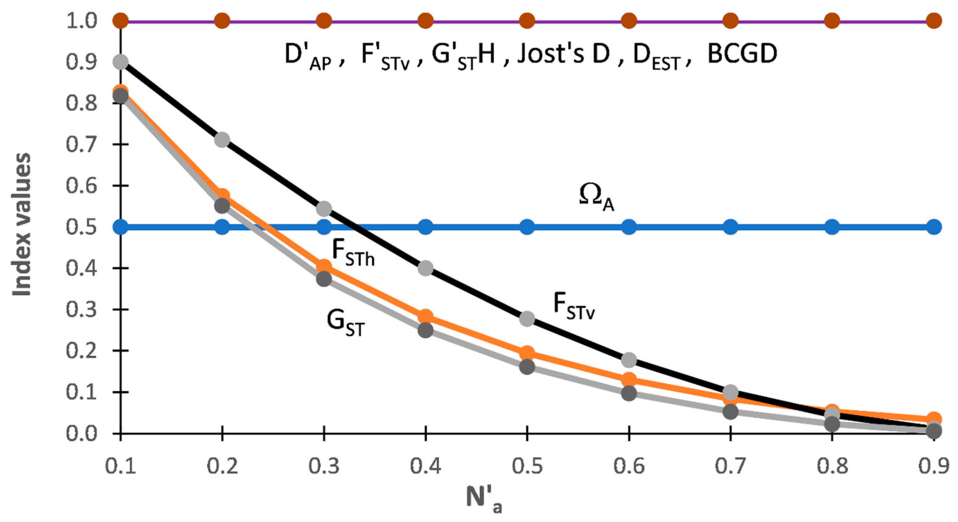
Figure 1 shows the outcome of the analyses for among population indices based on DS-I. One thing that clearly stands out is that ΩAP and FSTv are unequivocally measuring different aspects of population structure. ΩAP is constant at 50% of the N′a across the range of allelic diversity present within these subsets while FSTv ranges from 1.0 (near Na-MIN) to 0.0 (at/near Na-MAX). At the minimal allelic diversity (Na-MIN), when there is just one allele across both populations, ΩAP = 0 while FSTv is undefined (online Supplemental Table S1). The pattern for ΩAP (Figure 1) shows that it is a differentiation measure. Based on DS-I, ΩAP is independent of the level of DT when there is no allelic overlap among populations. In sharp contrast, FSTv has an inverse relationship with the level of N′a present in each subset, being highest at minimal levels of N’a and having a sigmodal decrease as N′a increases. At N′a-MAX, when every individual in a subset has unique alleles for a given marker, all pairwise comparisons are identical and net variance only occurs within individuals (online Supplemental Table S1). In other words, at N′a-MAX AMOVA is completely blind to the corresponding ΔAI and ΔAP that is present. This pattern indicates that FSTv is a fixation measure that tracks the relative degree of fixation in each population pair and that is strongly affected by the level of DT. In strong contrast, ΩAP shows that each population has half of the total allelic diversity present in each subset. Although measuring different things, ΩAP ≈ FSTv when N′a = 0.03 to 0.035 (Figure 1), indicating that the extent of differentiation (ΩAP) and degree of fixation (FSTv) have comparable values around this level of N′a with DS-I.
TDAP-Formatted Indices
By design F′STv and D′AP both = 1.0 across all subsets (Figure 1) and these two TDAP-formatted indices, consequently, fail to show that the two approaches are measuring different aspects of population structure with this data set.
Other among Population Indices
Results for the other ‘among population’ indices show that FSTh and GST both follow a pattern across the nine subsets similar to that shown by FSTv (=G′STN) (Figure 1). This indicates that, similar to FSTv, the heterozygosity-based MTAP-formatted indices are also tracking the fixation present among populations. As with D′AP and F′STv (=G″ST), the four other TDAP indices (G′STH, Jost’s D, DEST, and BCGD) all equal ‘1.0’ across the nine subsets with this data set.
3.1.2. Among Individuals within Populations (ΩAI and FAI)
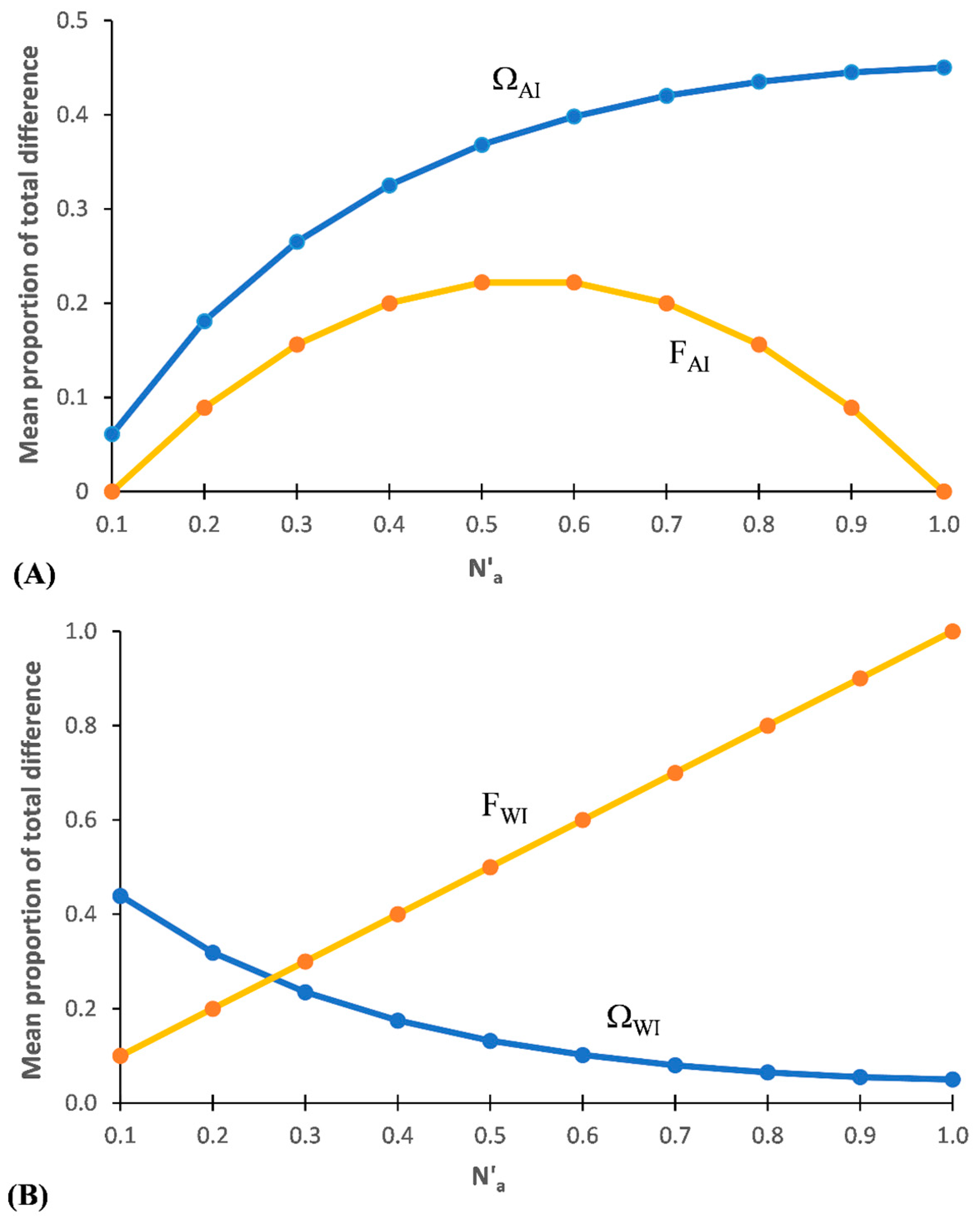
The percentage of total DT and FT represented among individuals nested within populations (ΩAI and FAI, respectively) across the maximum range of Na possible with these subsets is shown in Figure 2A. FAI shows a pattern similar to that of an optimum response curve, with FAI = 0.0 at/near Na min and also at/near Na-MAX and peaking at FAI ≈ 0.22 in subsets around N′a ≈ 0.55%. At low values for N′a in a subset, both variance among individuals (FAI) and that within individuals (FWI) rise (Figure 2B) as N′a increases. However, as N′a continues to increase, a point is reached where a large percentage of the combinations of the different alleles present results in the maximum value for the basal stratum (FWI). This saturation redundancy for FWI is one reason why AMOVA is blind to allelic diversity. Further increases in N′a will lead to both increasing levels of saturation redundancy and also to decreasing levels of variance among all individuals (FIT) until the only net variance remaining is that within individuals (occurring when DT = N′a-MAX).
The pattern for ΩAI indicates that it measures differentiation among individuals, with ΩAI increasing as DT increases, reaching a peak at N′a = 1. Thus, every allele is counted and the problem of saturation redundancy associated with AMOVA is lacking with SIDTA. ΩAI exceeds the corresponding FAI value across the subsets, with the divergence between the two measurements increasing notably at very high levels of DT. When ΩAI is maximal with DS-I (at N′a = 1.0) the corresponding value is FAI = 0.0 (Supplemental Table S1).
3.1.3. Within Individuals (ΩWI and FWI)
With diploid data, the proportion of total variance found within individuals (‘FWI’) increases as N′a increases, with ‘FWI’ = 1.0 at N′a = 1.0 (=Na-MAX) for these data sets (Figure 2B). This pattern suggests that FWI is tracking the extent of fixation, but in the opposite direction that is measured by FSTv. In contrast, the proportion of DT found within individuals (ΩWI) follows a curvilinear decrease with increasing N′a, with ΩWI = 1.0 at the theoretical minimum N′a and decreasing τo ΩWI = 0.05 at the maximum (N′a = 1) with these data sets (Supplemental Table S1).
3.2. Analyses of Data Set II
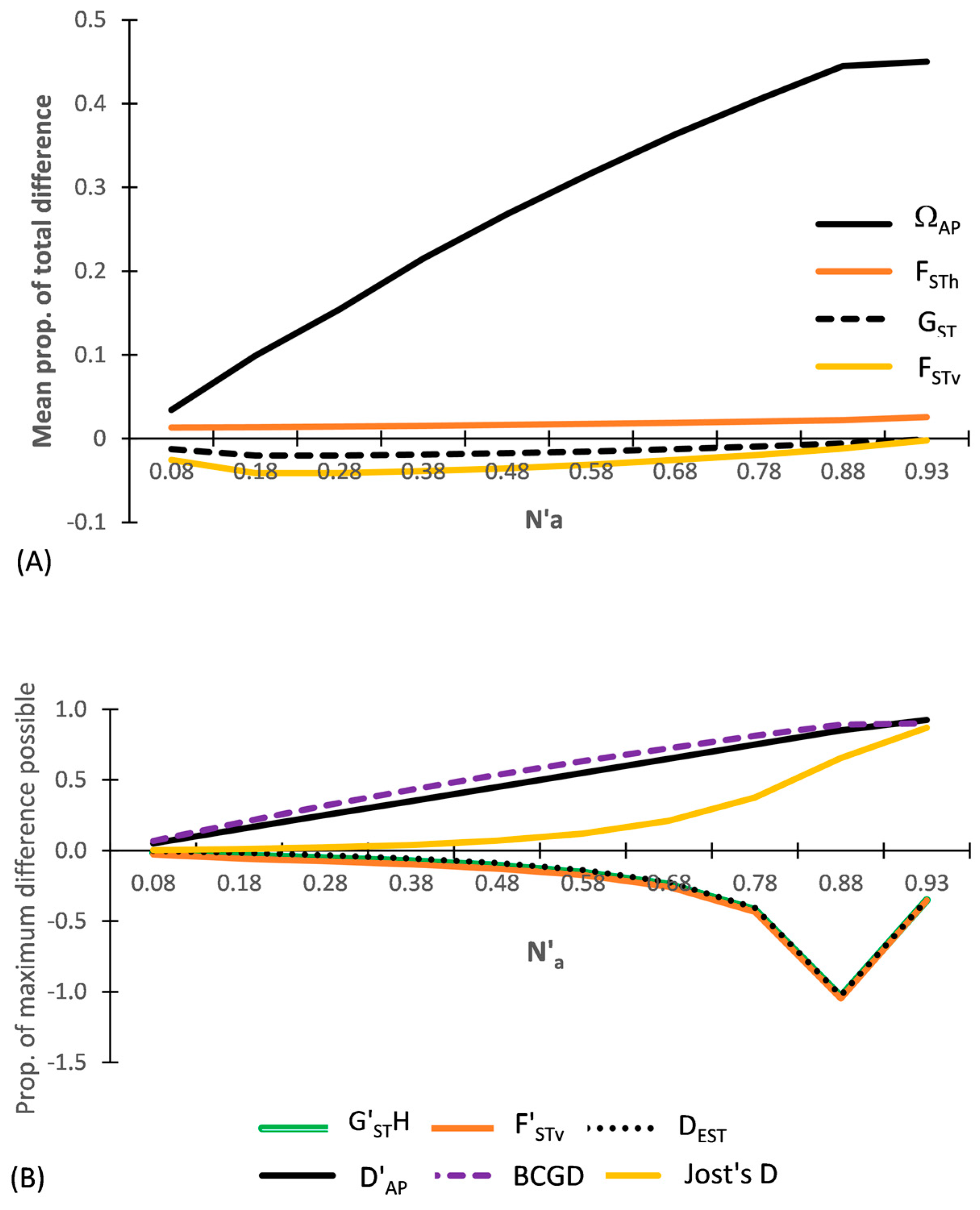
The results for DS-II are shown in Figure 3, which focuses only on among population indices. By having the level of heterozygosity and variance balanced between each population pair, the differentiation between each population pair is minimal. Thus FSTh, FSTv, and GST are minimal (close to ‘0’) across all subsets. A distinct demarcation exists between the three entropic based diversity indices (ΩAP, D′AP, DAP (not shown) and also by BCGD, which are all positive while, with the exception of FSTh and Jost’s D, all of the other heterozygosity and variance-based indices (FSTv, GST, G′STH, F′STv, and DEST) are all negative (Figure 3). The presence of positive and negative values among the various heterozygosity-based indices for the same subset is addressed in Section 4.
3.2.1. MDAP Indices
ΩAP closely tracks changes in N′a, being half of D′AP and positive across all subsets (Figure 3A). In contrast, FSTv is negative and very close to ‘0.0’ across all subsets, differing greatly from ΩAP. Divergence between these two indices increases notably as N′a approaches N′a-MAX. The heterozygosity-based MDAP indices closely follow the same pattern as that shown by FSTv, with all values tracking very close to 0.0 across all subsets. However, the unadjusted FSTh is positive across all subsets while the adjusted heterozygosity MDAP indices (GST and G′STN (=FSTv)) are slightly negative across all subsets. These patterns clearly show the difference between what the fixation indices (FSTv (=G′STN), FSTh, GST) measure and what is measured by ΩAP, which is a differentiation measure.
3.2.2. TDAP Indices
By design, the TDAP indices vary across the subsets with DS-II (Figure 3B). D′AP is twice as large as ΩAP (Figure 3A) and closely tracks changes in allelic diversity as N′a increases across the subsets. In striking contrast to the results of DS-I, D′AP differs notably from all of the TDAP-formatted heterozygosity- and variance-based indices (Figure 3B). Jost’s D stands out from the adjusted heterozygosity-based TDAP indices in being positive across all subsets of DS-II, showing a sigmoidal increase as N′a increases, with a prolonged slow rate of increase across subsets having a low N′a (Figure 3B). Notably, this sigmodal response, which is typical of q = 2-based diversity indices, lies well below the corresponding D′AP and BCGD values for all of the subsets, except near the two end points. It even falls below ΩAP up until N′a = 0.78. F′STv is negative and becomes more negative as N’a increases across the subsets. G′STH, G″ST, and DEST diverge from the pattern shown by Jost’s D as N′a increases across the subsets and instead closely track F′STv, with (G″ST = F′STv). BCGD closely tracks the level of N′a across the nine subsets, yielding values very close to those of D′AP. Linear regression shows that of the TDAP indices, BCGD has the tightest fit with N′a (y = x − 0.0025; R2 = 1.0; p < 0.001), with D′AP falling very close behind (y = 1.0245x + 0.0256; R2 = 0.9938; p < 0.001).
3.3. Analyses of Data Set III
3.3.1. MDAP-Formatted Indices
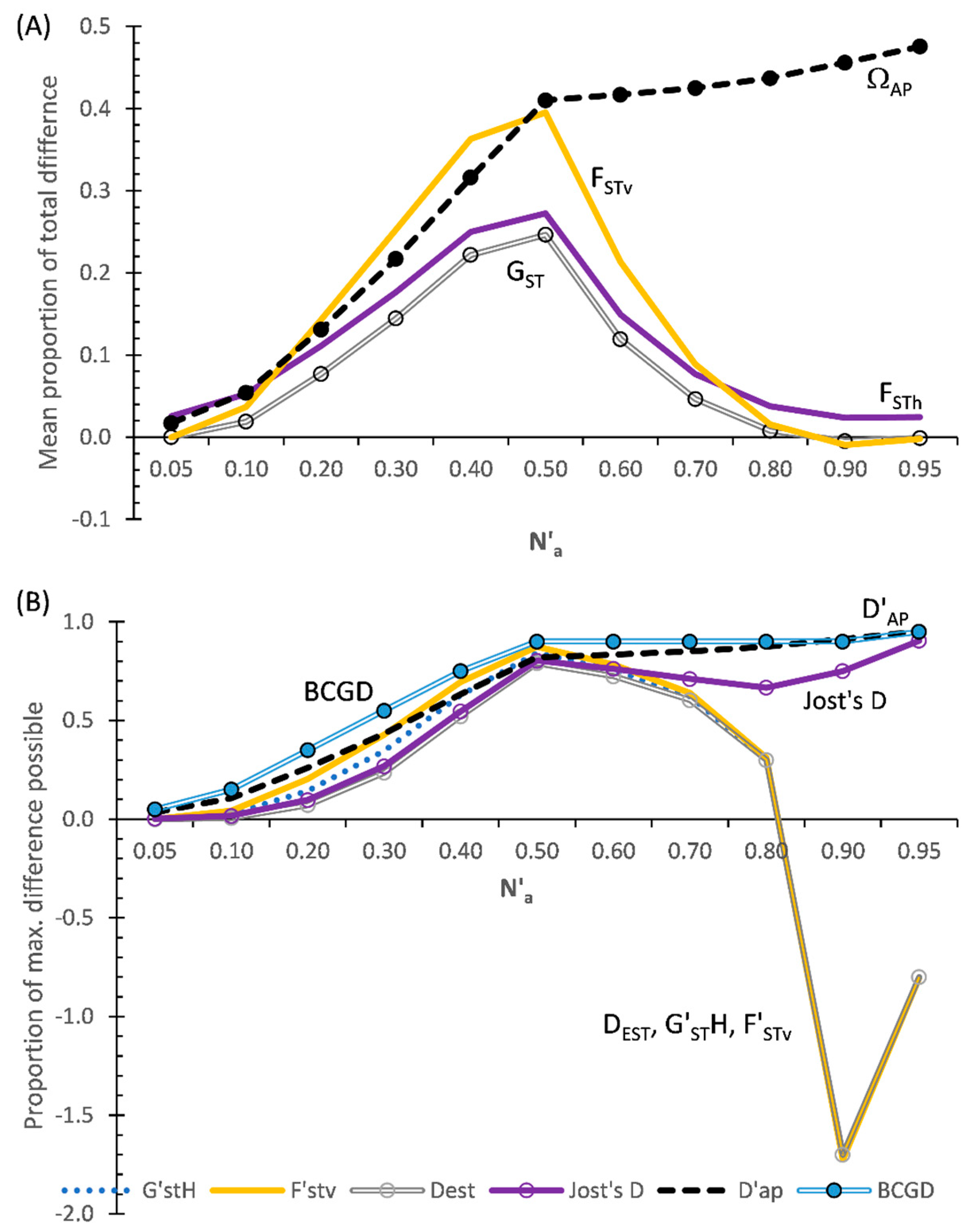
Figure 4A shows the results for the MDAP-based indices based on Data Set III. What stands out in this figure is that although ΩAP increases as N′a increases across all subsets of DS-III, FSTv at first increases as N′a increases and it then decreases abruptly above N′a = 0.5. The three MDAP heterozygosity-based indices (FSTh, GST, and G′STN) follow a similar pattern, or an identical pattern in the case of G′STN, to that of FSTv. As seen with DS-II (Figure 3A), the adjusted GST closely tracks FSTh across all subsets (Figure 4A). In comparison with the heterozygosity-based values (except for G′STN), FStv more closely compares to ΩAP between N′a = 0.2–0.5 with this data set than either FSTh and GST do. Both FSTv and GST become slightly negative above N′a = 0.8, while FSTh remains positive across all subsets. This pattern conforms with the information in Supplemental Table S2.
3.3.2. TDAP-Formatted Indices
As found with DS-II, D′AP differs notably from all of the TDAP-formatted heterozygosity and variance-based indices with DS-III (Figure 4B). D′AP increases as N′a increases across all subsets. Although comparable to D′AP across all subsets, the TDAP-formatted BCGD flatlines (at BCGD = 0.9) across subsets N′a = 0.5–0.9. In contrast, F′STv and the heterozygosity-based indices all show both increases and decreases across the subsets of DS-III (Figure 4B), with FSTh always being positive while FSTv and the adjusted heterozygosity-based indices are both positive and negative.
All of the TDAP indices coincide around N′a = 0.5, occurring due to one population having very low diversity (e.g., high homozygosity) at that point, while the second population has a very high allelic diversity (high heterozygosity). F′STv most closely matches D′AP up to N′a = 0.5 and then greatly deviates from that index. After closely tracking Jost’s D up to N′a = 0.5, the adjusted heterozygosity indices (DEST G′STH, and G″ST) above that point all greatly diverge from Jost’s D and instead closely track F′STv (Figure 4B).
3.4. Analyses of Natural Populations
The patterns of genetic structure associated with the three data sets using ‘artificial’ populations are unique to those data sets. Although differing from the patterns associated with the artificial populations in some respects, analyses of the natural population data sets all show ΩWI decreasing with increases in N’a.
3.4.1. Monomorphic Markers
To study the influence of monomorphic markers on SIDTA and AMOVA, analysis of STAB subsets of haploid data was undertaken (Supplemental File S2). One set of ten STAB SSRs (STAB-10) included two monomorphic SSRs. The second set (STAB-8) had the same SSRs excluding the monomorphic SSR-16 and SSR-19. Because AMOVA sums variance across markers, monomorphic markers, for which variance = 0, do not affect FST. Consequently, FST is identical with both the STAB-8 and STAB-10 sets (FST = 0.53). In contrast, ΩAP = 0.26 based on the STAB-8 set and ΩAP = 0.21 with the STAB-10 set. This difference results from two things: (1) monomorphic markers have a diversity value of 1.0, and (2) SIDTA averages the diversity across markers. Consequently, the presence of monomorphic markers in a data set has the potential to reduce ΩAP. The larger the proportion of monomorphic markers included in a data set the greater the potential reduction. However, the inclusion of monomorphic markers in a data set allows for that level of diversity to be counted in studies on genetic structure. With the exception of the STAB-10 set used here and the data set showing theoretical minimum allelic diversity (where there is just one allele present), all of the data sets used in this study lack monomorphic SSRs to allow for a more direct comparison of SIDTA and AMOVA.
3.4.2. Haploid Data Set
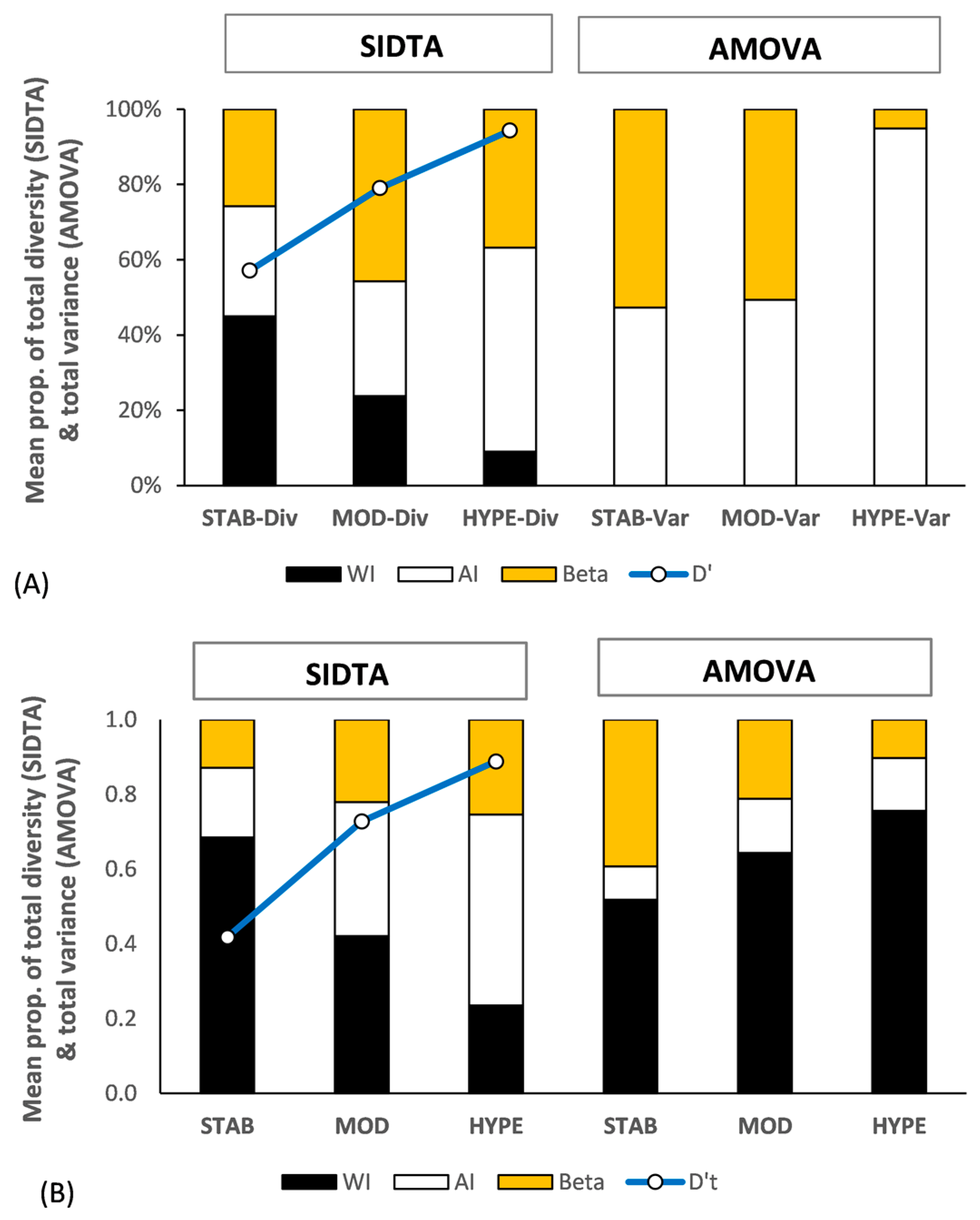
Figure 5A shows the genetic structure across the three data sets for the haploid gametophytes of Sphagnum comosum Müll. Hal. and of S. novo-zelandicum Mitt. (14 samples each). The relationship between ΩAP and FSTv basically conforms with the pattern seen in Figure 1, with (ΩAP ≪ FSTv) at lower N′a values, (ΩAP ≈ FSTv) at moderate N′a values, and (ΩAP ≫ FSTv) at very high N′a values. The extent of fixation between populations (FSTv) greatly exceeds the differentiation between populations (ΩAP) with the STAB subset, with the reverse being the case with the HYPE set. D′T for the three data sets is 0.49 for the STAB subset, 0.79 for the MOD subset, and 0.94 for the HYPE subset. Both ΩAP and FSTv are significant across all three data sets (α = 0.05) with p values for ΩAP being more significant with the MOD and HYPE subsets than the corresponding p values for FSTv.
As there is typically no variance within haploid individuals, all variance is among individuals with AMOVA at that ploidy level. In contrast, ΩWI = 1 with haploid data, and this allows for allelic diversity to occur both within and among individuals. This increases the difference between FSTv and ΩAP values with haploid data, particularly at lower levels of N′a. However, as ΩWI = 1 across the STAB, MOD, and HYPE subsets, this difference is largely offset by the higher levels of N′a associated with the MOD and HYPE subsets (Figure 5A).
3.4.3. Diploid Data Set
Figure 5B shows the genetic structure of two artificial diploid populations of Sphagnum novo-zelandicum (six samples each) based on both SIDTA and AMOVA across the three SSRsub sets. With diploid data, both SIDTA and AMOVA have the potential for a within individual stratum. The diploid data follow the same general pattern present in the haploid data, with the exception of the inclusion of the ‘within individual’ stratum with AMOVA. There is an increase in ΩAP and a corresponding decrease in FSTv as N′a increases, with ΩWI and FWI following the opposite pattern along that gradient. As with the haploid data, (ΩAP ≪ FSTv) at lower N′a values, (ΩAP ≈ FSTv) at moderate N′a values, and (ΩAP > FSTv) at very high N′a values. The diploid SIDTA data differs from the haploid data in that ΩWI is higher and ΩAP is lower than that for the haploid data across the three data sets. The increase in ΩAIT as N’a increases mostly occurs in ΩAI, while the decrease in FIT as N’a increases lies in FSTv. The diploid AMOVA data shows that the majority of variance within populations occurs within individuals with this data set. Both ΩST and FSTv are significant (α = 0.05) for the STAB and MOD subsets but differ with the HYPE subset, with the p value being not significant for ΩAP (p = 0.206) and significant with the corresponding p value for FST (p = 0.014).
3.4.4. Allopolyploid Data Sets
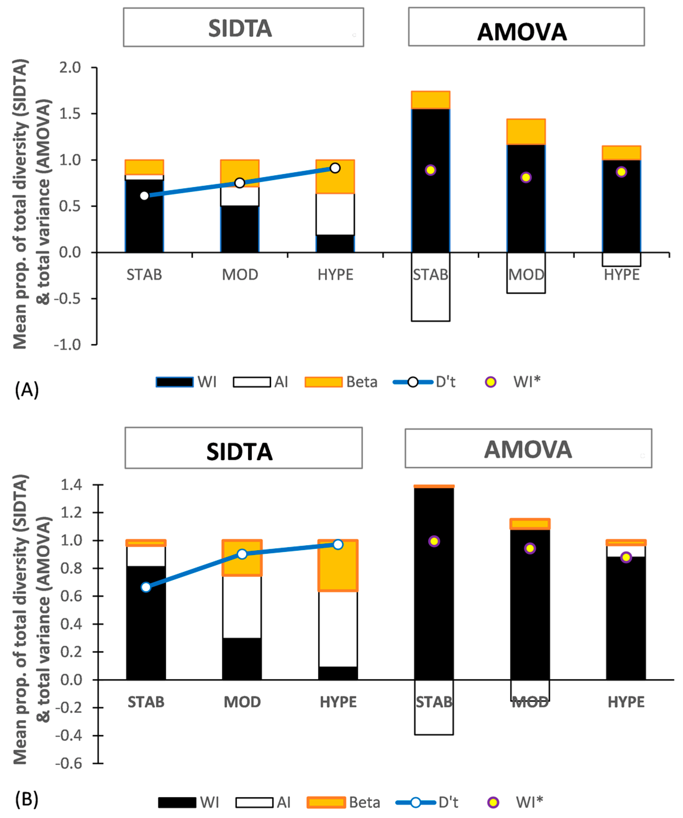
Figure 6 shows the population structure based on SIDTA and AMOVA across three SSR subsets for gametophytic populations of allopolyploid Sphagnum species. Figure 6A is based on regional populations of two gametophytically allodiploid Sphagnum species: the Hawaiian population of S. × palustre L. and the South Island, NZ population of S. ×cristatum Hampe, each with 31 samples. Figure 6B is based on two South Island, New Zealand populations of the gamtetophytically allotriploid Sphagnum × falcatulum Besch., each with f21 samples. AMOVA yields negative FAI values for both allopolyploid data sets, resulting in complex and puzzling population structures. In strong contrast, lacking negative values, SIDTA shows that both the allopolyploids follow the same general pattern for population structure as seen for SIDTA applied to the non-allopolyploid data sets: with (1) ΩWI decreasing with increasing allelic diversity, and (2) ΩAP increasing along the same gradient (Figure 6).
Based on AMOVA, negative estimated variance among individuals nested within populations occurs and it is included in the calculation of FSTv, FAI, and FWI for both ploidy levels, resulting in negative FAI values. Negativity in FAI decreases as marker variability increases. While negative FAI values occur across all three SSR subsets with the allodiploid data, they are limited to the STAB and MOD SSR subsets with the allotriploid data (Figure 6A,B). The greatly distorted population structure that AMOVA sees in the presence of negative F values is evident in these figures. For instance, the presence of negative values results in FWI > 1.0. With AMOVA, negative FAI values arise when the mean square within individuals exceeds the mean square among individuals nested within populations. Finally, both the allodiploid and allotriploid data sets show FWI being highest with the STAB subset and declining as SSR variability increases, the opposite pattern of that seen in the non-allopolyploid data sets.
For comparison purposes, F statistics based on negative estimated variance among individuals nested within populations treated as 0.0 were also calculated and are indicated with an asterisk (e.g., FST*). The values for FWI* are indicated by yellow dots in Figure 5A,B, and they are all higher than the corresponding FWI seen with the STAB and MOD subsets with the diploid data (Figure 5B) and also at comparable N’a values in Figure 2B.
4. Discussion
AMOVA and SIDTA (Shannon informational diversity translation analysis) are shown to yield highly different assessments of the hierarchical genetic structure of populations, with all levels of the hierarchy being affected. Thus, using either diversity or variance to explore the genetic structure of populations is akin to studying a species using a visual assessment versus using one based on scent. Differences between the two approaches are most pronounced when markers are highly stable and also when hypervariable markers are employed. Furthermore, wrestling with negative among group variance values and F statistic values frequently arises in population studies based on AMOVA, particularly with allopolyploids. This problem is a non-issue with SIDTA, which lacks negative among group differentiation values.
AMOVA also yields the [<0, 1] MDAP-formatted PHiPT index (an estimate of ΦPT, an analogue of FSTv) [27]. PHiPT calculates population differentiation simply based on genotypic variance by suppressing variation within individuals. Thus, PhiPT is typically larger than FSTv (or more negative) and its behavior as N′a changes closely tracks that of FSTv. It was excluded from this study because it ignored variance within individuals. A similar [0, 1] index could be created for SIDTA:
ΨAP =ΔAP/(ΔAP + ΔAI)
Unlike the heterozygosity- and variance-based MDAP-formatted indices (e.g., FSTv, FSTh, GST, G′STN), which measure fixation, the MDAP-formatted ΩAP index yields an assessment of differentiation among populations based on allelic diversity. The addition of ΩAP provides SIDTA with MDAP-, TDAP-, and ENP-based indices. Additionally, the suite of MD-formatted differentiation indices (e.g., ΩAI, ΩAP, ΩAR, etc.) allows for SIDTA-based analyses of the hierarchical genetic structure of populations to be clearly and effectively presented, as shown in Figure 5 and Figure 6.
4.1. Formats of Measurement
In addition to distinguishing between indices that measure fixation from those measuring differentiation, it is also useful to group them by how they express this (e.g., focus on the mean difference among populations (MDAP) vs. focus on the total difference among populations (TDAP)). For instance, a recent paper notes that Jost’s D is often mistakenly used as an estimator of GST [1]. Such a misunderstanding would be less likely if, in addition to knowing that GST is a fixation index and Jost’s D is a differentiation index, it was also understood that the former has an MDAP format, and the latter has a TDAP format.
4.2. Effective Number of What?
It has been shown that expected homozygosity data can be translated into effective number of alleles [2,33]. Although both the q = 1-based SIDTA and the q = 2-based expected heterozygosity measures can be associated with effective numbers data, just what the effective numbers of alleles represents differs between the two approaches. The q = 1 effective number of alleles (exponential of Shannon entropy) is the number of equally common alleles needed to achieve the entropy of allele identity in the population. It is not tied to a given ploidy level and is also not focused on the extent of heterozygosity that is present. In contrast, the q = 2 effective number of alleles is the number of equally common alleles needed to achieve the expected heterozygosity of the alleles in a population of diploid organisms. Thus, D′AP and Jost’s D (and DEST) clearly measure different parameters. They only yield the same value when (1) two populations have identical alleles and allele frequencies (DEST = Jost’s D = D′AP = 0.0), and when (2) there are no shared alleles between two populations (DEST = Jost’s D = D′AP = 1.0). Between these two extremes, and based on DS-II and DS-III, D′AP is typically both greater than, and also tracks closer to N′a than either Jost’ D or DEST do (see Figure 3 and Figure 4B).
4.3. Comparison with Other among Population Indices
The only MDAP index to measure differentiation examined in this study is ΩAP. The other widely used heterozygosity-based and variance-based MDAP indices are all fixation measures. Based on this survey, ΩAP is the sole choice if one needs an assessment of mean differentiation among populations.
The TDAP indices examined in this study all measure allelic differentiation, but they differ in the parameters that they measure: D′AP tracks allelic diversity, the heterozygosity-based indices (G′STH, G″ST (=F′STv), Jost’s D, DEST) focus on the probability of alleles being in a heterozygous pairing, F′STv measures variance among genotypes. Not a part of the Hill-number family of diversity measures [21,34], BCGD measures allelic differentiation by comparing the similarity of simple allele frequencies (or relative allele frequency) between two populations. Although BCGD was found by [21] to have close a relationship to GST and FST, this study unequivocally shows that BCGD yields results close to those of the q = 1-based SIDTA D′AP and that they are highly divergent from those of the q = 2 indices (both expected heterozygosity based and variance based).
Although all of the TDAP-formatted indices are equal to 1.0 with DS-I, that is what they were designed to do at the maximum values of the respective parameters that they measure. However, there are striking differences among their overall respective performances in DS-II and DS-III (Figure 3 and Figure 4B). The most notable demarcation among the TDAP indices shows two primary subgroups, with D′AP and BCGD in one group (subclass I) and all of the q = 2 indices in a second grouping (F′STv (=G″ST), G′STH, Jost’s D, DEST) (subclass II). Subclass I indices track ‘q = 0’ far more closely than the ‘q = 2’ subclass indices do. This reflects how the subclass I indices are related to ‘q = 0’ diversity values, where each allele has the same weight (1). BCGD is based on simple allelic frequency (or relative allele frequency), which is related to q = 0 data (where each allele has equal weighting) by ‘1∙pi’, where pi is the relative frequency of an allele in a population. BCGD differs from the q = 1 SIDTA indices, which are related with q = 0 data by ‘1∙pi∙(ln pi)’. The SIDTA approach tends to dampen (i.e., make more equitable) the differences in frequency among the alleles in a population. Thus, these two subclasses I indices typically remain relatively close to q = 0 diversity data. Although BCGD closely tracks changes in allelic diversity among populations with DS-I and DS-II, it fails to always do so with DS-III. This indicates that BCGD does not track changes in allelic diversity in some cases. In contrast, the SIDTA-based D′AP closely tracks changes in allelic diversity across all three of the stress test data sets.
In contrast, the incorporation of q = 2 data with q = 0 data is achieved by ‘1∙pi2’, with the squaring of relative frequency data typically greatly increasing the difference between q = 0-based data and q = 2-based data, particularly when compared to that associated with the subclass I indices. Squaring the relative frequency of each allele results in more weight being given to alleles having high frequency and very little weight being given to uncommon alleles. This results in q = 2 indices measuring notably different parameters than those measured by the subclass I indices. The heterozygosity-based TDAP indices, which include Jost’s D, DEST, G′STH. and G″ST (=F′STv), are unequivocally shown to be tracking changes in the probability of expected heterozygosity by their performance in DS-II and DS-III. Another difference between the two subclasses is that subclass I indices are positive across the three stress test data sets while the adjusted heterozygosity-based indices and the variance-based indices of the subclass II have both positive and negative values.
The two unadjusted heterozygosity indices, FSTh and Jost’s D, which are restricted to lie within the interval from 0 to 1, are both positive across all three stress test data sets. In contrast, negative values occur in the ‘adjusted’ expected heterozygosity indices (MDAP: GST, G′STN (=FSTv); TDAP: G′STH, G″ST (=FSTv), DEST). The ‘adjusted’ expected heterozygosity indices are all positive in DS-1, all negative in DS-II, and both negative and positive with DS-III. The negative values result from the adjustments for small population size and inbreeding in the calculations made by GenAlEx for these indices. The adjustment leads to increases in both HS and HT relative to the corresponding unadjusted HS and HT values, but with HS being increased more than HT. The imbalance between the adjusted HS and HT values becomes greater with increases in N′a and negative values for estimated heterozygosity occur when HS > HT. With DS-II, this adjustment results in the adjusted estimated heterozygosity values always being negative. The occurrence of negative ‘among population’ values in the ‘adjusted’ heterozygosity indices closely tracks the occurrence of negative values in FSTv and F′STv. Consequently, one of the notable outcomes of ‘adjustment’ made by GenAlEx to several of the heterozygosity-based indices is that it allows for heterozygosity-based indices to more closely match the entire spectrum of FSTv and F’STv based values. Indeed, a bit of additional tweaking results in two heterozygosity-based indices being equivalent to variance-based indices (i.e., G′STN = FSTv and G″ST = F′STv).
4.4. Drawbacks to ‘q = 2’ Indices
Although it is not an issue for q = 1 differentiation measures, one drawback for q = 2-based differentiation measures is that an incremental change in allele number and frequency has a much smaller change on the resulting value of a given index when N′a is lower than when that same incremental change occurs when N′a is very high, given their sigmoidal nature. This is problematic for a differentiation measure to have. Another drawback to the q = 2 differentiation measures is that they were primarily designed for diploid genotypic data. Thus, their application to allopolyploids is problematic, especially with gametophytic data. For instance, negative variance values are considered as representing excess heterozygosity [35] and/or the absence of population structure [36]. However, homologous chromosomes are typically lacking in the gametophytes of allopolyploid plants having disomic inheritance. Thus, ‘true’ heterozygosity does not usually occur in the gametophytes of such allopolyploids. Differences among/between the component monoploid genomes of alloploid gametophytes, which is measured by the allelic diversity within individuals (ΔWI), represents the allelic differentiation (ΩWI) among/between the ancestral monoploid genomes, not heterozygosity [37]. In such cases, negative F statistics should unequivocally not be considered as having excessive heterozygosity. In terms of negative variance values reflecting a lack of population structure, the data presented here shows that, based on SIDTA, structure is often present in allopolyploid gametophytes when negative variance occurs based on AMOVA. In the absence of population structure, SIDTA would yield ‘0.0’, not a negative value.
4.5. Impact of Marker Variability
Marker variability has a major effect on the genetic structure of populations and the nature of this influence differs markedly when based on SIDTA versus AMOVA. Some of these effects are discussed in the section on negative F statistics below.
With both haploids and diploids, the proportion of total allelic diversity within individuals (ΩWI) decreases with increasing marker variability while the reverse is the case for the proportion of variance within individuals (FWI). This pattern also holds true for ΩWI in allopolyploids, and, in the absence of negative values, it is also true for FWI. However, the frequent occurrence of negative values with AMOVA-based F statistics both greatly confuse this pattern for allopolyploids, and, also, notably distort the genetic structure of a population. The negative values are often associated with, but not limited to, FAI (the proportion of total variance (FT) represented by variance among individuals within populations). The most negative values occur with highly stable markers and then decline with increasing marker variability and, in some cases negative F values may be lacking with hypervariable markers. In contrast, negative values are lacking altogether in SIDTA-based indices.
Careful consideration needs to be given to the variability of markers selected to study genetic structure as well as their influence on the method(s) of analysis used. In terms of marker variability, a strong focus on highly variable markers leads to a high degree of divergence among individuals within a stratum, and this has the potential to minimize, or completely mask, strong evolutionary signals that may be found in markers having lower variability [18,19,37]. In addition, the resulting high divergence among individuals within a stratum obtained by highly variable markers yields notably lower overall similarity among its members. As the level of divergence among its individuals increases, the cohesive nature of a species decreases.
4.6. Notes on Negative ‘F’ Statistics with AMOVA
Although lacking with SIDTA, negative F statistics are ‘part and parcel’ of AMOVA and are notably particularly an issue with allopolyploids. Negative values notably distort the interpretation of the genetic structure of a population, making interpretation difficult. They are often associated with, but not limited to, FAI. As noted above, the most negative ‘F’ values occur with highly stable markers and then decline with increasing marker variability. The following is a brief discussion about the negative ‘F’ statistics associated with allopolyploids.
Based on DS-I, FWI is directly closely tied to N′a (Figure 2A), with high values of FWI only occurring at correspondingly high values of N′a. This is not always the case, however, as can be seen with the allopolyploid data where, in addition to the HYPE SSRs, high values of FWI* are also associated with the STAB and MOD subsets (Figure 6). In allopolyploids having disomic inheritance, the difference among the component monoploid genomes typically result in a very high a mean diversity and variance within individuals (DWI), and these particular values are largely independent of marker variability. For instance, based on SIDTA, D′WI for the allodiploid data is (D′WI ≥ 0.97) across the STAB, MOD, and HYPE subsets, and that for allotriploid data is (D′WI ≥ 0.87). This implies that the corresponding estimated variance within each individual is close to maximum. Furthermore, negative estimated variance among individuals augments both FWI and FWI*. Both ΩAI and FAI in contrast, are highly affected by marker variability. In allopolyploids, markers having low to moderate variability (such as the STAB and MOD subsets) frequently yield mean square among individuals within populations values that are less than the corresponding high mean square within individual values with AMOVA, which results in negative FAI values. Markers having a sufficiently high variability (such as the HYPE subset) may yield mean square among individuals within populations values that exceed the high mean square within individual values, and thus provide positive FAI values in allopolyploids, as is the case for the allotriploid data (Figure 6B).
4.7. Influences of Ploidy Level
Ploidy level has two major influences in a comparison of AMOVA and SIDTA. One is at the haploid level, where there is allelic diversity within individuals (DWI = 1.0), while there is no variation among individuals (FWI = 0.0) with AMOVA. The second influence occurs primarily at diploid and higher ploidy levels where high divergence occurs among the respective component monoploid genomes. In such cases, AMOVA and the foundationally adjusted heterozygosity measures often yield negative values. Negative among group F values can occur with haploid data, but they occur more frequently at higher ploidy values, particularly with allopolyploids. Although this aspect is primarily a result of the extent of divergence among the component monoploid genomes, it is also influenced by ploidy level.
4.8. Interpreting FST Data from Prior Studies
Studies misinterpreting FST (both FSTv and FSTh) and GST as measuring differentiation have the major problem that their conclusions unequivocally do not measure differentiation. Based on marker variability one can gain some general information to partially mitigate this issue. Generally, but not always, highly stable markers are likely to have FST and GST values exceeding the corresponding allelic differentiation between/among populations (ΩAP). When highly variable markers are used, there is a high probability that the FST values are much lower than corresponding ΩAP values. Additionally, when moderately stable markers are used it is possible that their associated FST values may be somewhat comparable to ΩAP, despite measuring different things. The above is based on haploid and diploid ploidy levels. This pattern does not always apply to allopolyploids, where the frequent occurrence of negative F values, particularly FAI, distorts the interpretation of population structure.
4.9. Possible Issue with Adjustments Made for Small Population Size and Inbreeding
For both the fixation and differentiation heterozygosity-based indices, adjustments for the almost unbiased estimators of heterozygosity [28] and for inbreeding [29] result in the adjusted heterozygosity-based indices (1) typically being smaller than the corresponding unadjusted values (e.g., Jost’s D > DEST), and (2) yielding both positive to negative values while the unadjusted heterozygosity-based indices are always positive. However, the adjustments affect these fixation and differentiation indices differently. All three of the stress test data sets show the adjusted heterozygosity-based fixation indices (GST, G′STN) to closely follow FSTh across all subsets. In contrast, the heterozygosity-based differentiation indices show a more variable pattern. This is most clearly shown in Figure 4B, where positive DEST (as well as G″ST and G′STH) values closely track Jost’s D when N′a ≤ 0.5, but they greatly diverge from Jost’s D when N′a > 0.5, and ultimately become highly negative. These findings indicate that corrections, such as almost unbiased estimators, that are designed for fixation indices are problematic when applied to differentiation indices, particularly at high levels of allelic diversity. Given that the differentiation and fixation indices greatly differ in what they measure, it is not surprising that this is the case. Exploring why such adjustments result in such a complex relationship between Jost’s D and the adjusted heterozygosity-based differentiation indices (DEST, G″ST and G′STH) is beyond the scope of this study.
4.10. Final Thoughts
As the various allelic differentiation indices measure notably different parameters, it is clear that one size does not fit all. Thus, it is important to select the index (or indices) that match the focus of research being undertaken. If heterozygosity or variance are important causal variables in the given application, then heterozygosity-based q = 2 differentiation measures (e.g., Jost’s D, DEST, F′ST) should be used [15]. If alleles should be weighed by their population share, then q = 1 differentiation measures (e.g., D′AP, ΩAP) would be the clear choice. Finally, if the presence or absence of alleles is what matters, then a q = 0 differentiation measure should be used. In addition, there are other aspects to consider, including: (1) when the focus is on the hierarchical genetic structure of populations and not simply on differentiation among populations; (2) avoidance of the problem of negative values; (3) when studying allopolyploids. For these issues, the q = 1-based SIDTA suite of indices clearly fits the bill.
Because the subclass II (q = 2) differentiation measures (1) can decline with increases in allelic diversity and (2) can be negative, they unequivocally have limitations in the measurement of differentiation. Given this, studies focused primarily on how different two or more groups (e.g., populations, sub-species, species, etc.) are would most likely be best served by subclass I differentiation measures (e.g., BCGD, SIDTA). This is especially true when comparing groups above the population level, where allelic diversity likely plays a bigger role than either heterozygosity or variance do.
Supplementary Materials
The following supporting information can be downloaded at: https://www.mdpi.com/article/10.3390/e25030492/s1. Supplemental File S1: Artificial data sets. Supplemental File S2: Natural data sets. Table S1. Theoretical maximum and minimum values for allelic diversity and variance. Table S2. Range of values and expected behavior of the statistics used in this paper
Funding
This research received no external funding.
Institutional Review Board Statement
Not applicable.
Data Availability Statement
The data sets used in this study can be found in Supplemental Files S1 and S2 of this paper.
Acknowledgments
I thank the three anonymous reviewers and the academic editor for their informative and helpful comments and suggestions.
Conflicts of Interest
The author declares no conflict of interest.
References
- Jost, L.; Archer, F.; Flanagan, S.; Gaggiottii, O.; Hoban, S.; Latch, E. Differentiation measures for conservation genetics. Evol. Appl. 2018, 11, 1139–1148. [Google Scholar] [CrossRef] [PubMed] [Green Version]
- Jost, L. GST and its relatives do not measure differentiation. Mol. Ecol. 2008, 17, 4015–4026. [Google Scholar] [CrossRef] [PubMed]
- Jost, L. Partitioning diversity into independent alpha and beta components. Ecology 2007, 88, 2427–2439. [Google Scholar] [CrossRef] [Green Version]
- Jost, L.; DeVries, P.; Walla, T.; Greeney, H.; Chao, A.; Ricotta, C. Partitioning diversity for conservation analyses. Divers. Distrib. 2010, 16, 65–76. [Google Scholar] [CrossRef]
- Sherwin, W.B.; Jabot, F.; Rush, R.; Rossetto, M. Measurement of biological information with applications from genes to landscapes. Mol. Ecol. 2006, 15, 2857–2869. [Google Scholar] [CrossRef]
- Sherwin, W.B.; Chao, A.; Jost, L.; Smouse, P.E. Information theory widens the spectrum of molecular evolution and ecology. Trends Ecol. Evol. 2017, 32, 948–963. [Google Scholar] [CrossRef]
- Sherwin, W.B. Entropy and information approaches to genetic diversity and its expression: Genomic geography. Entropy 2010, 12, 1765–1798. [Google Scholar] [CrossRef] [Green Version]
- Smouse, P.E.; Whitehead, M.R.; Peakall, R. An informational diversity analysis framework, illustrated with sexually deceptive orchids in early stages of speciation. Mol. Ecol. Resour. 2015, 15, 1375–1384. [Google Scholar] [CrossRef]
- Chao, A.; Jost, L.; Hseih, T.C.; Ma, K.H.; Sherwin, B.; Rollins, L.A. Expected Shannon entropy and Shannon differentiation between subpopulations for neutral genes under the finite island model. PLoS ONE 2015, 11, e0125471. [Google Scholar] [CrossRef] [Green Version]
- Gaggiotti, O.E.; Chao, A.; Peres-Neto, P.; Chiu, C.-H.; Edwards, C.; Fortin, M.-J.; Jost, L.; Richards, C.M.; Selkoe, K.A. Diversity from genes to ecosystems: A unifying framework to study variation across biological metrics and scales. Evol. Appl. 2018, 11, 1176–1193. [Google Scholar] [CrossRef] [Green Version]
- Verity, R.; Nichols, R.A. What is genetic differentiation, and how should we measure it—GST, D, neither or both? Mol. Ecol. 2014, 23, 4216–4225. [Google Scholar] [CrossRef] [PubMed]
- Heller, R.; Siegismund, H.R. Relationship between three measures of genetic differentiation GST, DEST and G′ST: How wrong have we been? Mol. Ecol. 2009, 18, 2080–2083. [Google Scholar] [CrossRef]
- Gerlach, G.; Jueterbock, A.; Kraemer, P.; Deppermann, J.; Harmand, P. Calculations of population differentiation based on GST and D: Forget GST but not all of statistics! Mol. Ecol. 2010, 19, 3845–3852. [Google Scholar] [CrossRef] [PubMed]
- Leng, L.; Zhang, D.E. Measuring population differentiation using GST or D? A simulation study with microsatellite DNA markers under a finite island model and nonequilibrium conditions. Mol. Ecol. 2011, 20, 2494–2509. [Google Scholar] [CrossRef]
- Meirmans, P.G.; Hedrick, P.W. Assessing population structure: FST and related measures. Mol. Ecol. Resour. 2011, 11, 5–18. [Google Scholar] [CrossRef]
- Whitlock, M.C. G′ST and D do not replace FST. Mol. Ecol. 2011, 20, 1083–1091. [Google Scholar] [CrossRef]
- Excoffier, L.; Smouse, P.E.; Quattro, J.M. Analysis of molecular variance inferred from metric distances among DNA haplotypes: Application to human mitochondrial DNA restriction data. Genetics 1992, 131, 479–491. [Google Scholar] [CrossRef]
- Karlin, E.F.; Smouse, P.E. Holantarctic diversity varies widely among genetic loci within the gametophytically allotriploid peat moss Sphagnum × falcatulum. Am. J. Bot. 2019, 106, 137–144. [Google Scholar] [CrossRef]
- Karlin, E.F.; Robinson, S.C.; Smouse, P.E. Genetic diversity within and across gametophytic ploidy levels in a Sphagnum cryptic species complex. Aust. J. Bot. 2020, 68, 49–62. [Google Scholar] [CrossRef]
- Berner, D. Allele Frequency Difference AFD—An Intuitive Alternative to FST for Quantifying Genetic Population Differentiation. Genes 2019, 10, 308. [Google Scholar] [CrossRef] [PubMed] [Green Version]
- Sherwin, W.B. Bray-Curtis (AFD) Differentiation in Molecular Ecology: Forecasting, an Adjustment (AA), and Comparative Performance in Selection Detection. Ecol. Evol. 2022, 12, e9176. [Google Scholar] [CrossRef]
- Karlin, E.F.; Boles, S.B.; Shaw, A.J. Resolving boundaries between species in Sphagnum section Subsecunda using microsatellite markers. Taxon 2008, 57, 1189–1200. [Google Scholar] [CrossRef]
- Karlin, E.F.; Boles, S.B.; Shaw, A.J. Systematics of Sphagnum section Sphagnum in New Zealand: A microsatellite-based analysis. N. Z. J. Bot. 2008, 46, 105–118. [Google Scholar] [CrossRef] [Green Version]
- Karlin, E.F.; Hotchkiss, S.C.; Boles, S.B.; Stenøien, H.K.; Hassel, K.; Flatberg, K.I.; Shaw, A.J. High genetic diversity in a remote island population system: Sans sex. New Phytol. 2012, 193, 1088–1097. [Google Scholar] [CrossRef] [PubMed]
- Peakall, R.; Smouse, P.E. GENALEX 6: Genetic analysis in Excel. Population genetic software for teaching and research. Mol. Ecol. Notes 2006, 6, 288–295. [Google Scholar] [CrossRef]
- Peakall, R.; Smouse, P.E. GenAlEx 6.5: Genetic analysis in Excel. Population genetic software for teaching and research-an update. Bioinformatics 2012, 28, 2537–2539. [Google Scholar] [CrossRef] [PubMed] [Green Version]
- Peakall, R.; Smouse, P.E. Appendix 1–Methods and Statistics in GenAlEx 6.5; Australian National University: Canberra, Australia, 2015. [Google Scholar]
- Nei, M.; Chesser, R. Estimation of fixation indices and gene diversities. Ann. Hum. Genet. 1983, 47, 253–259. [Google Scholar] [CrossRef] [PubMed]
- Nei, M. Molecular Evolutionary Genetics; Columbia University Press: New York, NY, USA, 1987. [Google Scholar]
- Bray, J.R.; Curtis, J.T. An ordination of the upland forest communities of southern Wisconsin. Ecol. Monogr. 1957, 4, 325–349. [Google Scholar] [CrossRef]
- Shriver, M.D.; Smith, M.W.; Jin, L.; Marcini, A.; Akey, J.M.; Deka, R.; Ferrell, R.E. Ethnic affliation estimation by use of population-specific DNA markers. Am. J. Hum. Genet. 1997, 60, 957–964. [Google Scholar]
- Whittaker, R.H. Communities and Ecosystems, 2nd ed.; MacMillan Publishers: New York, NY, USA, 1975; p. 118. [Google Scholar]
- Kimura, M.; Crow, J. The number of alleles that can be maintained in a finite population. Genetics 1964, 49, 725–738. [Google Scholar] [CrossRef]
- Hill, M.O. Diversity and evenness: A unifying notation and its consequences. Ecology 1973, 54, 427–432. [Google Scholar] [CrossRef] [Green Version]
- Holsinger, K.E.; Weir, B.S. Genetics in geographically structured populations: Defining, estimating and interpreting FST. Nat. Rev. Genet. 2009, 10, 639–650. [Google Scholar] [CrossRef] [PubMed] [Green Version]
- Meirmans, P.G. Using the AMOVA framework to estimate a standardized genetic differentiation measure. Evolution 2006, 60, 2399–2402. [Google Scholar] [CrossRef] [PubMed]
- Karlin, E.F.; Smouse, P.E. Allo-allo-triploid SphagnumB × falcatulum: Single individuals contain most of the Holantarctic diversity for ancestrally indicative markers. Ann. Bot. 2017, 120, 221–231. [Google Scholar] [CrossRef] [Green Version]
Figure 1.
Results of five MDAP and seven TDAP indices based on SIDTA, AMOVA, and heterozygosity measures across a wide range of N′a for the nine pairs of artificial populations (subsets) of Data Set I (DS-I). Values for the MADP indices (ΩAP, FSTv (=G′STN), FSTh, GST) measure the mean proportion of total difference between two populations and the values for the TDAP indices (D′AP, F′STv (=G″ST), G′STH, Jost’s D, DEST, BCGD) measure the proportion of the theoretical maximum difference between two populations. The MDAP-formatted ΩAP measures both.

Figure 2.
Mean proportion of total allelic diversity and total variance represented based on Data Set I. (A) among individuals within populations (ΩAI and FAI, respectively), and (B) within individuals (ΩWI and FWI, respectively) between ten pairs of ‘artificial’ diploid populations across a wide range of N′a.

Figure 3.
Results of five MDAP and seven TDAP indices based on SIDTA, AMOVA, and heterozygosity measures across a wide range of N′a for the ten pairs of artificial populations (subsets) of Data Set II (DS-II). (A) Values for the MADP indices with (FSTv = G′STN) and (B) values for the TDAP indices (with F′STv = G″ST). The MDAP-formatted ΩAP represents both the mean proportion of total difference between two populations and the mean maximum difference possible between two populations. G′STH lies between F’STv and DEST and is barely visible.

Figure 4.
Results of five MDAP and seven TDAP indices based on SIDTA, AMOVA, and heterozygosity across a wide range of N′a across 11 pairs of artificial populations based on Data Set III (DS-III): (A) MDAP indices (with G′STN = FSTv) and (B) TDAP indices (with G″ST = F′STv). The MDAP-formatted ΩAP represents both the mean proportion of total difference between two populations and the mean maximum difference possible between two populations.

Figure 5.
Population genetic structure (black: within individuals; no fill: among individuals within populations; orange: between populations) yielded by SIDTA and AMOVA and based on STAB, MOD, and HYPE SSR subsets for haploid and diploid populations. (A) between regional populations of haploid gametophytes of Sphagnum comosum and S. novo-zelandicum (14 samples each) and (B) between regional artificial populations of diploid sporophytes of S. novo-zelandicum (6 samples each). The [0, 1] scaled diversity (D′T) for the total allele metric diversity detected with each data set is shown by the blue line. Beta refers to both ΩAP and FSTv.

Figure 6.
Population genetic structure (black: within individuals; no fill: among individuals within populations; orange: between populations) yielded by SIDTA and AMOVA and based on STAB, MOD, and HYPE SSR sets for allodiploid and allotriploid data. (A) regional populations of two gametophytically allodiploid species (South Island, NZ population of Sphagnum × cristatum and Hawaiian population of S.× palustre) and (B) two South Island, NZ populations of the gametophytically allotriploid Sphagnum × falcatulum. The [0, 1] scaled diversity (D′) for the total allele metric diversity detected with each data set is shown by the blue line. Beta refers to both ΩAP and FSTv. WI* refers to FWI* which is calculated by ignoring negative FAI values (i.e., treating them as 0.0).

Table 1.
Hierarchical population structure based on SIDTA (adapted from [8]). (EFNA: effective number of alleles). The theoretical minimum DT (DT-MIN) occurs when just one allele is present across all populations, and the theoretical maximum DT (DT-MAX) occurs with no allelic overlap within and among all samples across all populations.
| Allelic Diversity within Strata (as Effective Number of Alleles) | Differentiation between Strata [Multiplicative] (as Effective Number of Groups) | |
|---|---|---|
| DT = (grand total EFNA) | DAR = (EFN regions within study) | |
| DAR = (DT/DWR) | (3) | |
| DWR = (mean EFNA within regions) | DAP = (EFN populations within regions) | |
| DAP = (DWR/DWP) | (4) | |
| DWP = (mean EFNA within populations) | DAI = (EFN individuals within populations) | |
| DAI = (DWP/DWI) | (5) | |
| DWI = (mean EFNA within individuals) | ||
Table 3.
Hierarchical population structure based on the mean allelic diversity (Δ) among groups expressed as a proportion (Ω) of the grand total allelic diversity (DT).
Table 3.
Hierarchical population structure based on the mean allelic diversity (Δ) among groups expressed as a proportion (Ω) of the grand total allelic diversity (DT).
| Mean [0, 5] Differentiation between Strata | |
|---|---|
| ΩAP: Mean [0–0.5] scaled proportion of DT represented by DAP | |
| ΩAP = ΔAP/DT | (12) |
| ΩAI: Mean [0–0.5] scaled proportion of DT represented by DAI | |
| ΩAI = ΔAI/DT | (13) |
| ΩAIT = Mean [0–0.5] scaled proportion of DT represented by D among all inds. | |
| ΩAIT = ΔAIT/DT | (14) |
| ΩAIP = Mean [0–0.5] scaled proportion of DWP represented by DAI | |
| ΩAIP = ΔAI/DWP | (15) |
Disclaimer/Publisher’s Note: The statements, opinions and data contained in all publications are solely those of the individual author(s) and contributor(s) and not of MDPI and/or the editor(s). MDPI and/or the editor(s) disclaim responsibility for any injury to people or property resulting from any ideas, methods, instructions or products referred to in the content. |
© 2023 by the author. Licensee MDPI, Basel, Switzerland. This article is an open access article distributed under the terms and conditions of the Creative Commons Attribution (CC BY) license (https://creativecommons.org/licenses/by/4.0/).
Share and Cite
MDPI and ACS Style
Karlin, E.F. A Comparison of Entropic Diversity and Variance in the Study of Population Structure. Entropy 2023, 25, 492. https://doi.org/10.3390/e25030492
AMA Style
Karlin EF. A Comparison of Entropic Diversity and Variance in the Study of Population Structure. Entropy. 2023; 25(3):492. https://doi.org/10.3390/e25030492
Chicago/Turabian StyleKarlin, Eric F. 2023. "A Comparison of Entropic Diversity and Variance in the Study of Population Structure" Entropy 25, no. 3: 492. https://doi.org/10.3390/e25030492
Note that from the first issue of 2016, this journal uses article numbers instead of page numbers. See further details here.