Traceability Analyses between Features and Assets in Software Product Lines

Abstract

In a Software Product Line (SPL), the central notion of implementability provides the requisite connection between specifications and their implementations, leading to the definition of products. While it appears to be a simple extension of the traceability relation between components and features, it involves several subtle issues that were overlooked in the existing literature. In this paper, we have introduced a precise and formal definition of implementability over a fairly expressive traceability relation. The consequent definition of products in the given SPL naturally entails a set of useful analysis problems that are either refinements of known problems or are completely novel. We also propose a new approach to solve these analysis problems by encoding them as Quantified Boolean Formulae (QBF) and solving them through Quantified Satisfiability (QSAT) solvers. QBF can represent more complex analysis operations, which cannot be represented by using propositional formulae. The methodology scales much better than the SAT-based solutions hinted in the literature and were demonstrated through a tool called SPLAnE (SPL Analysis Engine) on a large set of SPL models.

1. Introduction

Software Product Line Engineering (SPLE) is a software development paradigm supporting the joint design of closely-related software products in an efficient and cost-effective manner. The starting point of a Software Product Line (SPL) is the scope, which defines all of the possible features of the products in the SPL. The scope is said to define the problem space of the SPL, describing the expectations and objectives of the product line. The description is typically organized as a feature model [1] that expresses the variability of the SPL in terms of relations or constraints (exclusion, requires dependency) between the features and defines all of the possible products in the product line.

An important step in SPLE is the development of core assets, a collection of reusable artifacts. The core assets contains the components, and we use the term component to represent any artifacts that contribute to product development, like code, design, documents, test plan, hardware, etc. A component is an abstract concept of any assets used in products. The core assets define the solution space of the SPL and are developed to meet the expectations outlined in the problem space [2]. They are developed for systematic reuse across the different products in the SPL [3,4]. The variability in core assets across the components is represented by a component model. The components in a component model may also have exclusions and require dependency constraints, similarly to feature models.

Given the problem and solution spaces for an SPL, as defined by the scope and the core assets, the next important step is traceability, which involves relating the elements (features, core assets) at these two levels [2].

The focus of this work is formal modeling and analysis of traceability in an SPL. There are many relationships possible; one of the most useful and natural one is the implementability relation that associates each feature in the scope with a set of core assets that are required for implementing the feature(s) [5]. Beside implementability, many other notions have been defined, thanks to the integration of the variabilities of the problem space and the solution space in the proposed framework. For example, one could be interested in checking whether every product in the problem space has a correspondence in the solution space, i.e., every product represented in the feature model can be implemented using the existing assets considering the implementability relation. Another example is the property to check every asset of an SPL that needs to be maintained not only because it is involved in some implementations, but the asset is the only option.

Let us consider an example from the cloud computing domain. The company offers a service to rent computers on a cloud with different possible software configurations using Linux-based distributions. In the back-end, instead of providing physical machines, the company provides virtual machines with some software package installed on them. Thus, the configuration of machines can be generated on demand according to the needs of the users. In order to improve the speed of the creation of a new machine, there are pre-configured machines ready to launch.

In this example, the possible configurations offered to the users define the problem space. The set of available Linux packages implementing the features is the core assets. The pre-configured machines can be seen as another set of assets (limited, but available immediately).

The following are some examples of relevant analyses that could arise in this example:

• Check if at least one of the pre-configured machines covers the needs of a new user configuration.
• Check if at least one of the pre-configured machines realizes (exactly) the needs of a new user configuration.
• Check if there are dead packages, i.e., packages that cannot be in any of the virtual machines.

In the literature, formal modeling and analysis of variability at the feature model level have been studied extensively, and several efficient tools have been built to carry out the analyses [6,7]. The main idea behind all of these works is that the variability analysis can be reduced to constraints and variables modeling the feature level variability [2,8,9,10,11,12,13,14,15]. While there are several recent works on traceability, most of them have confined themselves to an informal treatment [16,17,18,19]. Some works have chosen a formal approach for representing the traceability and configuration of features [20].

In the past, most of the work [6,7] has encoded variability analysis operations in propositional formulae. There are various SAT solvers, like SAT4j [21], or MiniSAT [22], or PicoSAT [23], which can be used to check the satisfiability of a propositional formula. We propose a novel approach for modeling traceability and other notions relating features and core assets using the Quantified Boolean Formula (QBF). QBF is a generalization of SAT Boolean formulae in which the variables may be universally and existentially quantified. The Quantified Satisfiability (QSAT) solver is used to check the satisfiability of the QBF. In this work, we make use of the well-known QSAT solver, CirQit [24] and RAReQS-NN [25].

An early version of this work was published [26]. The proposed method has been implemented in a tool that is integrated with the FaMa framework [27]. This tool, called SPLAnE (SPL Analysis Engine) [28], can model feature models, core assets (component models) and a traceability relations. SPLAnE is a feasible solution for the automated analysis of feature models together with asset relations. We believe that this article opens the opportunity for new forms of analysis involving variability models, assets and traceability relations. The following summarizes the contributions of this paper:

• A simple and abstract set-theoretic formal semantics of SPL with variability and traceability constraints is proposed.
• A number of new analysis problems, useful for relating the features and core assets in an SPL, are described.
• Quantified Boolean Formulae (QBFs) are proposed as a natural and efficient way of modeling these problems. The evidence of the scalability of QSAT for the analysis problems in large SPLs (compared to SAT) is also provided.
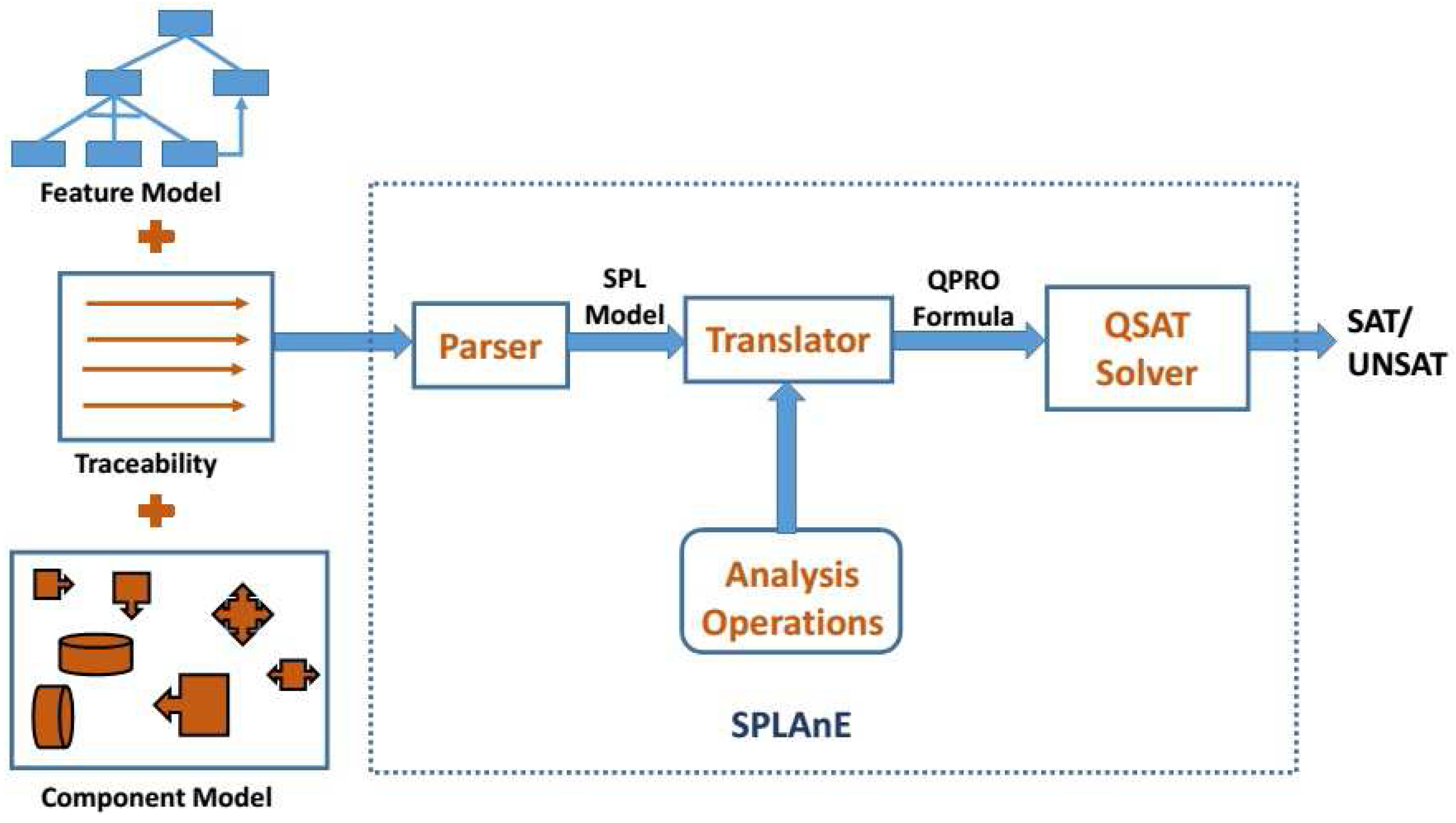
• We present a tool named SPLAnE that enables SPL developers to perform existing operations in the literature over feature diagrams [6] and many new operations proposed in this paper. It also allows one to perform analysis operations on a component model and SPL model. We used the FaMa framework to develop SPLAnE that makes it flexible to extend with new analyses of specific needs.
• We experimented on our approach with a number of models, i.e.,: (i) real and large Debian models; (ii) randomly-generated SPL models from ten features to twenty thousand features with different levels of cross-tree constraints; and (iii) SPLOTrepository models. The experimental results also give the comparison across two QSAT solvers (CirQit and RaReQS) and three SAT solvers (Sat4j, PicoSAT and MiniSAT).
• An example from the cloud computing domain is presented to motivate the practical usefulness of the proposed approach.

The remainder of the paper is organized as follows: Section 2 shows a motivating scenario for using SPLAnE ; Section 3 presents the tool SPLAnE , which is implemented based on the proposed approach; Section 4 describes different analysis operations to extract information by using the SPLAnE tool; Section 5 analyzes empirical results from experiments that evaluate the scalability of SPLAnE ; Section 6 compares our approach to related work; and finally, Section 8 presents concluding remarks.

2. Motivating Example

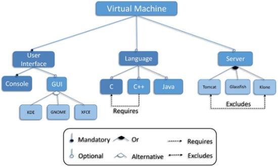
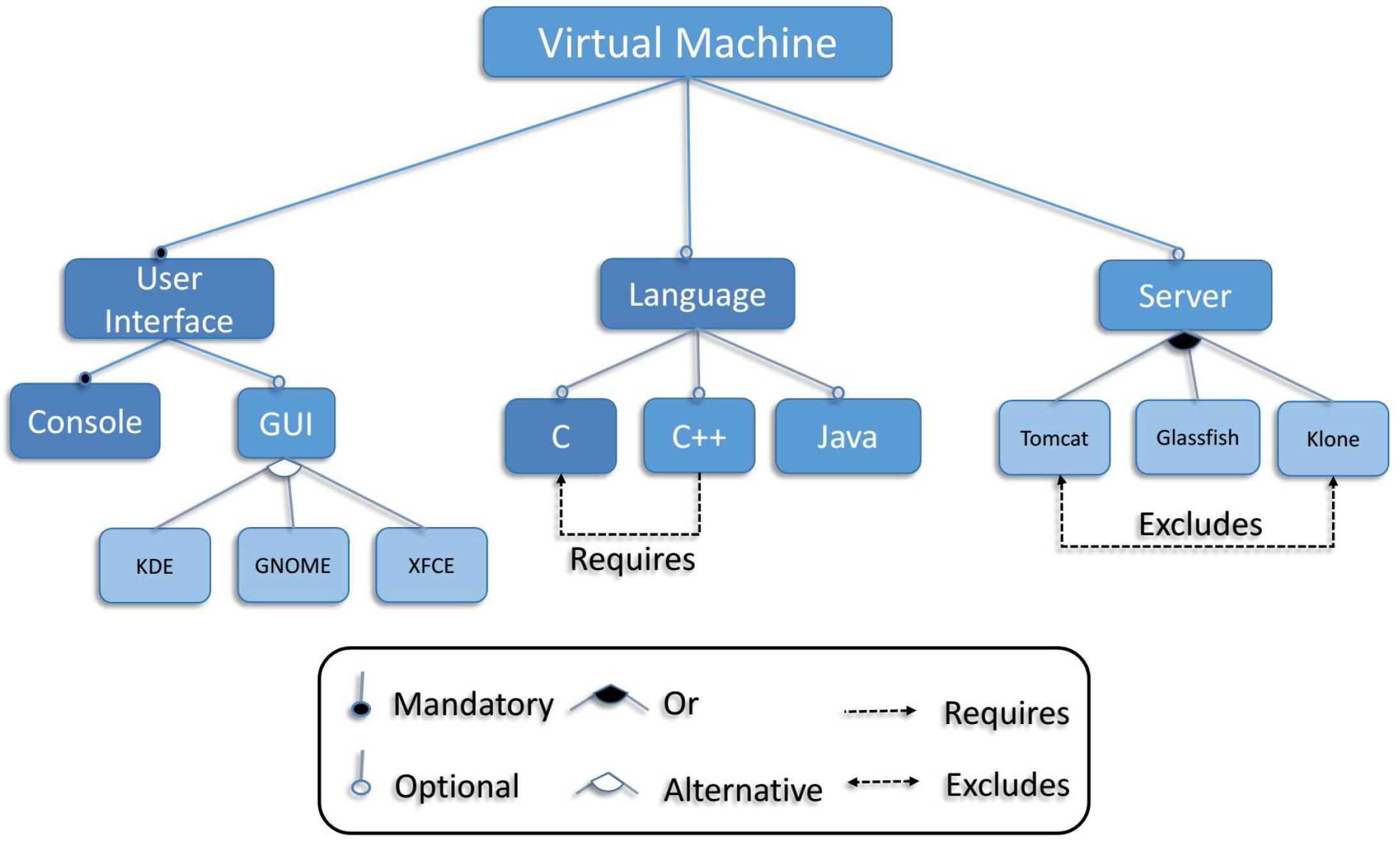
In this paper, we present cloud computing as a product line. The feature model and the component model are used to manage the variability across the scope and core assets, respectively.

Feature Models

Feature models have been used to describe the variant and common parts of the product line since Kang [29] has defined them. The sets of possible valid combinations of those features are represented by using different constraints among features. The feature model in Figure 1 represents the features provided by the cloud computing. Two different kinds of relationships are used: (i) hierarchical relationships, which describe the options for variation points within the product line; and (ii) cross-tree constraints that represent constraints among any features of the feature tree. Different notations have been proposed in the literature [6]; however, most of them share the following relationship flavors:

Four different hierarchical relationships are defined:

• mandatory: this relationship refers to features that have to be in the product if its parent feature is in the product. Note that a root feature is always mandatory in feature models.
• optional: this relationship states that a child feature is an option if its parent feature is included in the product.
• alternative: it relates a parent feature and a set of child features. Concretely, it means that exactly one child feature has to be in the product if the parent feature is included.
• or: this relationship refers to the selection of at least one feature among a group of child features, having a similar meaning to the logical OR.

Later, two kinds of cross-tree relationships are used:

• requires: this relationship implies that if the origin feature is in the product, then the destination feature should be included.
• excludes: this relationship between two features implies that, only one of the feature can be present in a product.

Cloud computing technology provides ready to use infrastructure for the clients. The cloud system reduces the cost of maintaining the hardware and software, and also reduces the time to build the infrastructure on the client side. The client pays only for the hardware and software used based on the duration. The feature model for cloud computing is shown in Figure 1. The root feature $VirtualMachine$ is a mandatory feature by default. The mandatory relationship is present between the feature $VirtualMachine$ and $UserInterface$, so the feature $UserInterface$ has to be present if feature $VirtualMachine$ is present in the product. The optional relationship is present between the feature $Language$ and $VirtualMachine$, so it is optional to have feature $Language$ in the products. The feature $GUI$ has alternative relationship with its child features $\{KDE,GNOME,XFCE\}$. Hence, if feature $GUI$ is selected in a product, then only one of its child feature has to be present in that product. The feature $Server$ has or relationship with its child features $\{Tomcat,Glassfish,Klone\}$. Hence, if feature $Server$ is selected in a product, then at least one of its child feature has to be present in that product. The feature $C$++ requires the feature C to be present in a product. The presence of feature $Tomcat$ in a product does not allow the feature $Klone$ and vice versa. The client can request for a system with the set of features called a $specification$. The minimum set of features in the specification should contain features $\{VirtualMachine$, $UserInterface$, $Console\}$ as they are mandatory features. We can term this as commonality across all the products of an SPL. The specification F = {$VirtualMachine$, $UserInterface$, $Console$, $GUI$, $KDE$, $Language$, $C\}$ is valid for the creation of a virtual machine because it satisfies all the constraints in the feature model. The specification F = {$VirtualMachine$, $UserInterface$, $Console$, $GUI$, $KDE$, $Language$, $C$++} is not valid because it contains a feature $C$++ so it is necessary to select feature C.

Component model: Similar to a feature model, same notations can be used to represent variability amongst the components present in $core$ $assets$ of an SPL, we call it a Component Model (CM). The variability amongst the components can also be represented by any other models like the Orthogonal Variability Model (OVM), Varied Feature Diagram (VFD) and Free Feature Diagrams (FFDs) [20,30]. The component model in Figure 2 represents the resources available to create a virtual machine. The cloud computing technology will create a virtual machine that contains a set of components required to implement the features present in the client $specification$. Such set of components is called an $implementation$. The implementation C = $\{LinuxCore,$ $IUser,$ $IConsole,$ $Terminal,$ $ILanguage,$ $\mathit{\text{C-lang}},$ $\mathit{\text{c-lib}}$} is valid because it satisfies all the constraints on the component model, so a virtual machine can be created with these components. The implementation C = $\{LinuxCore,$ $IUser,$ $IConsole,$ $ILanguage,$ $\mathit{\text{C-lang}},$ $\mathit{\text{c-lib}}$} is invalid, because the component $Terminal$ or $XTerminal$ or both are required to satisfy the component model constraints.

Table 1. Traceability relation for the virtual machine.

Feature	Components	Feature	Components
$VirtualMachine$	$\left\{\right\{LinuxCore\left\}\right\}$	$f_1$	$\left\{\left\{c_1\right\}\right\}$
$UserInterface$	$\left\{\right\{IUser\left\}\right\}$	$f_2$	$\left\{\left\{c_2\right\}\right\}$
$Language$	$\left\{ILanguage\right\}$	$f_8$	$\left\{\left\{c_{14}\right\}\right\}$
$Server$	$\left\{\right\{IServer\left\}\right\}$	$f_{12}$	$\left\{\left\{c_{10}\right\}\right\}$
$Console$	$\left\{\right\{IConsole,XTerminal\},$	$f_3$	$\{\{c_3,c_4\},\{c_3,c_5\}\}$
	$\{IConsole,Terminal\}\}$
$GUI$	$\left\{\right\{IGUI\left\}\right\}$	$f_4$	$\left\{\left\{c_6\right\}\right\}$
$KDE$	$\left\{\right\{KDEApp\left\}\right\}$	$f_5$	$\left\{\left\{c_7\right\}\right\}$
$GNOME$	$\left\{\right\{GNOMEApp\left\}\right\}$	$f_6$	$\left\{\left\{c_8\right\}\right\}$
$XFCE$	$\left\{\right\{XFCEApp\left\}\right\}$	$f_7$	$\left\{\left\{c_9\right\}\right\}$
C	$\left\{\right\{\mathit{\text{C-lang}},\mathit{\text{c-lib}}\left\}\right\}$	$f_9$	$\left\{\{c_{15},c_{16},c_{17}\}\right\}$
$C$++	$\left\{\right\{\mathit{\text{C-lang}},\mathit{\text{c-lib}},gcc,c++lib\left\}\right\}$	$f_{10}$	$\left\{\{c_{15},c_{16},c_{17},c_{20}\}\right\}$
$Java$	$\left\{\right\{OpenJDK\},\{OracleJDK\left\}\right\}$	$f_{11}$	$\{\left\{c_{18}\right\},\left\{c_{19}\right\}\}$
$Tomcat$	$\left\{\right\{TomcatApp\left\}\right\}$	$f_{13}$	$\left\{\left\{c_{11}\right\}\right\}$
$Glassfish$	$\left\{\right\{GlassfishApp\left\}\right\}$	$f_{14}$	$\left\{\left\{c_{12}\right\}\right\}$
$Klone$	$\left\{\right\{KloneApp\left\}\right\}$	$f_{15}$	$\left\{\left\{c_{13}\right\}\right\}$

shows the traceability relation between the features and the components. The entry in the row of feature $Glassfish$ means the component $GlassfishApp$ implements the feature $Glassfish$. Similarly, the feature $Console$ can be implemented by the set of components: $\{IConsole,XTerminal\}$ or $\{IConsole,Terminal\}$. For each feature in the client specification, the traceability relation gives the required sets of components. In the feature model, the effective features are only the leaf features. The traceability of a parent feature like the feature $GUI$ can be implemented by the set of components: $\left\{IGUI\right\}$. The feature $GUI$ can be abstracted by eliminating all of its child features $\{KDE,GNOME,XFCE\}$; this allows to analyze the SPL at a higher level of abstraction. Section 3 refers to Columns 3 and 4 from Table 1 to represent the short name for features and components respectively.

Figure 3 shows the four preconfigured virtual machines. The preconfigured machines show the set of components from the component model shown in Figure 2.

Software product lines can contain a large set of different products. Therefore, facing the complexity of the feature models that represent the products within an SPL is hard. To help in such a difficult task, researchers rely on the computer-aided extraction of information from feature models. This extraction is usually known as the automated analysis in the area. To reason about those models, the relationships existing in the feature model are processed through a CSP (Constraint Satisfaction Problem), SAT, BDD (Binary Decision Diagrams) solver or a specific algorithm. Later, the operation is used to extract specific information from the model. An SPL with twelve leaf features can result in a search space of $2^{12}$ possible products. Analysis of such a huge search space is a non-trivial task. Some interesting analyses that could performed in this scenario of a Virtual Machine Product Line (VMPL) are as follows:

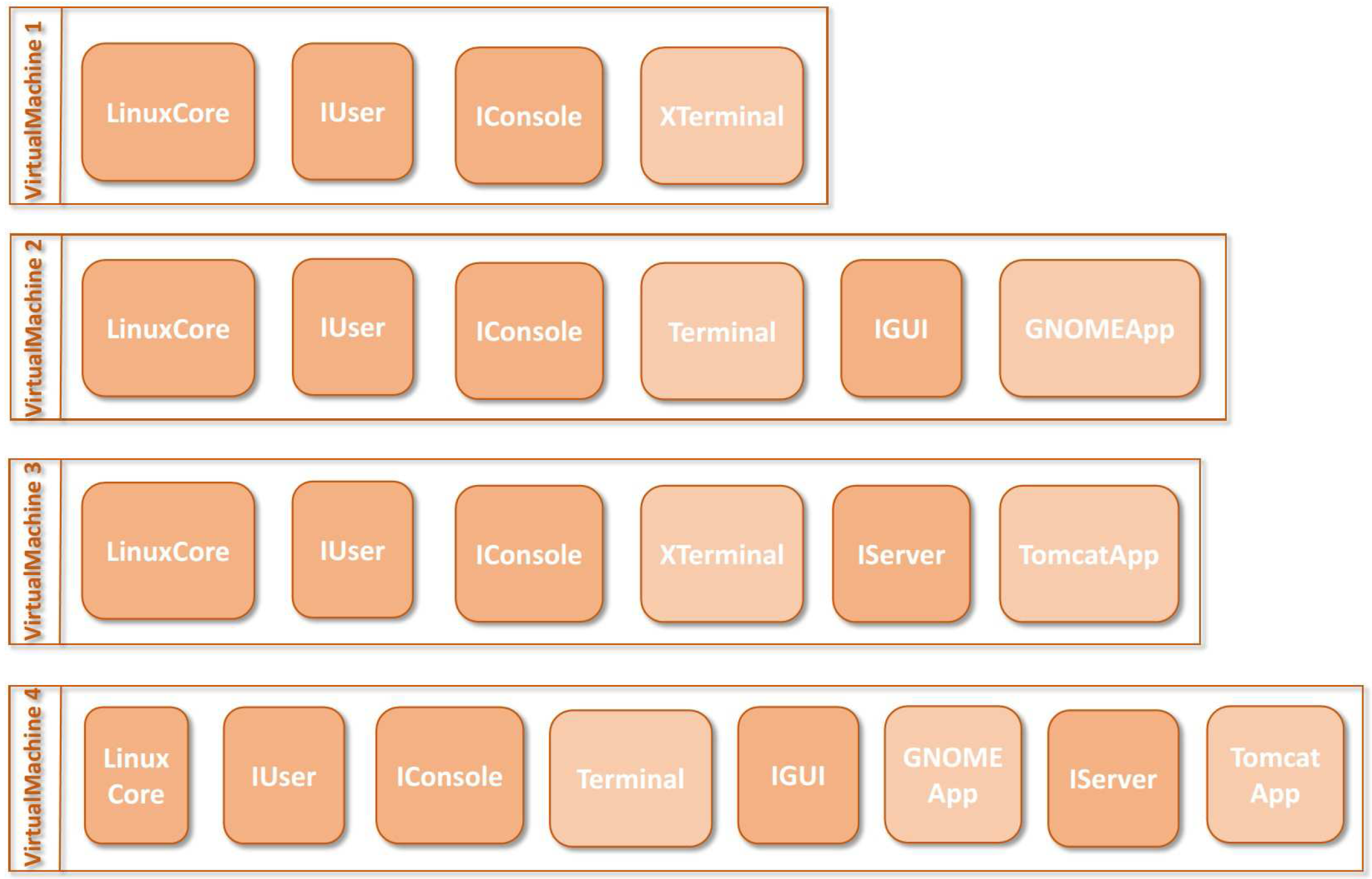
• Check if at least one of the pre-configured machines covers the needs of a new user configuration: In VMPL, there is always a need to check the existence of any virtual machine as per the given user specification. For example, the specification F=$\{VirtualMachine,$ $UserInterface,$ $Console,$ $GUI,$ $GNOME\}$ should be first analyzed to check the existence of any implementation that implements F. The implementation C=$\{LinuxCore,$ $IUser,$ $IConsole,$ $Terminal,$ $IGUI,$ $GNOMEApp,$ $IServer,$ $TomcatApp\}$ (equivalent to preconfigured Virtual Machine 2 in Figure 3) provides all the features in the specification F, it means that there exists a pre-configured machine which covers the user specification F.
• Check if at least one of the pre-configured machines realizes (exactly) the needs of a new user configuration: Multiple implementations may cover a given user specification F. We can analyze the VMPL to find the realized implementation for the user specification. For example, the implementation C=$\{LinuxCore,$ $IUser,$ $IConsole,$ $Terminal,$ $IGUI,$ $GNOMEApp\}$ (equivalent to preconfigured Virtual Machine 3 in Figure 3) exactly provides all the feature in the specification F.
• Check if there are dead packages: Actual VMPLs contain a huge number of components for Linux systems. The components that are not present in any of the products are termed as dead elements in the product line. In the given VMPL, none of the components is dead.

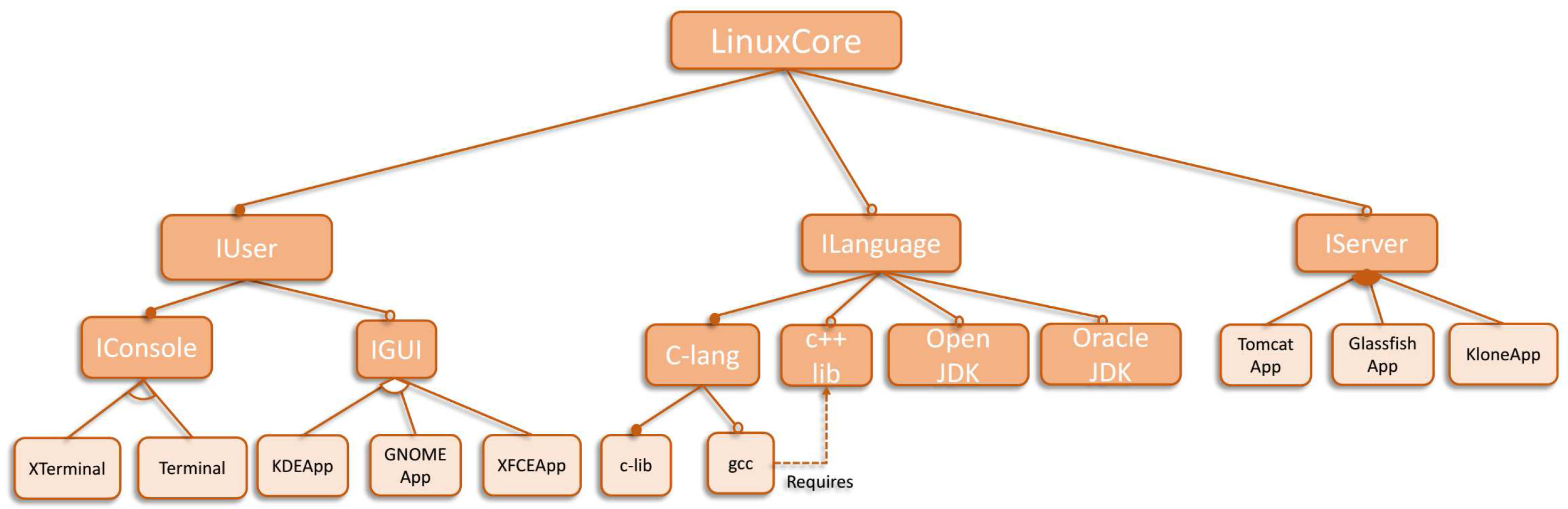
3. SPLAnE Framework: Traceability and Implementation

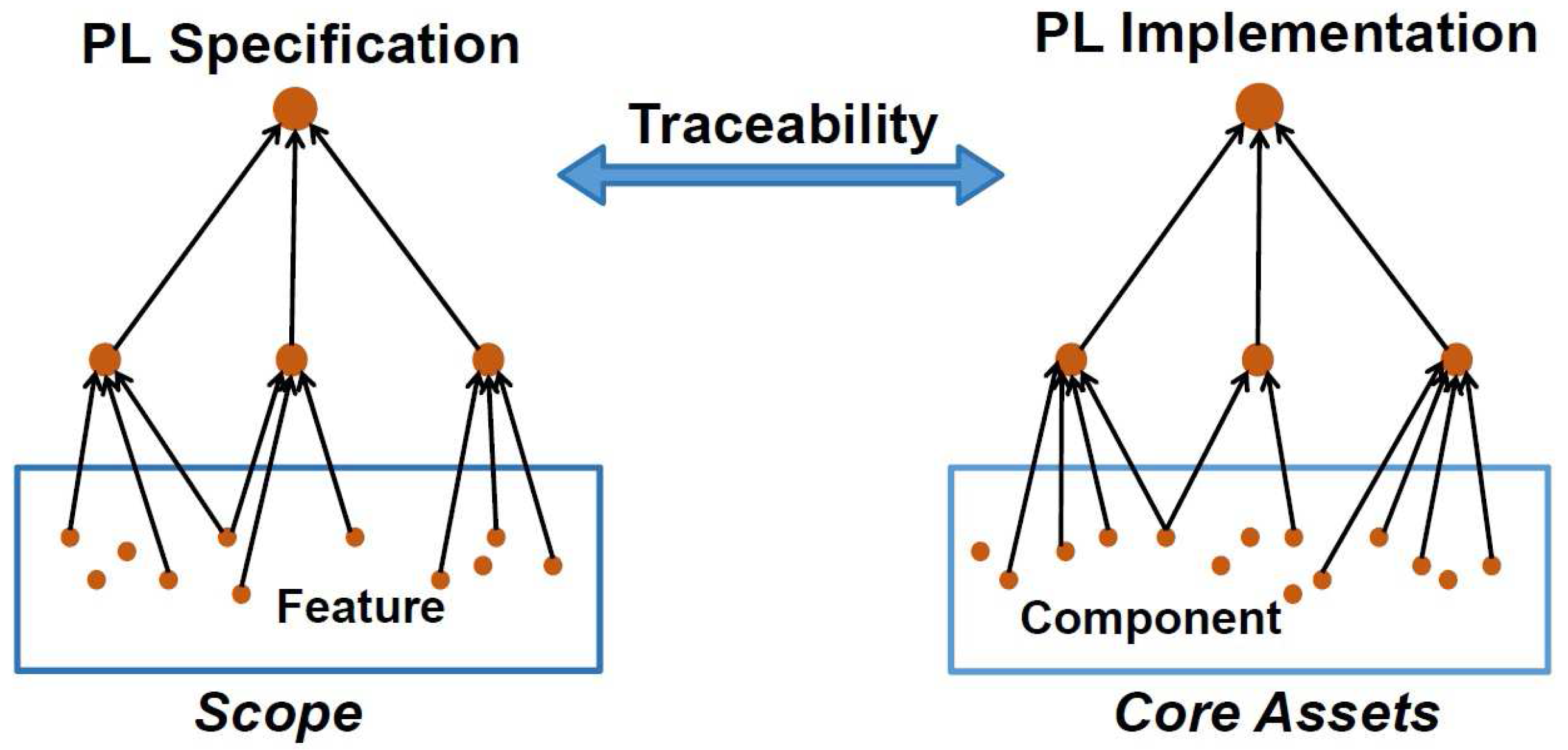
3.1. Specification and Implementation

The set of all features found in any of the products in a product line defines the scope of the product line. We denote the scope of a product line by $\mathcal{F}$. A scope $\mathcal{F}$ consists of a set of features, denoted by small letters $f_1,f_2\cdots$. Specifications are subsets of features in the scope and are denoted by $F_1,F_2,\cdots$, with possible subscripts. On the other hand, the collection of components in the product line defines the core assets and is denoted as $\mathcal{C}$. Small letters $c_1,c_2\cdots$, etc. represent components. Implementations (subsets of components) are denoted by capital letters $C_1,C_2\cdots$ with possible subscripts. A Product Line (PL) specification is a set of $specifications$ in an SPL, denoted as $\overline{\mathcal{F}}$∈$\wp ($$\wp ($$\mathcal{F}$$)\backslash$$\left\{\varnothing \right\})$. Similarly, a Product Line (PL) implementation is denoted as $\overline{\mathcal{C}}\in \wp (\wp \left(\mathcal{C}\right)\backslash \left\{\varnothing \right\})$. In VMPL, the scope, core assets, specifications and implementations are as follows:

• Scope $\mathcal{F}=$$\{f_1:VirtualMachine,$ $f_2:UserInterface,$ $f_3:Console,$ $f_4:GUI,$ $f_5:KDE,$ $f_6:GNOME,$ $f_7:XFCE,$ $f_8:Language,$ $f_9:C,$ $f_{10}:C$++, $f_{11}:Java,$ $f_{12}:Server,$ $f_{13}:Tomcat,$ $f_{14}:Glassfish,$ $f_{15}:Klone$}
• Core Assets $\mathcal{C}=$$\{c_1:LinuxCore,$ $c_2:IUser,$ $c_3:IConsole,$ $c_4:XTerminal,$ $c_5:Terminal,$ $c_6:IGUI,$ $c_7:KDEApp,$ $c_8:GNOMEApp,$ $c_9:XFCEApp,$ $c_{10}:IServer,$ $c_{11}:TomcatApp,$ $c_{12}:GlassfishApp,$ $c_{13}:KloneApp,$ $c_{14}:ILanguage,$ $c_{15}:\mathit{\text{C-lang}},$ $c_{16}:\mathit{\text{c-lib}},$ $c_{17}:gcc,$ $c_{18}:OpenJDK,$ $c_{19}:OracleJDK,$ $c_{20}:c++lib$}
• PL Specification $\overline{\mathcal{F}}$={
  $F_1:$$\{VirtualMachine,$ $UserInterface,$ $Console$} or $\{f_1,$ $f_2,$ $f_3\}$,
  $F_2:$$\{VirtualMachine,$ $UserInterface,$ $Console,$ $GUI,$ $KDE$} or $\{f_1,$ $f_2,$ $f_3,$ $f_4,$ $f_5$},
  $F_3:$$\{VirtualMachine,$ $UserInterface,$ $Console,$ $Server,$ $Tomcat,$ $Glassfish$} or $\{f_1,$ $f_2,$ $f_3,$ $f_{12},$ $f_{13},$ $f_{14}$ },
  $F_4:$$\{VirtualMachine,$ $UserInterface,$ $Console,$ $GUI,$ $KDE,$ $Server,$ $Tomcat$} or $\{f_1,$ $f_2,$ $f_3,$ $f_4,$ $f_5,$ $f_{12},$ $f_{13}$},
  $F_5:$$\{VirtualMachine,$ $UserInterface,$ $Console,$ $GUI,$ $KDE,$ $Language,$ $Java,$ $Server,$ $Tomcat$} or $\{f_1,$ $f_2,$ $f_3,$ $f_4,$ $f_5,$ $f_8,$ $f_{11},$ $f_{12},$ $f_{13}$}
  }, where $F_1,F_2,F_3$, $F_4$ and $F_5$ are some specifications.
• PL Implementation $\overline{\mathcal{C}}$={
  $C_1:$$\{LinuxCore,$ $IUser,$ $IConsole,$ $XTerminal$} or $\{c_1,$ $c_2,$ $c_3,$ $c_4$$\},$
  $C_2:$$\{LinuxCore,$ $IUser,$ $IConsole,$ $Terminal$} or $\{c_1,$ $c_2,$ $c_3,$ $c_5$$\},$
  $C_3:$$\{LinuxCore,$ $IUser,$ $IConsole,$ $Terminal,$ $IGUI,$ $KDEApp$} or $\{c_1,$ $c_2,$ $c_3,$ $c_5,$ $c_6,$ $c_7$$\},$
  $C_4:$$\{LinuxCore,$ $IUser,$ $IConsole,$ $Terminal,$ $IServer,$ $TomcatApp,$ $GlassfishApp$} or $\{c_1,$ $c_2,$ $c_3,$ $c_5,$ $c_{10},$ $c_{11},$ $c_{12}$$\},$
  $C_5:$$\{LinuxCore,$ $IUser,$ $IConsole,$ $Terminal,$ $IGUI,$ $KDEApp,$ $IServer,$ $KloneApp,$ $Glassfish$} or $\{c_1,$ $c_2,$ $c_3,$ $c_5,$ $c_6,$ $c_7,$ $c_{10},$ $c_{12},$ $c_{13}$$\},$
  $C_6:$$\{LinuxCore,$ $IUser,$ $IConsole,$ $Terminal,$ $IGUI,$ $KDEApp,$ $IServer,$ $TomcatApp,$ $Glassfish$} or $\{c_1,$ $c_2,$ $c_3,$ $c_5,$ $c_6,$ $c_7,$ $c_{10},$ $c_{11},$ $c_{12}$$\},$
  $C_7:$$\{LinuxCore,$ $IUser,$ $IConsole,$ $Terminal,$ $IGUI,$ $KDEApp,$ $ILang,$ $OpenJDK,$ $IServer,$ $TomcatApp$} or $\{c_1,$ $c_2,$ $c_3,$ $c_5,$ $c_6,$ $c_7,$ $c_{14},$ $c_{18},$ $c_{10},$ $c_{11}$}
  }, where $C_1$ to $C_7$ are some implementations.

3.2. Traceability

We present a formalism for two variation of traceability relation: (i) $1:M$ mapping and (ii) $N:M$ mapping. In traceability relation, $1:M$ mapping is between a feature and a set of component sets, were as $N:M$ is a mapping between feature set and a set of component sets.

Traceability with $1:M$ mapping: A feature is implemented using a set of non-empty subset of components in the core asset $\mathcal{C}$. This relationship is modeled by the partial function $\mathcal{T}:\mathcal{F}\to \wp \left(\wp \right(\mathcal{C})\backslash \{\varnothing \left\}\right)$. When $\mathcal{T}\left(f\right)=\{C_1,C_2,C_3\}$, we interpret it as the fact that the set of components $C_1$ (also, $C_2$ and $C_3$) can implement the feature f. When $\mathcal{T}\left(f\right)$ is not defined, it denotes that the feature f does not have any components to implement it.

Traceability with $N:M$ mapping: A set of features can be implemented using a set of non-empty subset of components in the core asset $\mathcal{C}$. This relationship is modeled by the partial function $\mathcal{T}:\left(\wp \right(\mathcal{F})\backslash \{\varnothing \left\}\right)\to \wp \left(\wp \right(\mathcal{C})\backslash \{\varnothing \left\}\right)$. It may happen that, two features $f_1$ and $f_2$ can be implemented by a single component $c_1$. In this case, $\mathcal{T}\left(\{f_1,f_2\}\right)=\left\{C_1\right\}$, where $C_1=\left\{c_1\right\}$.

Definition 1 (SPL). 

An SPL Ψ is defined as a triple $\langle \overline{\mathcal{F}},\overline{\mathcal{C}},\mathcal{T}\rangle$, where $\overline{\mathcal{F}}\in \wp (\wp \left(\mathcal{F}\right)\backslash \left\{\varnothing \right\})$ is the PL specification, $\overline{\mathcal{C}}\in \wp (\wp \left(\mathcal{C}\right)\backslash \left\{\varnothing \right\})$ is the PL implementation and $\mathcal{T}$ is the traceability relation.

3.3. The Implements Relation

A feature is implemented by a set of components C, denoted $implements(C,f)$, if C includes a non-empty subset of components $C^{\prime }$ such that $C^{\prime }\in \mathcal{T}\left(f\right)$. It is obvious from the definition that if $\mathcal{T}\left(f\right)=\varnothing$, then f is not implemented by any set of components. In VMPL, $f_5$ is implemented by implementations $C_3$, $C_5$, $C_6$ and $C_7$, but not by implementations $C_1$, $C_2$ and $C_4$.

In order to extend the definition to specifications and implementations, we define a function $Provided\_by\left(C\right)$ which computes all the features that are implemented by C: $Provided\_by\left(C\right)$ = $\{f\in \mathcal{F}|implements(C,f)\}$. In VMPL, $Provided\_by\left(C_1\right)=\{f_1,f_2,f_3\}$ and $Provided\_by\left(C_3\right)=\{f_1,f_2,f_3,f_4,f_5\}$. With the basic definitions above, we can now define when an implementation exactly implements a specification.

Definition 2 (Realizes). 

Given $C\in \overline{\mathcal{C}}$ and $F\in \overline{\mathcal{F}}$, $Realizes(C,F)$ if $F=Provided\_by\left(C\right)$.

The $realizes$ definition given above is rather strict. Thus, in the above example, the implementation $C_3$ realizes the specification $F_2$, but it does not realize $F_1$ even though it provides an implementation of all the features in $F_1$. In many real-life use-cases, due to the constraints on packaging of components, the exactness may be restrictive. We relax the definition of Realizes in the following.

Definition 3 (Covers). 

Given $C\in \overline{\mathcal{C}}$ and $F\in \overline{\mathcal{F}}$, $Covers(C,F)$ if $F\subseteq Provided\_by\left(C\right)$ and $Provided\_by\left(C\right)\in \overline{\mathcal{F}}$.

The additional condition ($Provided\_by\left(C\right)\in \mathcal{F}$) is added to address a tricky issue introduced by the Covers definition. Suppose the scope $\mathcal{F}$ consisted of only two specifications $\left\{f_1\right\}$ and $\left\{f_2\right\}$. Let’s say that the two variants ($f_1$ and $f_2$) are mutually exclusive features. The implementation $C=\{c_1,c_2\}$ implements the feature $f_1$, assuming $\mathcal{T}\left(f_1\right)=\left\{\left\{c_1\right\}\right\}$ and $\mathcal{T}\left(f_2\right)=\left\{\left\{c_2\right\}\right\}$. Without the provision, we would have $Covers(C,\left\{f_1\right\})$. However, since $Provided\_by\left(C\right)=\{f_1,f_2\}$, it actually implements both the features together, thus violating the requirement of mutual exclusion. In the VMPL, the implementation $C_6$ covers the specifications $F_1$, $F_2$, $F_3$ and $F_4$. The set of products of the SPL is now defined as the specifications and the implementations covering them through the traceability relation.

Definition 4 (SPL Products). 

Given an SPL $\mathrm{\Psi }=\langle \overline{\mathcal{F}},\overline{\mathcal{C}},\mathcal{T}\rangle$, the products of the SPL, denoted by a function $Prod\left(\mathrm{\Psi }\right)$ which generate a set of all specification-implementation pairs $\langle F,C\rangle$ where $Covers(C,F)$.

Thus, in the VMPL example, we see that there are many potential products. Valid products are $\langle C_1,F_1\rangle ,\langle C_2,F_1\rangle$, $\langle C_3,F_1\rangle$, $\langle C_3,F_2\rangle$, $\langle C_4,F_1\rangle$, $\langle C_4,F_3\rangle$⋯.

4. Analysis Operations

Given an SPL $\mathrm{\Psi }=\langle \overline{\mathcal{F}},\overline{\mathcal{C}},\mathcal{T}\rangle$, we define the following analysis problems. The problems center around the new definition of an SPL product.

4.1. SPL Model Verification

Questions: Is it a valid SPL model? Is it a void SPL model? Is the SPL model complete? 

A given SPL model $\mathrm{\Psi }=\langle \overline{\mathcal{F}},\overline{\mathcal{C}},\mathcal{T}\rangle$ is valid, if there exists a specification and implementation. Let’s assume a feature model with three features $f_1$, $f_2$ and $f_3$. The feature $f_1$ is the root and the features $f_2$ and $f_3$ are the mandatory children of $f_1$. An $excludes$ relation exists between $f_2$ and $f_3$. The feature model cannot have any specification because of $excludes$ relation and such SPL model is not a $validmodel$. An SPL models should be validated before analyzing any operations over it. Large and complex SPLs undergoes continuous modification, such SPLs has to be verified for its validity after every modification. In case of VMPLs, after adding new features, components and cross-tree constraints, a validity of model should be tested. “Is the virtual machine feature model and component model valid?”, such questions must be verified before further analysis of VMPL.

If all the features have a traceability relation with the components which implement them, such a traceability relation is called as $completetraceabilityrelation$. If there exists a feature which does not have a traceability relation with any components, then such a traceability relation is called an $incompletetraceabilityrelation$. When a SPLs are under development, all the features many not have its corresponding components developed. The operation $completetraceabilityrelation$ help us to identify such features and proceed for its components development. The preliminary properties $validmodel$ and $completetraceabilityrelation$ should hold before analyzing any other properties. Let us assume an SPL model $\langle \overline{\mathcal{F}},\overline{\mathcal{C}},\mathcal{T}\rangle$ which is a $validmodel$ but none of the implementations $C_i$ cover any of the specification $F_j$. Such a model is called $voidproductmodel$, i.e., the model is not able to return a single product. In SPL model, it may happen that a feature model is valid, a component model is valid and a traceability is also complete, but the SPL model is not able to generate a single product. This is possible if no specification covers any of the implementation. A question like, “Do a Virtual Machine Product Line can generate at least one virtual machine ?” is very important to conduct further analysis of a product line.

4.2. Complete and Sound SPL

Question: Does the SPL model is adequate for all the user specifications? Do all implementation has it corresponding specification? Which are the useful implementations? Is there at least one implementation which realizes a given user specification? 

The completeness property of the SPL relates to the implementability of a specification. A specification F is implementable if there is an implementation C such that $Covers(C,F)$. Completeness determines if the PL implementation (set of implementation variants) is adequate to provide implementations for all the variant specifications in the PL specification. An SPL $\langle \overline{\mathcal{F}},\overline{\mathcal{C}},\mathcal{T}\rangle$ is complete if for every $F\in \overline{\mathcal{F}}$, there is an implementation $C\in \overline{\mathcal{C}}$ such that $Covers(C,F)$. The soundness property relates to the usefulness of an implementation in an SPL. An implementation is said to be useful if it implements some specification in the scope. An SPL $\langle \overline{\mathcal{F}},\overline{\mathcal{C}},\mathcal{T}\rangle$ is sound if for every $C\in \overline{\mathcal{C}}$, there is a specification $F\in \overline{\mathcal{F}}$ such that $Covers(C,F)$. The complete and sound are very crucial properties of any SPLs. Does a VMPL is able to provide a virtual machine for every valid requirements (specifications) from users?, if YES then the VMPL is complete. If there is some specification which cannot be implemented by any of the implementation in the PL implementation, then such PL implementation is not adequate to fill the wish of all the user specifications. In VMPL, there may be such requirements for which no virtual machine can be generated. In such case, either feature model, component model or traceability relation should be analyzed to figure out the actual problem. On the other hand, PL implementation may provide huge set of implementation where as PL specification may be answered by a subset of PL implementation. In case of VMPL, we may end up with such virtual machine which may not get covered by any of the user specifications. Such machine should be removed from the pre-configured machine list.

4.3. Product Optimization

Questions: Do the given specification and implementation, forms a product? Is there an implementation which provide all the features in a given user specification? Is there an implementation exactly meeting a given user specification? Is there only one implementation for a given specification? 

Given a specification, we want to find out all the variant implementations that cover the specification. This is given by a function $FindCovers\left(F\right)$$=$$\left\{C\right|$$Covers(C,F)\}$. At times, it is necessary for a premier set of features to be provided exactly for some product variants. For example, a client company with a critical usage of the product would limit the risk of feature interaction. In this case, we want to find out if there is an implementation that realizes the specification. A specification is existentially explicit if there exists an implementation C such that $Realizes(C,F)$. Dually, it is universally explicit if for all implementations $C\in \overline{\mathcal{C}}$, $Covers(C,F)$ implies $Realizes(C,F)$. Multiple implementations may implement a given specification. This may be a desirable criterion of the PL implementation from the perspective of optimization among various choices. Thus, the specifications which are implemented by only a single implementation are to be identified. $F\in \overline{\mathcal{F}}$ has a unique implementation if $\left|FindCovers\right(F\left)\right|=1$.

Is there a virtual machine which provide all the features as per the client specification? A covers is more relaxed version where a specification is implemented by an implementation, but the implementation may contain extra components which may not require to implement any of the features in a specification. It may happen that, the cloud may have such pre-configured virtual machines which provides all the features as per user specifications. Furthermore, this pre-configured machines has extra components which are not required to support any of the features in user specifications. This may results in redundancy of components in a virtual machine. Is there a virtual machine which provide exactly all the features as per the client specification? The tighter version of cover is realize, which strictly does not allow any extra components which are not required for features implementation present in a specification. A realize is the optimized version of cover operation. Finding the optimized virtual machine on cloud which match the exact user specifications is achieved by realize. Is there at least one virtual machine which provides exactly all the features as per the client specification? The existentially explicit operations guarantee the presence of at least one implementation which is realized by a given specifications. It means, in VMPL for a user specification there exists at least one virtual machine which realizes it and this guarantees the presence of at least one optimized configuration. The universally explicit is the tighter version of existentially explicit, which means all the implementation covers by a given specification implies that it is an realization. For universally explicit specifications, cloud always produce the optimized virtual machine. Does a given user specification has only one virtual machine provided by cloud? In VMPL, there may be some specification which is covered by only one virtual machine, such implementations are unique.

4.4. SPL Optimization

Questions: Does an element is present across all the products? Does an element is used in at least single product? Does an element not in use? Which all elements are redundant in a given product? Which are the extra features provided by a product apart from the given user specification? 

Identification of common, live and dead elements in an SPL are some of the basic analyses operations in the SPL community. We redefine these concepts in terms of our notion of products: An element e is common if for all $\langle F,C\rangle \in Prod\left(\mathrm{\Psi }\right)$, $e\in F\cup C$. An element e is live if there exists $\langle F,C\rangle \in Prod\left(\mathrm{\Psi }\right)$ such that $e\in F\cup C$. An element e is dead if for all $\langle F,C\rangle \in Prod\left(\mathrm{\Psi }\right)$, $e\notin F\cup C$. Now a days with the advance in technology, business changes it requirements so quickly that, exiting products in market get replaced by another advance products in a very short time span. As the SPLs evolves, new cross-tree constraints get added or removed, this results in change of products. Due to such modification, few features or components in SPL may become live or dead. Do the component c is present in at least one virtual machine provided by VMPL? Do the component c is not present in any of the virtual machines provided by VMPL? The common property find all the common elements (features or components) across all the products. This operation is required to create a common platform for a SPL. Do the component c is present in all the virtual machines provided by VMPL?

There may be certain implementations that are useful but the implementable specifications are not affected if these implementations are dropped from the PL implementation. These implementations are called superfluous. Formally, an implementation $C\in \overline{\mathcal{C}}$ is superfluous if for all $F\in \overline{\mathcal{F}}$ such that $Covers(C,F)$, there is a different implementation $D\in \overline{\mathcal{C}}$ such that $Covers(D,F)$. Superfluousness is relative to a given PL implementation. If in an SPL Ψ, $\overline{\mathcal{F}}=\left\{\left\{f\right\}\right\}$, $\overline{\mathcal{C}}=\{\left\{a\right\},\left\{b\right\}\}$ and $\mathcal{T}\left(f\right)=\left\{\right\{a\},\{b\left\}\right\}$, then both the implementations $\left\{a\right\}$ and $\left\{b\right\}$ are superfluous with respect to Ψ, whereas if either $\left\{a\right\}$ or $\left\{b\right\}$ is removed from the PL implementation, the remaining implementation ($\left\{b\right\}$ or $\left\{a\right\}$) is not superfluous anymore (with respect to the reduced SPL). The feature Java in VMPL, can be implemented by component OpenJDK or OracleJDK. Such traceability results in many superfluous implementations . Superfluousness for a specification guarantees the presence of alternate implementations.

Which are the components in the virtual machines that can be removed without impacting the user specification? A component is redundant if it does not contribute to any feature in any implementation in the SPL. A component $c\in \mathcal{C}$ is redundant if for every $C\in \overline{\mathcal{C}}$, we have $Provided\_by\left(C\right)=Provided\_by(C\backslash \{c\left\}\right)$. An SPL can be optimized by removing the redundant components without affecting the set of products. Redundant elements may not be dead. Due to the packaging, redundant elements can be part of useful implementations of the SPL and hence be live. Do the component c is required for any of the features in a user specification? A component c is critical for a feature f in the SPL scope $\mathcal{F}$, when the component must be present in an implementation that implements the feature f: for all implementations $C\in \overline{\mathcal{C}}$, $(c\notin C\Rightarrow \neg implements(C,f\left)\right)$. This definition can be extended to specifications as well: a component c is critical for a specification F, if for all implementations $C\in \overline{\mathcal{C}}$, $(c\notin C\Rightarrow \neg Covers(C,F\left)\right)$. A virtual machine may contain components which may not be required for any of the features in a user specifications, but it may remain due to packaging. Such components are redundant but not critical.

Can virtual machine provide more features with the same set of components? When a specification is covered (but not realized) by an implementation, there may be extra features (other than those in the specification) provided by the implementation. These extra features are called extraneous features of the implementation. Since there can be multiple covering implementations for the same specification, we get different choices of implementation and extraneous features pairs: $Extra\left(F\right)\equiv \left\{\langle C,Provided\_by\left(C\right)\backslash F\rangle \right|Covers(C,F)\}$. User may demand for virtual machines with some specification. The available pre-configured machine provide all the features in user specification, and also provide few more features which are extraneous.

4.5. Generalization and Specialization in SPL

Questions: Do the union of two or more products result in a new product? What is the difference between two products? 

In an SPL, sometimes there is a need to check the $aggregation$ relationship between the specifications, implementations or products. Is there a virtual machine which has features provided by a given set of virtual machines? The $union$ property on two specifications will result in a new specification which has features of both the specifications. Let’s say specification $F_1$ has features $\{f_1,f_2,f_3\}$ and specification $F_2$ has features $\{f_2,f_5,f_7\}$. The $union$ property will check for some specification F which has features of specifications $F_1$ and $F_2$, so F should have features $\{f_1,f_2,f_3,f_5,f_7\}$. Assume an $excludes$ relation between features $f_3$ and $f_5$, then the union property will return FALSE. In VMPL, the user always demand a virtual machines which has equivalent features of two or more machines. The union property is used to verify the combination of two or more virtual machines is valid. Similar to specifications, this property can be applied on implementations or products.

In an SPL, most of the time there is a need to distinguish between the multiple specifications or implementations or products. Is there a virtual machine those features are present in all virtual machines in a given set? The $intersection$ property on multiple specifications will check the existence of any specification which is common to those specifications. Let’s say specification $F_1$ = $\{f_1,f_2,f_3\}$ and $F_2$ = $\{f_1,f_2,f_7\}$, then the $intersection$ property applied on specification $F_1$ and $F_2$ will result in specification $F=\{f_1,f_2\}$. The distinguishable features or variants between $F_1$ and $F_2$ are obtained as $F_1\backslash F=\left\{f_3\right\}$ and $F_2\backslash F=\left\{f_7\right\}$. A specification which is contained in all the specifications of an SPL is called $corespecification$. The $intersection$ property applied on a given SPL model will result in a $corespecification$. Similar to specifications, this property can be applied to implementations or products.

In the literature, different analysis problems in SPLs are usually encoded as satisfiability problems for propositional constraints [31] and SAT solvers such as Yices [32] or Bddsolve [33] are used to solve them. As it has been noted in [20], it is not possible to cast certain problems such as completeness and soundness as a single propositional constraint. However, we observe that these problems need quantification over propositional variables encoding features and components. The most expressive logic formalism, Quantified Boolean Formula (QBF), is necessary to encode such analysis problems. The Boolean satisfiability problem for a propositional formula is then naturally extended to a QBF satisfiability problem (QSAT).

The tool SPLAnE provide analysis operations: valid model, complete traceability, void product model, implements, covers, realizes, soundness, completeness, existentially explicit, universally explicit, unique implementation, common, live, dead superfluous, redundant, critical, union and intersection. SPLAnE encode each analysis operation in single QBF. The tool FaMa provide analysis operations—commonality, core features, dead feature, detect error, explain error, filter question, unique feature, variability question, valid configuration, variant feature and valid product [6]. FaMa encode each analysis operation in single propositional formula. Every analysis operation of FaMa can be encoded in QBF and can be solved by SPLAnE , where as the formula like soundness cannot be encoded in a single SAT formula. To compare our QSAT approach with SAT approach we implemented analysis operation provided by SPLAnE on FaMa. There are few analysis operations provided by SPLAnE like valid model, complete traceability, void product model, implements, covers, realizes and live which uses only one existential quantifiers or universal quantifier, and can be encoded in SAT and executed with FaMa. The operations like soundness, completeness, existentially explicit and universally explicit cannot be encoded in single SAT, so for experimental comparison such formula is executed with FaMa in iteration.

In SPLs, the complexity of analysis operations, like $valid$ $model$ or $void$ $product$ $model$ which can be represented using propositional logic belongs to ${\sum }_1^P={\exists }^P\left(\mathrm{\Phi }\right)$, where p is the class of all feasibly decidable languages [34]. We found few analysis operations discussed in this paper like $soundness$ or $completeness$ that cannot be encoded using SAT formulae, but easily by using QBFs. The complexity of the $soundness$ and $completeness$ operations belongs to the class ${\mathrm{\Pi }}_2^P={\forall }^P{\sum }_1^P$. More complex analysis operations, like $universally$ $explicit$, $unique$ $implementation$ belongs to the class ${\sum }_3^P={\exists }^P{\mathrm{\Pi }}_2^P$ [34]. Similarly, QBF can be easily used to represent formula belonging to more complex classes.

Let $\mathcal{C}=\{c_1,\cdots ,c_n\}$ be the core assets and let $\mathcal{F}=\{f_1,\cdots ,f_m\}$ be the scope of the SPL. Each feature and component x is encoded as a propositional variable $p_x$. Given an implementation C, $\widehat{C}$ denotes the formula ${\bigwedge }_{c_i\in C}{p}_{c_i}$, and $\overline{C}$ denotes a bit vector where $\overline{C}\left[i\right]=1$ (TRUE) if $c_i\in C$ and 0 (FALSE) otherwise. Similarly, for a specification F, we have $\widehat{F}$ and $\overline{F}$.

Let ${CON}_F$ and ${CON}_I$ denote the set of constraints over the propositional variables capturing the PL specification and PL implementation respectively. Given the PL specification and PL implementations as sets, it is straightforward to get these constraints. When one uses richer notations, like feature models, one can extract these constraints following [31]. For the traceability, the encoding ${CON}_T$ is as follows. Let f be a feature and let $\mathcal{T}\left(f\right)=\{C_1,C_2\cdots ,C_k\}$. We define $formula\_\mathcal{T}\left(f\right)$ as ${\bigvee }_{j=1..k}{\bigwedge }_{c_i\in C_j}{p}_{c_i}$. If the set $\mathcal{T}\left(f\right)$ is undefined(empty), then $formula\_\mathcal{T}\left(f\right)$ is set to FALSE. ${CON}_T$ is then defined as ${\bigwedge }_{f_i\in \mathcal{F}}[formula\_\mathcal{T}\left(f_i\right)\Rightarrow p_{f_i}]$ for the features $f_i$ for which $\mathcal{T}\left(f_i\right)$ is defined and FALSE if $\mathcal{T}(.)$ is not defined for any feature.

The implementation question whether $implements(C,f)$ is now answered by asking whether the formula $\widehat{C}$ for the set of components C along with the traceability constraints ${CON}_T$ can derive the feature f. This is equivalent to asking whether $\widehat{C}\wedge {CON}_T\wedge (\neg p_f)$ is UNSAT. Since it is evident that only $\mathcal{T}\left(f\right)$ is used for the implementation of f, this can further be optimized to $\widehat{C}\wedge (formula\_\mathcal{T}\left(f\right)\Rightarrow p_f)\wedge (\neg p_f)$. However, as we will see later, since $implements(.,.)$ is used as an auxiliary function in the other analyses, we want to encode it as a formula with free variables. Thus, $form\_implement{s}_f(x_1,\cdots ,x_n)$ is a formula which takes n Boolean values (0 or 1) as arguments, corresponding to the bit vector $\overline{C}$ of an implementation C and evaluates to either TRUE or FALSE.

$form\_implement{s}_f(x_1,\cdots ,x_n)=$$\forall p_{c_1}\cdots p_{c_n}$ $\left\{\right[{\bigwedge }_{i=1}^n(x_i$ $\Rightarrow p_{c_i}\left)\right]$ $\Rightarrow formula\_\mathcal{T}\left(f\right)\}$

This forms the core of encoding for all the other analyses. Hence, the correctness of this construction is crucial. Lemma 1 states the correctness result. The proof is given in [35].

Lemma 1. 

(Implements) Given an SPL, a set of components C, and a feature f,$implements$ $(C,f)$ iff $form\_implement{s}_f(v_1,$$\cdots ,$$v_n)$, where $\overline{C}=$$\langle v_1,\cdots ,v_n\rangle$, evaluates to TRUE.

In order to extend the construction to encode $Covers$, we construct a formula $f\_covers$$(x_1,$ $\cdots ,$ $x_n,$ $y_1,$ $\cdots ,$ $y_m)$ where, the first n Boolean values encode an implementation C and the subsequent m Boolean values encode a specification F. The formula evaluates to TRUE iff $Covers(C,F)$ holds.

$f\_covers(x_1,\cdots ,x_n,y_1,\cdots ,y_m)$ = ${\bigwedge }_{i=1}^m[y_i\Rightarrow form\_implement{s}_{f_i}(x_1,\cdots ,x_n)]$

Similarly, we have encoded $Realizes$ in a Quantified Boolean Formula as below. Notice the replacement of “⇒” in $f\_covers(..)$ by “⇔” in $f\_realizes(..)$.

$f\_realizes(x_1,\cdots ,x_n,y_1,\cdots ,y_m)$ = ${\bigwedge }_{i=1}^m[y_i\iff form\_implement{s}_{f_i}$ $(x_1,$ $\cdots ,$ $x_n\left)\right]$

In VMPL, we ask whether $Covers(C_2,F_1)$. Since there are 20 components $\{c_1\cdots c_{20}\}$ and 15 features $\{f_1\cdots f_{15}\}$, this translates to the formula $f\_covers(1,$ $1,$ $1,$ $0,$ $1,$ $0,$ $0,$ $0,$ $0,$ $0,$ $0,$ $0,$ $0,$ $0,$ $0,$ $0,$ $0,$ $0,$ $0,$ $0,$ $1,$ $1,$ $1,$ $0,$ $0,$ $0,$ $0,$ $0,$ $0,$ $0,$ $0,$ $0,$ $0,$ $0,$ 0). For each feature in the specification $F_1$, simplification boils down to $form\_implement{s}_{f_1}(1,$$1,$ $1,$ $0,$ $1,$ $0,$ $0,$ $0,$ $0,$ $0,$ $0,$ $0,$ $0,$ $0,$ $0,$ $0,$ $0,$ $0,$ $0,$ 0), similarly for $f_2$ to $f_{15}$. Since $formula\_\mathcal{T}\left(f_1\right)$ = $p_{c_1}$, after simplification we get $\forall p_{c_1}\cdots p_{c_{20}}$ $\left\{\right(1\Rightarrow p_{c_1}$∧$1\Rightarrow p_{c_2}$∧$1\Rightarrow p_{c_3}$∧$0\Rightarrow p_{c_4}$∧$1\Rightarrow p_{c_5}$∧$0\Rightarrow p_{c_6}$∧$0\Rightarrow p_{c_7}$∧$0\Rightarrow p_{c_8}$∧$0\Rightarrow p_{c_9}$∧$0\Rightarrow p_{c_{10}}$∧$0\Rightarrow p_{c_{11}}$∧$0\Rightarrow p_{c_{12}}$∧$0\Rightarrow p_{c_{13}}$∧$0\Rightarrow p_{c_{14}}$∧$0\Rightarrow p_{c_{15}}$∧$0\Rightarrow p_{c_{16}}$∧$0\Rightarrow p_{c_{17}}$∧$0\Rightarrow p_{c_{18}}$∧$0\Rightarrow p_{c_{19}}$∧$0\Rightarrow p_{c_{20}}$)$\Rightarrow \left(p_{c_1}\right)\}$. The formula $form\_implement{s}_{f_1}$ holds true, so we check the formula $form\_implement{s}_{f_i}$ for remaining features in the specification $F_1$. Since it is true for all the features, the $Covers(C_2,F_1)$ holds.

In order to demonstrate a negative example, we ask whether $Covers(C_2,F_2)$. We simplify the encoded formula $f\_covers(1,$ $1,$ $1,$ $0,$ $1,$ $0,$ $0,$ $0,$ $0,$ $0,$ $0,$ $0,$ $0,$ $0,$ $0,$ $0,$ $0,$ $0,$ $0,$ $0,$ $1,$ $1,$ $1,$ $1,$ $1,$ $0,$ $0,$ $0,$ $0,$ $0,$ $0,$ $0,$ $0,$ $0,$ 0), with $formula\_\mathcal{T}\left(f_4\right)=p_{c_6}$. This yields $form\_implement{s}_{f_4}(1,$$1,$ $1,$ $0,$ $1,$ $0,$ $0,$ $0,$ $0,$ $0,$ $0,$ $0,$ $0,$ $0,$ $0,$ $0,$ $0,$ $0,$ $0,$ 0) and at last, $\forall p_{c_1}\cdots p_{c_{20}}$ $\left\{\right(1\Rightarrow p_{c_1}$∧$1\Rightarrow p_{c_2}$∧$1\Rightarrow p_{c_3}$∧$0\Rightarrow p_{c_4}$∧$1\Rightarrow p_{c_5}$∧$0\Rightarrow p_{c_6}$∧$0\Rightarrow p_{c_7}$∧$0\Rightarrow p_{c_8}$∧$0\Rightarrow p_{c_9}$∧$0\Rightarrow p_{c_{10}}$∧$0\Rightarrow p_{c_{11}}$∧$0\Rightarrow p_{c_{12}}$∧$0\Rightarrow p_{c_{13}}$∧$0\Rightarrow p_{c_{14}}$∧$0\Rightarrow p_{c_{15}}$∧$0\Rightarrow p_{c_{16}}$∧$0\Rightarrow p_{c_{17}}$∧$0\Rightarrow p_{c_{18}}$∧$0\Rightarrow p_{c_{19}}$∧$0\Rightarrow p_{c_{20}}$)$\Rightarrow \left(p_{c_6}\right)\}$. Since this is FALSE, we conclude correctly that $Covers(C_2,F_2)$ does not hold.

We encode the other analysis problems as QBF formulae as shown in

Table 2. Properties and formulae.

Properties	Formula
Valid Model	$\exists p_{f_1}\cdots p_{f_m}\exists p_{c_1}\cdots p_{c_n}\left[{\text{CON}}_I\right]\wedge \left[{\text{CON}}_F\right]$
Complete Traceability	$\exists p_{c_1}\cdots p_{c_n}\{(\mathcal{T}\left(p_{f_1}\right)\wedge \cdots \wedge \mathcal{T}\left(p_{f_m}\right))\Rightarrow (p_{c_1}\vee p_{c_2}\vee \cdots \vee p_{c_n})\}$
Void Product Model	$\exists p_{f_1}\cdots p_{f_m}$ $\exists p_{c_1}$⋯$p_{c_n}$ $\left[{\text{CON}}_I\right]$∧$\left[{\text{CON}}_F\right]$∧
	$\neg f\_covers(p_{c_1},$$\cdots ,$$p_{c_n},$$p_{f_1},$$\cdots ,$$p_{f_m})$
$Implements(C,f)$	$form\_implement{s}_f(v_1,\cdots ,v_n)$
$\overline{C}=(v_1,\cdots ,v_n)$
$Covers(C,F)$
$Realizes(C,F)$	$f\_covers(v_1,\cdots ,v_n,u_1,\cdots ,u_m)$
$\overline{C}=(v_1,\cdots ,v_n)$,	$f\_realizes(v_1,\cdots ,v_n,u_1,\cdots ,u_m)$
$\overline{F}=(u_1,\cdots ,u_m)$
Ψ complete	$\forall p_{f_1}\cdots p_{f_m}\{{\text{CON}}_F\Rightarrow$
	$\exists p_{c_1}\cdots p_{c_n}[{\text{CON}}_I\wedge f\_covers(p_{c_1},\cdots ,p_{c_n},p_{f_1},\cdots ,p_{f_m})]\}$
Ψ sound	$\forall p_{c_1}\cdots p_{c_n}$ $\{{\text{CON}}_I$⇒$\exists p_{f_1}$⋯$p_{f_m}$
	$[{\text{CON}}_F$ ∧ $f\_covers$ $(p_{c_1},$ $\cdots ,$ $p_{c_n},$ $p_{f_1},$ $\cdots ,p_{f_m}\left)\right]\}$
F existentially explicit	$\exists p_{c_1}\cdots p_{c_n}\{{\text{CON}}_I\wedge f\_realizes(p_{c_1},\cdots ,p_{c_n},u_1,\cdots ,u_m)\}$
$\overline{F}=(u_1,\cdots ,u_m)$
F universally explicit $\overline{F}=(u_1,\cdots ,u_m)$	$\exists p_{c_1}\cdots p_{c_n}\{{\text{CON}}_I\wedge f\_realizes(p_{c_1},\cdots ,p_{c_n},u_1,\cdots ,u_m)\}\wedge$
	$\forall p_{c_1}\cdots p_{c_n}\left\{\right[({\text{CON}}_I\wedge f\_covers(p_{c_1},\cdots ,p_{c_n},u_1,\cdots ,u_m)]\Rightarrow$
	$f\_realizes(p_{c_1},\cdots ,p_{c_n},u_1,\cdots ,u_m)\}$.
F has unique implementation $\overline{F}$ = $(u_1,$$\cdots ,$$u_m)$	$\exists p_{c_1}\cdots p_{c_n}[{\text{CON}}_I\wedge f\_covers(p_{c_1},\cdots ,p_{c_n},u_1,\cdots ,u_m)]\wedge$
	$\forall q_{c_1}$⋯$q_{c_n}$ $\left(\right({\text{CON}}_I[q_{c_1}$⋯$q_{c_n}]$∧$f\_covers(q_{c_1},$ $\cdots ,$ $q_{c_n},$ $u_1,$ $\cdots ,$ $u_m\left)\right)$
	⇒ $({\wedge }_{l=1}^n$ $(p_{c_l}$$\iff q_{c_l}\left)\right)\left)\right]$
$c_i$ common	$\forall p_{c_1}\cdots p_{c_n}{p}_{f_1}\cdots p_{f_m}\left\{\right({\text{CON}}_I\wedge {\text{CON}}_F\wedge$
	$f\_covers(p_{c_1},\cdots ,p_{c_n},p_{f_1},\cdots ,p_{f_m}))\Rightarrow p_{c_i}\}$
$c_i$ live	$\exists p_{c_1}\cdots p_{c_n},p_{f_1}\cdots p_{f_m}\left\{\right({\text{CON}}_I\wedge {\text{CON}}_F\wedge$
	$f\_covers(p_{c_1},\cdots ,p_{c_n},p_{f_1},\cdots ,p_{f_m}))\wedge p_{c_i}\}$
c dead	$\forall p_{c_1}\cdots p_{c_n}{p}_{f_1}\cdots p_{f_m}\left\{\right({\text{CON}}_I\wedge {\text{CON}}_F\wedge$
	$f\_covers(p_{c_1},\cdots ,p_{c_n},p_{f_1},\cdots ,p_{f_m}))\Rightarrow \neg p_{c_i}\}$
C superfluous $\overline{C}=(v_1,\cdots ,v_n)$	$\forall p_{f_1}\cdots p_{f_m}[({\text{CON}}_F\wedge f\_covers(v_1,\cdots ,v_n,p_{f_1},\cdots ,p_{f_m}))\Rightarrow$
	$\exists p_{c_1}\cdots p_{c_n}({\text{CON}}_I\wedge {\vee }_{i=1..n}(p_{c_i}\ne v_i)\wedge$
	$f\_covers(p_{c_1},\cdots ,p_{c_n},p_{f_1},\cdots ,p_{f_m})\left)\right]$
$c_i$ redundant	$\forall p_{c_1}\cdots p_{c_n}{p}_{f_1}\cdots p_{f_m}\left\{\right(p_{c_i}\wedge {\text{CON}}_I\wedge {\text{CON}}_F\wedge$
	$f\_covers(p_{c_1},\cdots ,p_{c_n},p_{f_1},\cdots ,p_{f_m}))\Rightarrow$
	$f\_covers(p_{c_1},\cdots ,\neg p_{c_i},\cdots ,p_{c_n},p_{f_1},\cdots ,p_{f_m})\}$
$c_i$ critical for $f_j$	$\forall p_{c_1}\cdots p_{c_n}[form\_implement{s}_{f_j}(p_{c_1}\cdots p_{c_n})\Rightarrow p_{c_j}]$
Union	$\exists p_{f_{11}},$$\cdots ,$$p_{f_{1n}}$ $\exists p_{f_{21}},$$\cdots ,$$p_{f_{2n}}$ $\exists f_1,$⋯$f_n$ $\{f_1$⇔$(p_{f_{11}}$ $\vee p_{f_{21}})$$\cdots$$f_n\iff$
	$(p_{f_{1n}}$ $\vee p_{f_{2n}})$ ∧ $\left[{\text{CON}}_F\right]\}$
Intersection	$\exists p_{f_{11}},$$\cdots ,$$p_{f_{1n}}$$\exists p_{f_{21}},$$\cdots ,$$p_{f_{2n}}$$\exists f_1,$$\cdots f_n$$\{f_1$⇔$(p_{f_{11}}$∧$p_{f_{21}})$ $\cdots f_n$ ⇔
	$(p_{f_{1n}}$$\wedge p_{f_{2n}})$$\wedge \left[{\text{CON}}_F\right]\}$

. The Theorem 5 asserts the correctness of the encoding. In the theorem, for the constraint ${CON}_I$, ${CON}_I[q_{c_1},\cdots ,q_{c_n}]$ denotes the same constraint where each propositional variable $p_{c_i}$ has been replaced by a new propositional variable $q_{c_i}$.

Theorem 5. 

Given an SPL Ψ, each of the properties listed in Table 2 holds if and only if the corresponding formula evaluates to true.

Proof. 

The proof can be seen in [35].  ☐

5. Validation

In order to validate the approach presented in this paper, a tool SPLAnE for the automated analysis of SPL models has been developed. SPL models consists of feature models with traceability relationships to the component models (Core assets). The Virtual Machine Product Line (VMPL) case study based on cloud computing concepts is presented and analyzed.

5.1. SPLAnE

SPLAnE (Software Product Line Analysis Engine) is designed and developed to analyze the traceability between the features and implementation assets. Nowadays, there is the large set of tools that enable the reasoning over feature models. However, none of them is capable of reasoning over the feature model and a set of implementations as described throughout this paper. For the sake of reusability and because it has been proven to be easily extensible [36,37], we chose to use the FaMa framework [27] as the base for SPLAnE . The FaMa framework provides a basic architecture for building FM analysis tools while defining interfaces and standard implementation for existing FM operations in the literature such as $Valid$ $Model$ or $Void$ $Product$ $Model$.

On the one hand, SPLAnE benefits from being a FaMa extension in different ways. For example, SPLAnE can read a large set of different file formats used to describe feature models. It is also possible to perform some of the existing operations in the literature to the feature model prior to executing the reasoning over the component layer. On the other hand, FaMa was not designed for reasoning over more than one model. Therefore, different modifications have been addressed to fill this gap. Namely, (i) we modified the architecture to enable this new extension point into the FaMa architecture; (ii) created a new reasoner for a new set of operations; (iii) implemented the operations, and (iv) defined two new file formats to store and input traceability relationships and component models in SPLAnE .

The reasoning process performed by SPLAnE is shown in the Figure 4. First, SPLAnE takes as input a feature model, a traceability relationship and a component model. The SPLAnE parser creates the SPL model from this input files. Second, SPLAnE constructs the QBF/QCIR formula based on the selected analysis operations. QBF is further encoded in qpro format, this is done by SPLAnE translator. qpro [38] and QCIR [39] format is a standard input file format in non-prenex, non-CNF form. Later, SPLAnE invokes the QSAT solver CirQit [24] or RaReQS [25] in the back-end to check the satisfiability of the generated QBFs in qpro/QCIR format. The choice of the tool is based upon its performance: CirQit has solved the most number of problems in the non-prenex, non-CNF track of QBFEval’10 [40]. RaReQS [25] is a Recursive Abstraction Refinement QBF Solver. Table 2 shows the analysis operations provided by SPLAnE .

The design of SPLAnE makes it possible to use different QSAT solvers. Furthermore, SPLAnE can now work hand in hand with other products based on FaMa such as Betty [27], which enables the testing of feature models. SPLAnE is now available for download with its detailed documentation from the website [28].

5.2. Experimentation

In this section, we go through the different experiments executed to validate our approach. The experiments was conducted with (i) Real Debian models, (ii) Randomly generated models and (iii) SPLOT (Software Product Line Online Tools) Repository models. Each analysis operation was executed with two QSAT solver (CirQit and RaReQS) and three SAT solver (Sat4j, PicoSAT and MiniSAT). All experiments was run on a 3.2 GHz i7 processor (Intel Corporation, Santa Clara, CA, USA) machine with 16 GB RAM. The experimentation results are plotted in graph with log scale. Furthermore, on the graph plot, solver names are denoted as {qcir: CirQit, qrare: RaReQS, psat: PicoSAT, msat: MiniSAT}.

Table 3. Hypotheses and design of experiments.

Hypotheses of Experiment 1
Null Hypothesis ($H_0$)	SPLAnE does not scale when coping with SPLOT model repository.
Alt. Hypothesis ($H_1$)	SPLAnE does scale when coping with SPLOT model repository.
Models used as input	Feature Model for TPL, MPPL and ESPL were taken from [41]. ECPL is taken from [26]. VMPL is presented in current paper. SPLOT repository. The 69,800 SPL models were generated from 698 SPLOT Models.
Blocking variables	For each SPLOT model, we used 10 different topology and 10 level of cross-tree constraints to get 100 SPL models. Percentages of cross-tree constraints were 5%, 10%, 15%, 20%, 25%, 30%, 35%, 40%, 45% and 50%.
Hypotheses of Experiment 2
Null Hypothesis ($H_0$)	SPLAnE does not scale when coping with randomly generated SPL models.
Alt. Hypothesis ($H_1$)	SPLAnE does scale when coping with randomly generated SPL models.
Model used as input	1000 Randomly generated SPL Models.
Blocking variables	We generated 10 random feature models with the number of features as 10, 50, 100, 500, 1000, 3000, 5000, 10,000, 15,000 and 20,000. For each feature model, 100 SPL models were generated by changing it to 10 different topology across 10 different cross tree constraints. Number of components in each model were three-times the number of features. Percentages of cross-tree constraints: 5%, 10%, 15%, 20%, 25%, 30%, 35%, 40%, 45% and 50%.
Hypotheses of Experiment 3
Null Hypothesis ($H_0$)	The use of SPLAnE will not result in a faster executions of operations than SAT-based techniques in front of a real very-large SPL models.
Alt. Hypothesis ($H_1$)	The use of SPLAnE will result in a faster executions of operations than SAT-based techniques in front of a real very-large SPL models.
Model used as input	We used as input the Debian variability model extracted from [37] that you can find at [28]
Hypotheses of Experiment 4
Null Hypothesis ($H_0$)	The use of SPLAnE will not result in a faster executions of operations than SAT-based techniques in front of randomly generated SPL models.
Alt. Hypothesis ($H_1$)	The use of SPLAnE will result in a faster executions of operations than SAT-based techniques in front of randomly generated SPL models.
Model used as input	We used as input random models varying from ten features to twenty thousand features.
Hypotheses of Experiment 5
Null Hypothesis ($H_0$)	The QSAT based reasoning technique is not faster as compare to SAT based technique for operations like completeness and soundness.
Alt. Hypothesis ($H_1$)	The QSAT based reasoning technique is faster as compare to SAT based technique for operations like completeness and soundness.
Model used as input	We used as input random models varying from ten features to twenty thousand features and SPLOT repository models.
Constants
QSAT and SAT solvers	CirQit solver [24], RaReQS solver [25], Sat4j [21], PicoSAT [23] and MiniSAT [22]
Heuristic for variable selection in the QSAT and SAT solver	Default

Alt.: Alternative; TPL: Tablet Product Line; MPPL: Mobile Phone Product Line; ESPL: Electronic Shopping Product Line; ECPL: Entry Control Product Line.

shows the hypothesis and the variables used when conducting this experimentation.

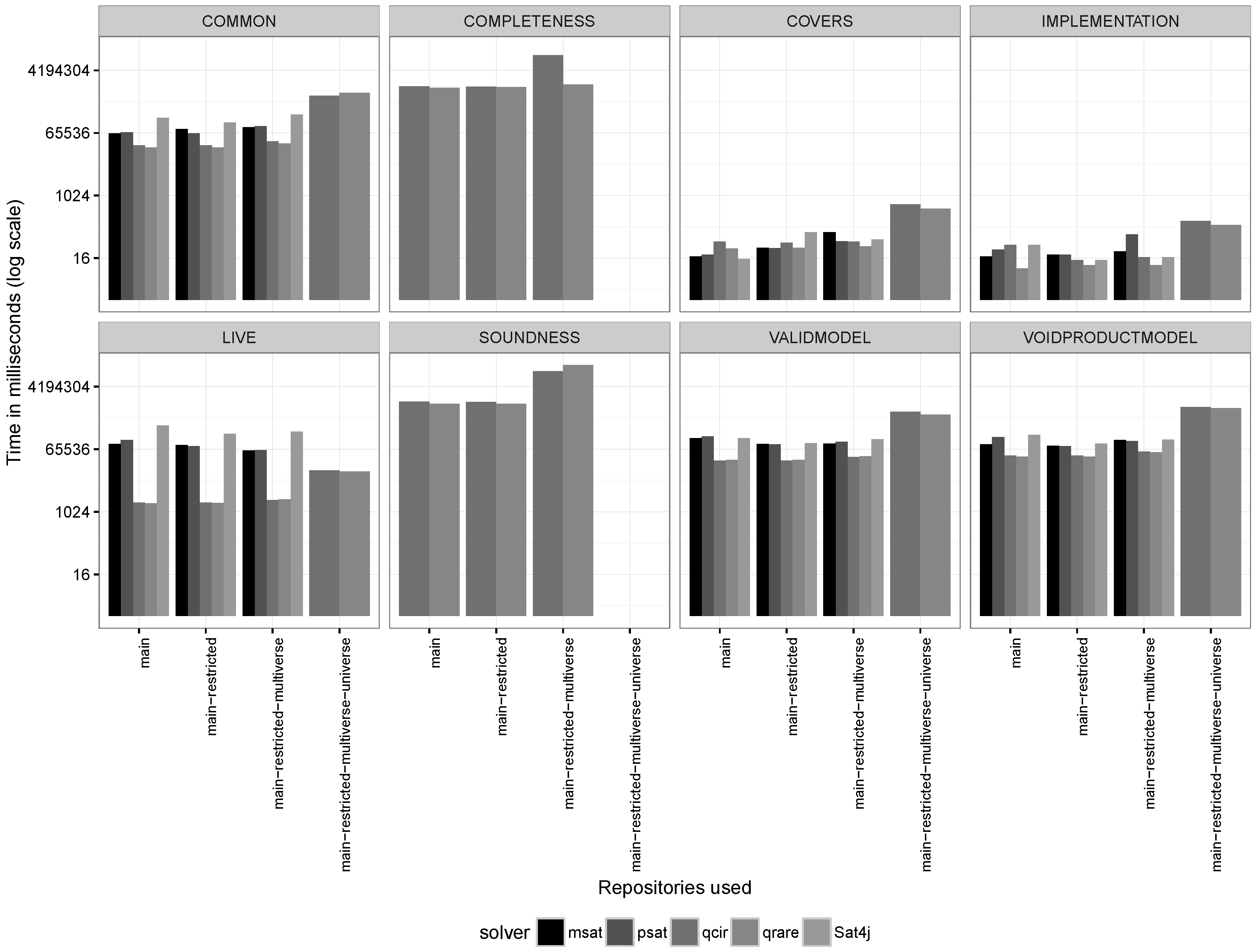
5.2.1. Experiment 1: Validating SPLAnE with Feature Models from the SPLOT Repository

To illustrate the SPL analysis method described in the paper, we considered case studies of various sizes. Concretely, the following SPLs were used: Entry Control Product Line (ECPL), Virtual Machine Product Line (VMPL), Mobile Phone Product Line (MPPL), Tablet Product Line (TPL) and Electronic Shopping Product Line (ESPL). The TPL, MPPL, and ESPL models were taken from the SPLOT repository [41]. More details of the ECPL models can be found at [26].

Table 4. Time complexity for properties and formulae with SPLAnE reasoner: CirQit. (# means the “Number” of features and components.)

SPL name	ECPL	VMPL	MPPL	TPL	ESPL
#Features	8	15	25	34	290
#Components	12	20	41	40	290
Analysis Operations	Time (ms)	Time (ms)	Time (ms)	Time (ms)	Time (ms)
$ValidFeatureModel$	10	14	14	20	35
$ValidComponentModel$	12	15	13	12	37
$ValidSPLModel$	14	16	15	28	40
$VoidProductModel$	18	25	23	29	55
$ValidSpecification$	7	13	11	17	45
$ValidImplementation$	9	15	13	12	48
$Complete$$Traceability$	0	1	0	1	1
$Implements$	8	10	9	10	22
$Realizes$	10	26	24	14	78
$Covers$	12	13	10	14	74
$Completeness$	18	30	26	284	2135
$Soundness$	350	2120	1323	730	6550
$Common$	15	22	19	28	74
$Live$	18	45	61	25	82
$Dead$	11	20	18	27	65
$Redundant$	14	24	19	21	38
$Critical$	10	14	15	19	34
$UnionoverSpecifications$	14	18	16	26	45
$UnionoverImplementations$	18	30	25	35	37
$UnionoverProducts$	18	24	20	32	48
$IntersectionoverSpecifications$	9	14	11	22	37
$IntersectionoverImplementations$	11	17	16	28	28
$IntersectionoverProducts$	15	20	21	19	46

gives the number of features, components in each SPL model, and the execution time taken by various analysis operations on SPLAnE reasoner: CirQit.

The SPLOT repository is a common place where a practitioners store feature models for the sake of reuse and communication. The SPLOT repository contains small and medium size feature models, most of it are conceptual and few are realistic. We extracted 698 feature models from the SPLOT repository. These feature models were given as an input to extended Betty tool to generate corresponding SPL models. Usually, components models which represent the solution space of SPLs are larger in size. So, the generated component models contain three-times more components then the number of features present in the corresponding feature model. SPLAnE generated the random traceability relation between feature model and component model to generate a complete SPL model. Further, to increase the complexity of experiments, each SPL model is generated using 10 different topologies and 10 different level of cross-tree constraints with percentage as $\{5,10,15,20,25,30,35,40,45,50\}$, resulting in a total of 100 SPL models per SPLOT model. So from 698 SPLOT models, we got 69800 SPL models. The percentage of cross-tree constraint is defined by the percentage of constraints over the number of features. Basically it is the number of constraints depending on the number of features. For example, if we specify a 50% percentage over a model with 10 features, then we have five cross-tree constraints.

The tool SPLAnE was executed with 69800 SPL models to verify the QSAT scalability when applying it to feature modeling. SPLAnE provide an option to select any one of the two QSAT reasoners (CirQit and RaReQS). Figure 5 shows the box plot, representing the QSAT behavior with increase in cross-tree constraints for few analysis operations on real models taken from the SPLOT repository. This experiment was executed with the QSAT reasoner CirQit. The results for experiment 1 (Section 5.2.1) shows that for the small and medium size real models, all analysis operations does not take much execution time which motivated us to experiments with large size models. The overall results for experiment 1 (Section 5.2.1) point out that the null hypothesis $H_0$ was wrong, thus, resulting in the acceptance of the alternative hypothesis $H_1$.

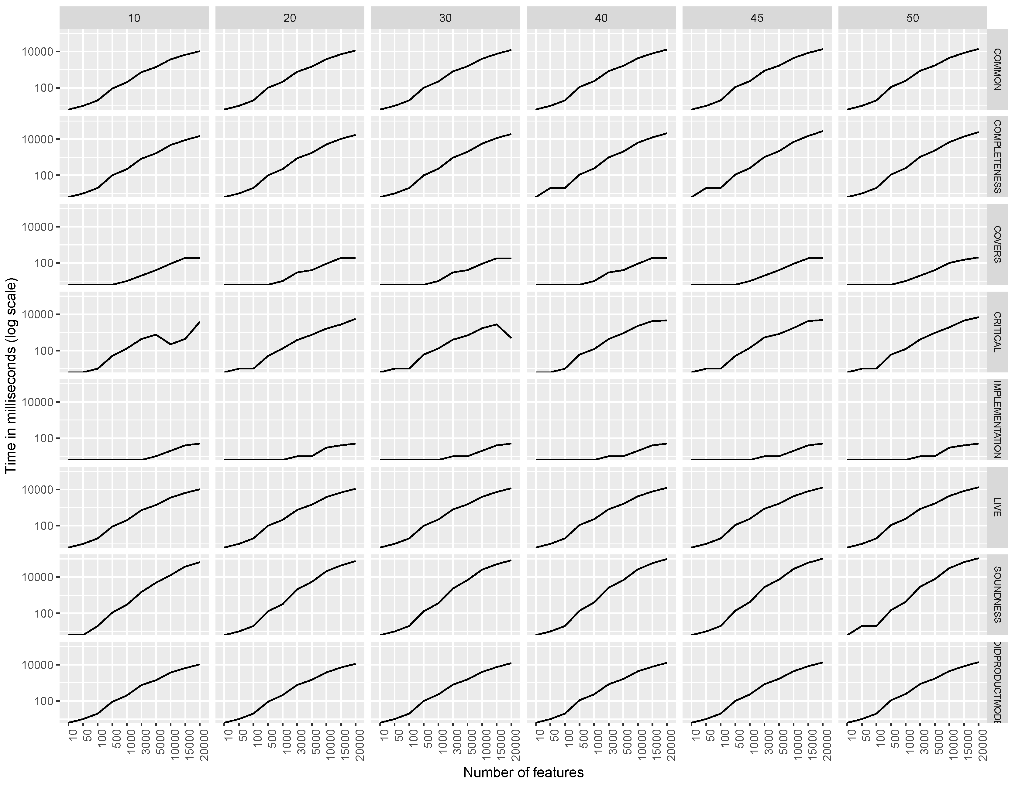
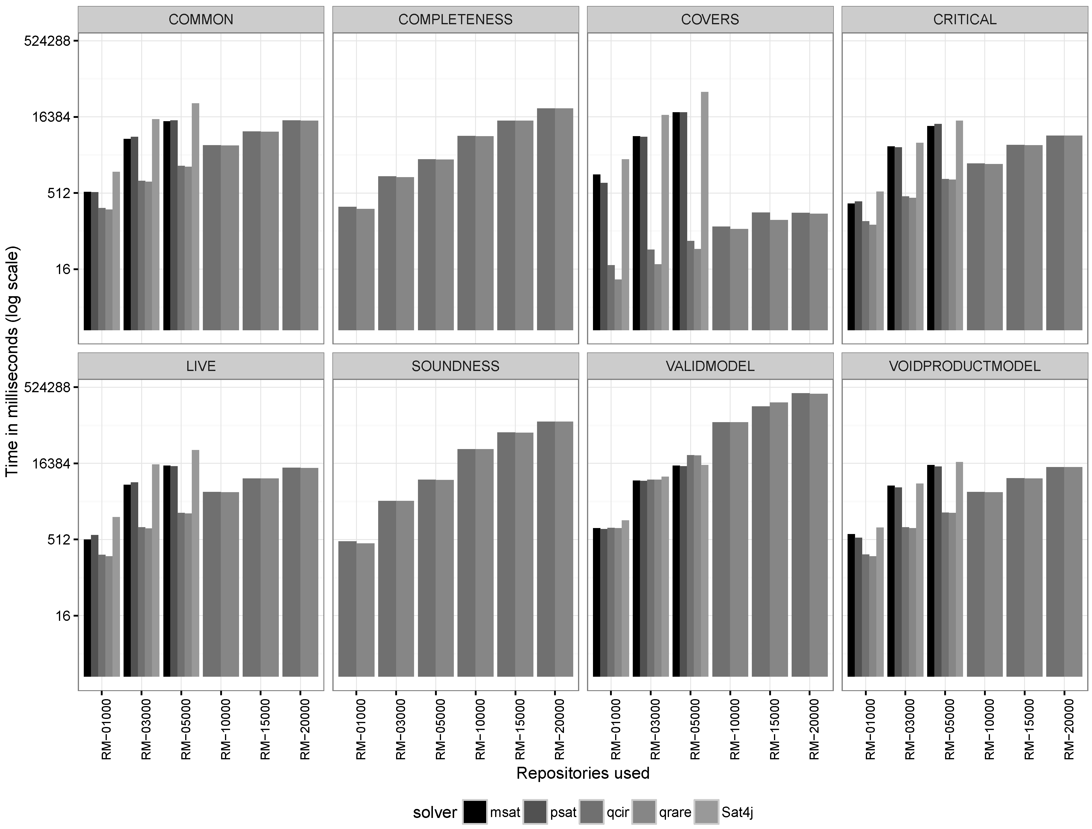
5.2.2. Experiment 2: Validating SPLAnE with Randomly Generated Large Size SPL Models

In this experiment we have compared scalability of SPLAnE and FaMa based analysis techniques over a large size randomly generated SPL models. The Betty tool suite [42] is used to generate random feature models relying on the approach of Thüm et al. [43]. SPLAnE extended the Betty tool suite to generate a set of random SPL models. Those models were generated for a number of features ranging from ten features to twenty thousand features. Concretely, $\{10,50,100,500,1000,3000,5000,10,000,15,000,20,000\}$ features with three-times larger size of each component models. For each SPL model, 10 different topologies were generated to avoid the threats to internal validity. Further, to increase the complexity of experiments, 10 different levels of cross-tree constraints $\{5,10,15,20,25,30,35,40,45,50\}$ were added. Each randomly generated SPL models consists of a feature model, a component model and a traceability relation. Note that, for model with 20,000 features there are 60,000 components in component model, which result in 80,000 variables in a generated SPL model. For each model, 10 different topologies and 10 levels of cross-tree constraints will result in 100 random SPL models, so in total 1000 SPL model were generated. The tool SPLAnE was executed against randomly generated 1000 SPL models to check the scalability of our approach with all analysis operations. Figure 6 shows the box plot for randomly generated large size SPL models. For data clarity we plotted only eight analysis operations for all models (except models with 50 features) and $\{10,20,30,40,50\}$ cross-tree levels of constraints. The experiment 2 (Section 5.2.2 was executed with SPLAnE reasoner: RaReQS. The plot clearly shows the QSAT approach is more scalable even with 80,000 variables in a SPL model with maximum 50% constraints. The Figure 6 show that the execution time for all analysis operation grows with the increase in number of features. Figure 7 shows the graph plot for the same results, which help to clearly distinguish the behavior of each analysis operations against the Cross Tree Constraints (CTC) levels. From the graphs we observed that, the number of features in a model has more impact on the execution time than the different levels of CTC. The levels of CTC has very less impact on the execution time. The operation soundness take more time as it check for all implementations there exist a specification and the number of components are three times more than the number of features. The operation completeness take less time as compared to soundness, but take more time compared to all remaining operations. In completeness we check for all specifications there exist an implementation, here the number of features are less compared to the number of components. So the completeness requires less execution time compare to soundness. The results for experiments 2 (Section 5.2.2) shows that, SPLAnE can scale up to 80,000 variables size models and this rule out the hypothesis $H_0$ with no option to accept the alternative hypothesis $H_1$.

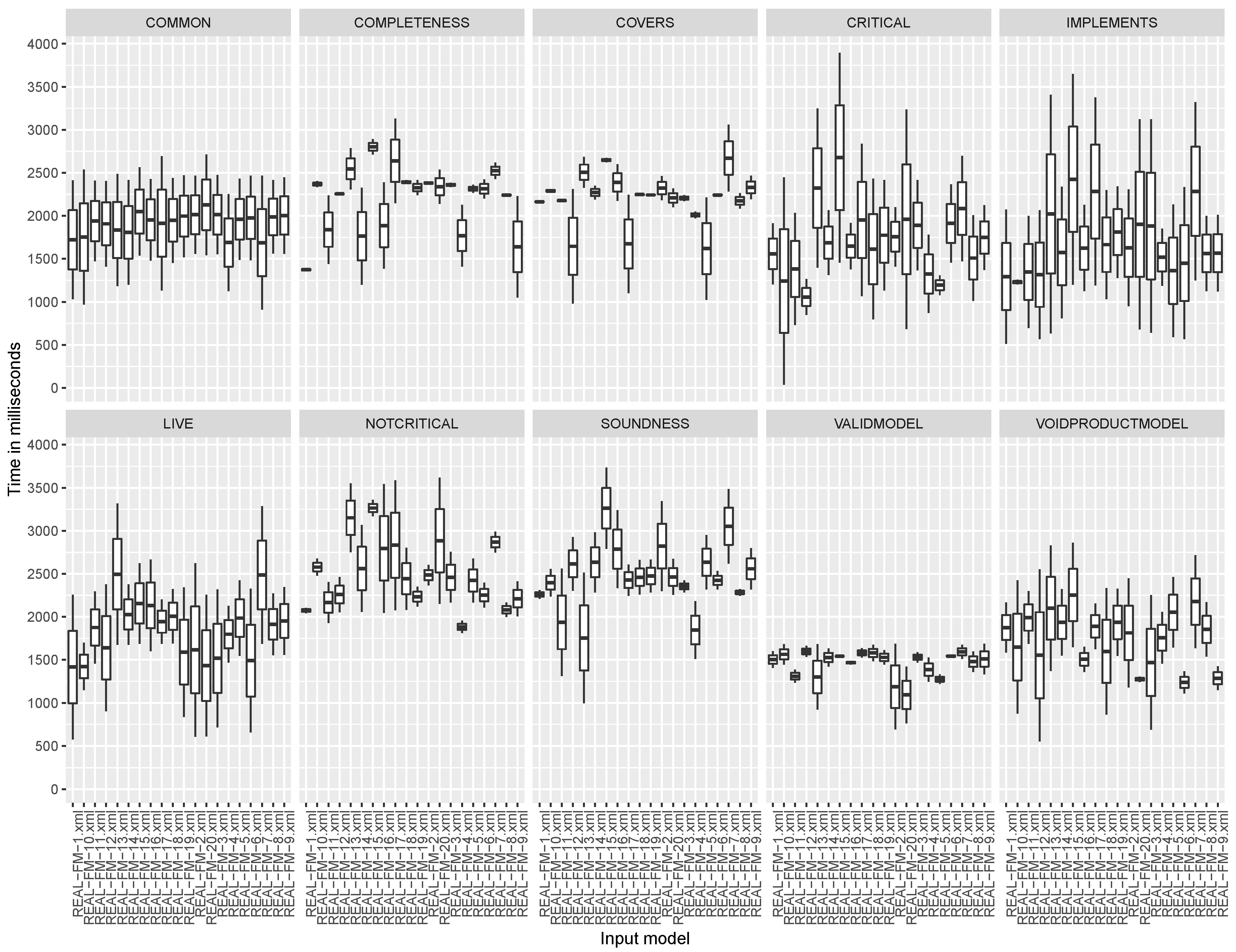
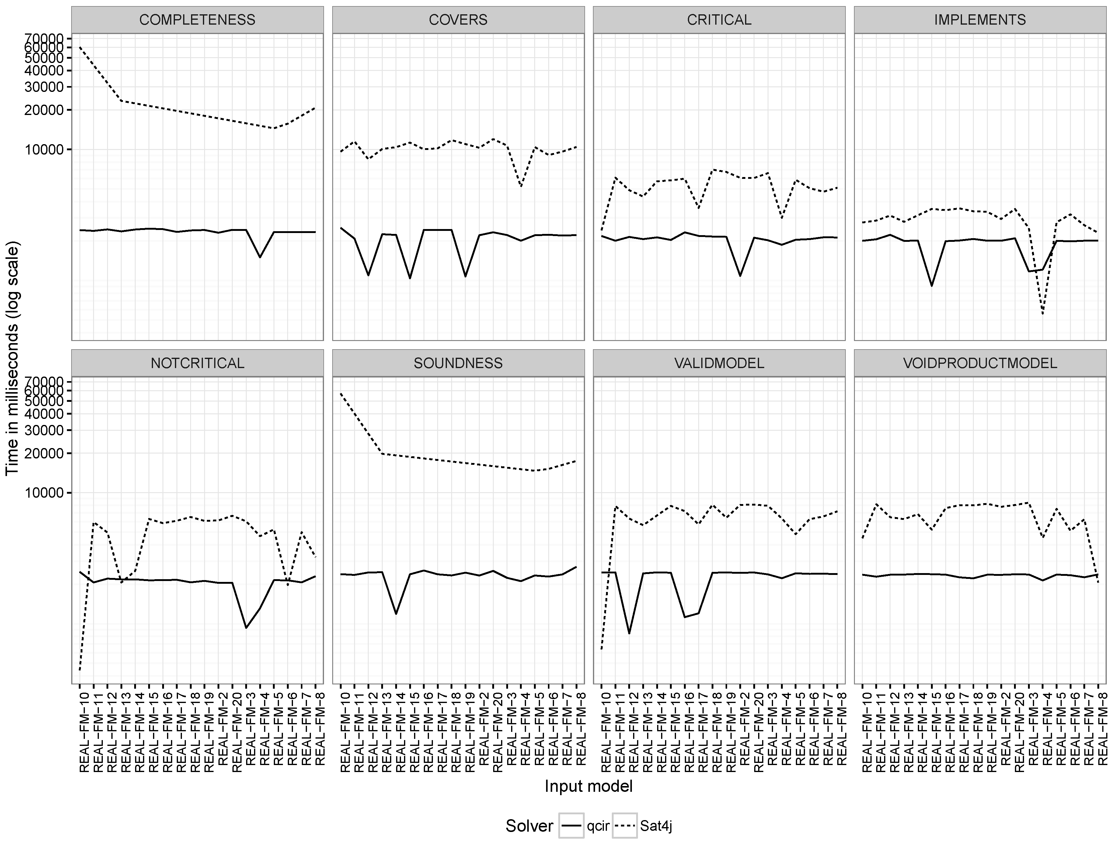
5.2.3. Experiment 3: Comparing SPLAnE and FaMa Approach in Front of Real and Large Debian Models

This experiment checks the behavior of SPLAnE reasoners (CirQit and RaReQS) and FaMa reasoners (Sat4j, PicoSAT and MiniSAT) on real and large Debian models with the analysis operation presented in the paper. We used the feature model extracted from Debian distributions [37]. This model encodes the variability present in the Ubuntu 10.04 distribution packaging system. We used four initial models containing the data from the repositories: main (7065 features), restricted (7098 features), multiverse (8122 features) and universe (26,338 features). To generate the SPL model from this real feature model, we used the same actual models as component models and linked each feature with component by naming with require relationships doubling than the number of variables within the model. Consider, the universe Debian model with 26,338 features then its corresponding SPL model will contain 52,676 variables.

Figure 8 shows the performance of SPLAnE reasoners (CirQit and RaReQS) and FaMa reasoners (Sat4j, PicoSAT and MiniSAT) against the proposed analysis operations. We see that both approaches scale for all operations in first three Debian models except the completeness and soundness where QSAT is clearly more efficient. For completeness and soundness operations, FaMa reasoners was not able to solve even a single instance of the Debian models. For the fourth model, i.e., universe Debian model, FaMa reasoners was not able to solve any of the analysis operations. Whereas QSAT reasoners against completeness and soundness operations, was able to solve first three Debian models (main, restricted, multiverse), but was not able to solve the huge universe Debian model (26,338 features) in the given timeout (two hours). Overall, for the operations where both approaches scale up, QSAT is faster than SAT. This experiments clearly accepts the hypothesis $H_1$.

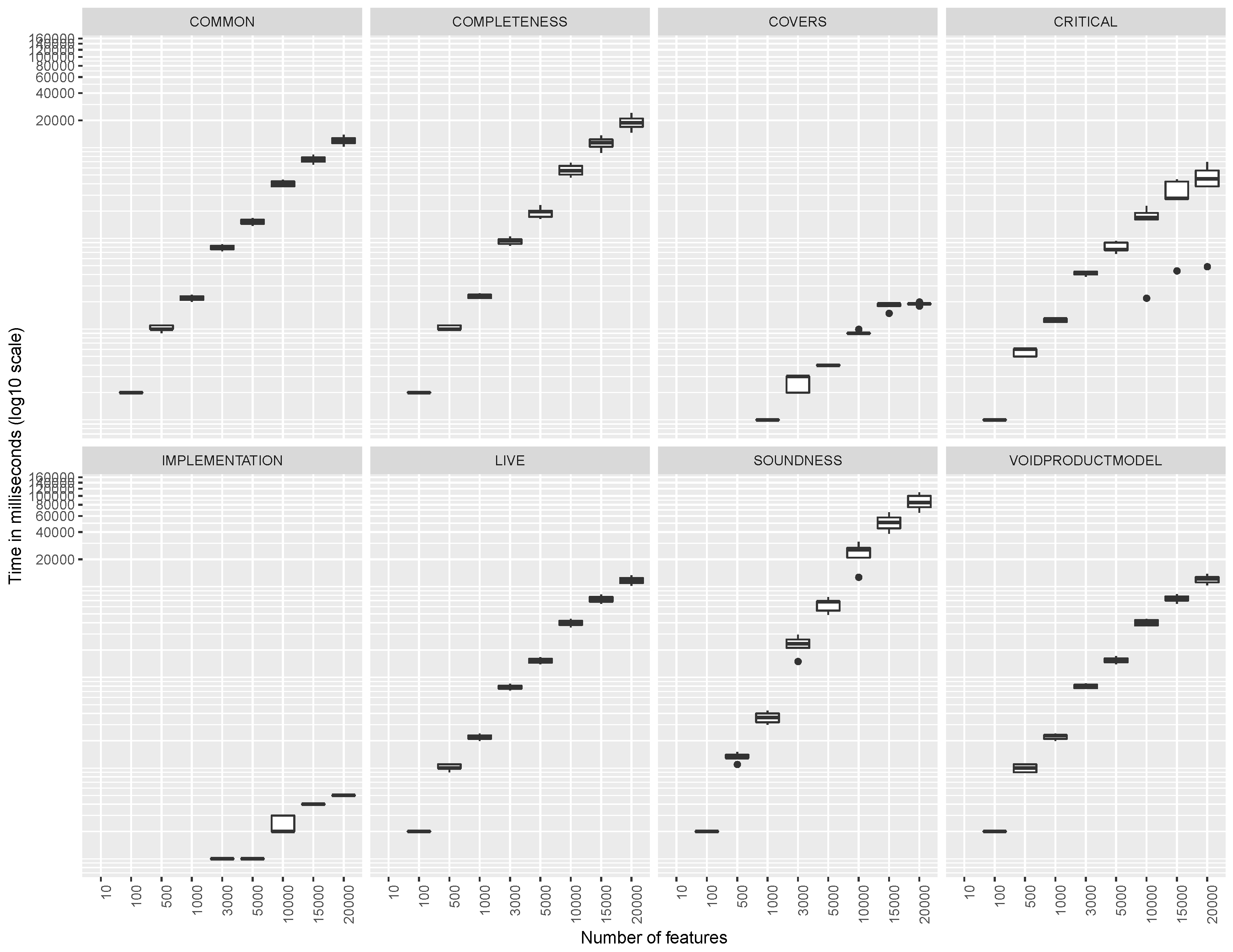
5.2.4. Experiment 4: Comparing SPLAnE and FaMa Scalability in Front of Randomly Generated Large Size Models

In this experiment, we checked the behavior of SPLAnE reasoners (CirQit and RaReQS) and FaMa reasoners (Sat4j, PicoSAT and MiniSAT) on randomly generated SPL models taken from experiments 2 (Section 5.2.2). Figure 9 shows the scalability of SPLAnE reasoners and FaMa reasoners against randomly generated models. The results are only shown for large models from 1000 features to 20,000 features with 50% cross-tree constraints. Here, the feature model with 10,000 features means its corresponding SPL model contains 40,000 variables with 50% CTC. The results clearly shows that, the SAT reasoners are not able to solve any analysis operations after getting a models of size 10,000 features or more. For completeness and soundness operations, SAT reasoners was not able to solve any SPL models after 1000 features. The QSAT reasoners were able to solve all analysis operations on the random SPL models. The results deny the hypothesis $H_0$ with an option left to accept the hypothesis $H_1$.

5.2.5. Experiment 5: Comparing SPLAnE with FaMa based Reasoning Techniques

The tool SPLAnE improves the performance with the set of models obtained from SPLOT and random SPL models. In this experiment, we are comparing QSAT based technique with SAT based techniques over the analysis operations. From the SPLOT models used in the experiment 1 (Section 5.2.1) we took those marked as realistic. FaMa supports analysis operations expressed using propositional formulae. We acknowledge that there are analysis operations such as completeness and soundness that cannot be expressed using propositional formulae. So, for comparing QSAT vs. SAT reasoning, such operations where written in the FaMa tool suite with loop statements (for or while) for traversing the whole set of solutions. Here, the loop allows us to express such operations (completeness, soundness, etc.) to its equivalent QSAT formula but note that, the complete operations cannot be expressed using standalone propositional formula. Later, we executed the analysis operations with SPLAnE reasoner (CirQit and the FaMa reasoner) Sat4j.

Figure 10 shows the results for QSAT vs. SAT based reasoning for few analysis operations on real models taken from the SPLOT repository. QSAT defeat SAT encoded formulae for every analysis operations. The execution of all models is available on website at [44] as well as the scripts used to generate this data. The first noticeable results are that SPLAnE overtakes all executions of all operations when comparing to the standard FaMa version (which is using Sat4j as a solver). Moreover, we see improvements of more than 70% (note the log scale) when talking about the soundness operation. Therefore, after trying to refute the null hypothesis $H_0$ (for experiment 5 (Section 5.2.5)) with no luck, we have to accept the alternative hypothesis $H_1$ which states that SPLAnE is faster and scalable than previously standard SAT-based techniques.

5.3. Threats to Validity

Even though the experiments presented in this paper provide evidence that the solution proposed is valid, there are some conditions that may affect their validity. In this section, we discuss the different threats to validity that affect the evaluation.

External Validity: The inputs used for the experiments presented in this paper try to mimic realistic feature models. However, SPLOT models are not necessarily realistic. To ease off this threat we decide to used feature models based on the Debian repository. Furthermore, the random feature models may not reflect the same structure as other realistic models. The major threats to the external validity are:

• Population validity, the models may not be realistic. To reduce these threats, we generated the models as in [43] and implemented in the Betty tool [42]. We also, used model coming out the Debian repositories to provide more realistic topologies.
• Ecological validity: While external validity, in general comes with the generalization of the results to other contexts (e.g., using other models), the ecological validity faces the threats affecting the experiment materials and tools. To prevent the threats of third party threads running on the machines, SPLAnE analyses were executed 10 times and then averaged.

Internal validity: The CPU capabilities required when analyzing an SPL model depend on the number of features, components and percentage of cross-tree constraints. However, there might be some variables affecting the performance, such as the topology, so we generated 10 different topologies for each SPL model.

Construct validity: The results look promising in terms of time required to solve problems related to the feature model. However, we can not grant its validity with models more than 20,000 features.

6. Related Work

Automated Analysis of Feature Models. The automated analysis of feature models has been around for more than 20 years [6]. Up to 30 different analysis operations have been presented. However, there is a lack of support for implementation assets and their relations with the variability management. In this paper, we extend the variability management analysis with the automated analysis of feature models among the implementation of the different features. White et al. [45] presented an approach to automate the configuration in SPLs by transforming feature model and configurations in Constraint Satisfaction Problem (CSP). The CSP are used to diagnose errors in the selected features. In the case of invalid configuration, it repairs the selected features. Authors also verified their approach on the feature models in the rang of 100 to 5000 features. Bagheri et al. shows the approach to construct feature models with its constraints using a propositional formulae [46]. They also explained the formalism to configure a semi-automated feature model. Soltani et al. gives the configurations process based on artificial intelligence planning technique to derive product from a feature model automatically according to the stakeholders requirements, were the stakeholders may have diverse business and limited resources [47].

Traceability in SPLs. While there is a fairly large body of work in the literature on different facets of SPL, in the following we mention only those which address traceability as a primary aspect. Four important characteristics of a variability model, namely, consistency, visualization, scalability and traceability are defined in [9]. A variability management model that focuses on the traceability aspect of the notion of problem and solution spaces is presented in [2]. Anquetil et al. [8] formalize the traceability relations across the problem and solution space and also across domain and product engineering. In [12], the notion of product maps is defined which is a matrix giving the relation between features and products. Consistency analysis of product maps is presented in [13]. Zhu et al. [15] define a traceability relation from requirements to features and also from features to architectures, with consistency analysis. Reference [14] lpresents a method to identify the traceability between feature model and architecture model. The Czarnecki’s work [3,10,11] on giving semantics to features in feature models by mapping them to other models has been found useful at the requirements level. However, none of the works mentioned above present the formal approach for analyses operations, nor it address the role of traceability in the implementability aspect of SPLs.

Implementation derivation. Borba et al. [48] build on the idea of automatic generation of products from assets by relying on feature diagrams and configuration knowledge (CK) [3]. A CK relates features to assets specifying that assets implement possible feature combinations. The reference [48] lays theoretical foundations on refining and evolving SPLs. The notion of traceability in [48] is general; however, unlike the reference [48], the focus of our paper is on the implementability of SPLs.

Template-based traceability. In [10,11], the authors propose a template-based approach for mapping feature models to annotated models expressed in Unified Modeling Language (UML) or a domain-specific modeling language. Based on a particular configuration of features, an instance of the template is created by evaluating presence conditions in the model. The reference [11] gives a verification procedure which establishes that no ill-formed template instances will be produced given a correct configuration of the feature model. The procedure takes a feature model and an annotated template, which is an instance of a class model (like UML) and a set of OCL (Object Constraint Language) rules. The rules are written with respect to the class model, and each OCL constraint is an invariant on some class c. The final verification is done by checking the validity of a propositional formula. Our notion of traceability is more general than instantiating a template based on the presence of a set of features; moreover, our analysis operations require an encoding into QSAT and we have experimental evidence to suggest that the QSAT encoding performs well over SAT-based procedures (Figure 10).

Variability Management. The paper that is the closest to our work is that by Metzger et al. [20] and deserves a detailed comparison. In this paper, PL variability refers to the variations in the features of the system and software variability refers to the variations among the software system artifacts. In our paper, we follow a different terminology to bring out the product line hierarchy clearly (shown in Figure 11): a scope consists of all the features, a variant specification (referred to as just “specification”) is a subset of features, product line specification (PL specification) is a set of variant specifications. On the other hand, core assets comprise all the components, a variant implementation (referred to as just “implementation”) is a subset of components, product line implementation (PL implementation) is a set of variant implementations. The PL variability of Metzger et al. is analogous to PL specifications and software variability is analogous to PL implementations. In Metzger et al., PL variability is represented as OVM (Orthogonal Variability Model) and software variability is represented as FD (Feature Diagrams). In our paper, we give set-theoretic semantics to SPLs in lieu of the visually appealing notations such as FD, VFD and OVM. The advantage is that in these semantics the core concepts, analysis problems, and the solution methods can be expressed in a clearer and more concise manner.

The traceability among PL and software variability is represented in Metzger et al. using X-links. One type of X-links is of the form $f\iff V_1\vee V_2\vee \vee \cdots V_n$ which says a feature f is present iff at least one of the variations $V_i$ is present in the software variability. However, it cannot capture the fact that a feature may be implemented by different sets of software artifacts which may require constraints of the form $f\iff (c_{11}\wedge c_{12}\wedge c_{13})\vee (c_{21}\wedge c_{22}\cdots )\vee \cdots$. The other type of traceability constraints suggested in Metzger et al. is simple propositional formulae. However, not all propositional constraints provide the intuitive and strong implementability relations between the implementations and specifications. The definition of traceability in our paper captures the above-mentioned class of constraints and is used to define a reasonable notion of a relation between implementations and specifications.

Marcilio et al. presented the experimental results to prove the SAT-based approach to analyze a variability models like feature model is easy [49]. Authors have used feature models with maximum of 10,000 feature. To increase the hardness, feature models where added with 10%, 20% and 30% of cross-tree constraints (CTC). They found that realistic feature models are not difficult for SAT solvers.

Steven et al. present the heuristic to generate a feature model from an existing system using reverse engineering [50]. They used three real system as Linux, eCos and FreeBSD. The Linux has a variability model represented by Kconfig Language and eCos has Component Definition Language, where as FreeBSD has a list of features. The approach was able to successfully generate the feature model from Linux, eCos and FreeBSD systems.

Mikolás et al. presents a meta model which is mechanically formalized from the feature models in the literature [51]. This meta model is used for feature modeling and reasoning about it. Larger size SPLs development involves manipulating many parts in FMs. The paper [52] propose an compositional approach to develop complex SPLs with the help of complimentary operators like aggregate, merge and slice. Along with reasoning, the paper present methods for correction of anomalies, update and extraction and reconciliation of FMs.

The SAT-based definition of products in Metzger et al. allows causally unrelated components and features as products of the SPL. At other times, it is too restrictive in that it does not allow additional components in an implementation which do not provide any feature, but are forced to be with other components because of, say, packaging restrictions. It seems necessary to strike the right balance between the strictness of X-links and the general propositional constraints for a reasonable definition of implementability. This is provided by the definition of the relation $Covers$ in our paper.

Metzger et al. propose a number of analysis problems; in the terminology of that paper, they are realizability, internal competition, usefulness, flexibility and common and dead elements. We have redefined these in our paper from the perspective of the new implements relation. Moreover, we have described some new and useful SPL analysis problems (superfluous, redundancy, critical component, extraneous features). In Metzger et al., it was noted that the satisfiability-based formulation needed to enumerate and check all the implementations and specifications in order to solve certain analysis problems. Hence, the cumulative complexity of satisfiability checking may be prohibitive for large SPLs. The QSAT based formulation proposed in our paper obviates this problem and gives efficient solution methods scalable to large, real-life case studies. Figure 10 gives a comparison of SAT and QSAT approaches for the analysis operation soundness and completeness. The time complexity shown in the figure shows the superiority of the QSAT approach over SAT-based approaches for some analysis problems. On a bigger case study (ESPL in Section 5), which had 290 features and an equal number of components, the SAT-based approach failed to solve any of the analysis problems.

7. Future Work

In future work, we plan to focus on the following extension aspects of this paper:

• More solvers: Currently, we have implemented SPLANE analysis operations using a reduced number of QSAT and SAT solvers. In the future we plan to add some SMT (Satisfiability Modulo Theories) solvers to this list and proceed with comparative study detecting the pros and cons of each approach.
• Granularity: In this paper we have considered that the traceability relation exists at the level of features and components. However, A traceability relation can be extended to map a feature with a part of components or a component can be decompose into sub-component to perform a granular mapping or multi-level mapping.
• Logic paradigms: We have focused on SAT solving techniques, however, there are some other approaches such as BDD that are appealing for the same usage. In the future, we plan to do a comparison between a QSAT approach presented in paper and quantification over BDD with the implementation across all the analysis operation.
• Experimentation: In this paper, we have evaluated our approach in a diverse set of scenarios however, we focused in examples containing only 1:m relationships. In the future work we plan to extend the experimentation to n:m relationships to see if this has implications in the scalability of our solution.

8. Conclusions

In this paper, we stress the need to jointly analyze the specification and the implementation of SPLs. Thus, we have started from a formal definition of the notion of traceability and a set theoretical-based framework. We imported existing analyses and propose new analyses, such as superfluousness, explicitness, redundant, union, intersection, valid model, void product model, complete traceability, etc. The analysis problems have been translated into Quantified Boolean Formula and solved efficiently using a QBF solver. The approach is supported by a software tool called SPLAnE and integrated with the existing FaMa framework. We conducted a detailed experimentation with SPLAnE on: (i) large Debian models; (ii) randomly-generated models; and (iii) SPLOT models. We executed all analysis operations with five solvers, i.e., two QSAT solvers (CirQit and RaReQS) and three SAT solvers (Sat4j, PicoSAT and MiniSAT). Further, we experimented SPLAnE for scalability. The experiments are also conducted on the QSAT approach vs. the SAT approach. For scalability, we took the extended Betty tool and generated a random set of SPL models ranging from five to 50 percent of cross-tree constraints, with 10 different topology and from 10 features to 20,000 features. The scalability result shows that the tool SPLAnE was able to analyze such huge SPL models. The comparison between SAT vs. QSAT results clearly shows that our approach improved the performance by 70% over the SAT-based approach for the analysis operations, like soundness and completeness.

References

1. Czarnecki, K.; Wasowski, A. Feature diagrams and logics: There and back again. In Proceedings of the 11th International Software Product Line Conference (SPLC 2007), Kyoto, Japan, 10–14 September 2007; pp. 23–34.
2. Berg, K.; Bishop, J.; Muthig, D. Tracing software product line variability: From problem to solution space. In Proceedings of the 2005 Annual Research Conference of the South African Institute of Computer Scientists and Information Technologists on IT Research in Developing Countries, White River, South Africa, 20–22 September 2005; pp. 182–191.
3. Czarnecki, K.; Eisenecker, U.W. Generative Programming: Methods, Tools, and Applications; Addison-Wesley Publishing: New York, NY, USA, 2000. [Google Scholar]
4. Pohl, K.; Böckle, G.; van der Linden, F.J. Software Product Line Engineering—Foundations, Principles, and Techniques; Springer: Berlin/Heidelberg, Germany, 2005. [Google Scholar]
5. Clements, P.C.; Northrop, L.M. Software Product Lines: Practices and Patterns; Addison-Wesley: Boston, MA, USA, 2001. [Google Scholar]
6. Benavides, D.; Segura, S.; Cortés, A.R. Automated analysis of feature models 20 years later: A literature review. Inf. Syst. 2010, 35, 615–636. [Google Scholar] [CrossRef] [Green Version]
7. Pohl, K.; Metzger, A. Variability management in software product line engineering. In Proceedings of the 28th International Conference on Software Engineering, Shanghai, China, 20–28 May 2006; ACM: New York, NY, USA, 2006; pp. 1049–1050. [Google Scholar]
8. Anquetil, N.; Grammel, B.; Galvao Lourenco da Silva, I.; Noppen, J.A.R.; Shakil Khan, S.; Arboleda, H.; Rashid, A.; Garcia, A. Traceability for model driven, software product line engineering. In Proceedings of the ECMDA Traceability Workshop, Berlin, Germany, 12 June 2008; pp. 77–86.
9. Beuche, D.; Papajewski, H.; Schröder-Preikschat, W. Variability management with feature models. Sci. Comput. Program. 2004, 53, 333–352. [Google Scholar] [CrossRef]
10. Czarnecki, K.; Antkiewicz, M. Mapping features to models: A template approach based on superimposed variants. In Proceedings of the 4th International Conference on Generative Programming and Component Engineering, Tallinn, Estonia, 29 September–1 October 2005; Springer: Berlin/Heidelberg, Germany, 2005; pp. 422–437. [Google Scholar]
11. Czarnecki, K.; Pietroszek, K. Verifying feature-based model templates against well-formedness OCL constraints. In Proceedings of the 5th International Conference on Generative Programming and Component Engineering, Portland, OR, USA, 22–26 October 2006; ACM: New York, NY, USA, 2006; pp. 211–220. [Google Scholar]
12. DeBaud, J.M.; Schmid, K. A systematic approach to derive the scope of software product lines. In Proceedings of the 21st International Conference on Software Engineering, Los Angeles, CA, USA, 16–22 May 1999; ACM: New York, NY, USA, 1999; pp. 34–43. [Google Scholar]
13. Eisenbarth, T.; Koschke, R.; Simon, D. A formal method for the analysis of product maps. In Proceedings of the Requirements Engineering for Product Lines Workshop, Essen, Germany, 9–13 September 2002.
14. Satyananda, T.K.; Lee, D.; Kang, S.; Hashmi, S.I. Identifying traceability between feature model and software architecture in software product line using formal concept analysis. In Proceedings of the International Conference on Computational Science and its Applications (ICCSA 2007), Kuala Lumpur, Malaysia, 26–29 August 2007; pp. 380–388.
15. Zhu, C.; Lee, Y.; Zhao, W.; Zhang, J. A feature oriented approach to mapping from domain requirements to product line architecture. In Proceedings of the 2006 International Conference on Software Engineering Research and Practice, Las Vegas, NV, USA, 26–29 June 2006; pp. 219–225.
16. Anquetil, N.; Kulesza, U.; Mitschke, R.; Moreira, A.; Royer, J.C.; Rummler, A.; Sousa, A. A model-driven traceability framework for software product lines. Softw. Syst. Model. 2010, 9, 427–451. [Google Scholar] [CrossRef] [Green Version]
17. Cavalcanti, Y.A.C.; do Carmo Machado, I.; da Mota, P.A.; Neto, S.; Lobato, L.L.; de Almeida, E.S.; de Lemos Meira, S.R. Towards Metamodel Support for Variability and Traceability in Software Product Lines. In Proceedings of the 5th Workshop on Variability Modeling of Software-Intensive Systems, Namur, Belgium, 27–29 January 2011; ACM: New York, NY, USA, 2011; pp. 49–57. [Google Scholar]
18. Ghanam, Y.; Maurer, F. Extreme product line engineering: Managing variability and traceability via executable specifications. In Proceedings of the 2009 Agile Conference, Chicago, IL, USA, 24–28 August 2009; pp. 41–48.
19. Riebisch, M.; Brcina, R. Optimizing design for variability using traceability links. In Proceedings of the 15th Annual IEEE International Conference and Workshop on the Engineering of Computer Based Systems, Belfast, Northern Ireland, 31 March–4 April 2008; IEEE: Washington, DC, USA, 2008; pp. 235–244. [Google Scholar]
20. Metzger, A.; Heymans, P.; Pohl, K.; Schobbens, P.Y.; Saval, G. Disambiguating the documentation of variability in software product lines: A separation of concerns, formalization and automated analysis. In Proceedings of the 15th IEEE International Requirements Engineering Conference (RE 2007), Delhi, India, 15–19 October 2007; pp. 243–253.
21. SAT4J-Solver. Available online: http://www.sat4j.org/ (accessed on 7 July 2016).
22. MiniSAT-Solver. Available online: http://minisat.se/ (accessed on 7 July 2016).
23. PicoSAT. Available online: http://fmv.jku.at/picosat/ (accessed on 7 July 2016).
24. CirQit. Available online: http://www.cs.utoronto.ca/~alexia/cirqit/ (accessed on 7 July 2016).
25. RAReQS-NN. Available online: http://sat.inesc-id.pt/~mikolas/sw/rareqs-nn/ (accessed on 7 July 2016).
26. Mohalik, S.; Ramesh, S.; Millo, J.V.; Krishna, S.N.; Narwane, G.K. Tracing SPLs precisely and efficiently. In Proceedings of the 16th International Software Product Line Conference–Volume 1, Salvador, Brazil, 2–7 September 2012; pp. 186–195.
27. Benavides, D.; Segura, S.; Trinidad, P.; Cortés, A.R. FAMA: Tooling a framework for the automated analysis of feature models. In Proceedings of the First International Workshop on Variability Modelling of Softwareintensive Systems, Limerick, Ireland, 16–18 January 2007; pp. 129–134.
28. SPLAnE. Available online: http://www.cse.iitb.ac.in/~splane/ (accessed on 7 July 2016).
29. Kang, K.C.; Cohen, S.G.; Hess, J.A.; Novak, W.E.; Peterson, A.S. Feature-Oriented Domain Analysis (FODA) Feasibility Study; Technical Report CMU/SEI-90-TR-21; Software Engineering Institute of Carnegie Mellon University: Pittsburgh, PA, USA, 1990. [Google Scholar]
30. Schobbens, P.Y.; Heymans, P.; Trigaux, J.C.; Bontemps, Y. Generic semantics of feature diagrams. Comput. Netw. 2007, 51, 456–479. [Google Scholar] [CrossRef]
31. Batory, D. Feature models, grammars, and propositional formulas. In Proceedings of the 9th International Conference on Software Product Lines, Rennes, France, 26–29 September 2005; pp. 7–20.
32. The Yices SMT Solver. Available online: http://yices.csl.sri.com/ (accessed on 7 July 2016).
33. BDDSolve. Available online: http://www.win.tue.nl/~wieger/bddsolve/ (accessed on 7 July 2016).
34. Stockmeyer, L.J. The polynomial-time hierarchy. Theor. Comput. Sci. 1976, 3, 1–22. [Google Scholar] [CrossRef]
35. SPLAnE-TR. Available online: http://www.cse.iitb.ac.in/~krishnas/tr2012.pdf (accessed on 7 July 2016).
36. Roos-Frantz, F.; Galindo, J.A.; Benavides, D.; Ruiz-Cortés, A. FaMa-OVM: A tool for the automated analysis of OVMs. In Proceedings of the 16th International Software Product Line Conference, Salvador, Brazil, 2–7 September 2012; pp. 250–254.
37. Galindo, J.A.; Benavides, D.; Segura, S. Debian packages repositories as software product line models. Towards automated analysis. In Proceedings of the 1st International Workshop on Automated Configuration and Tailoring of Applications, Antwerp, Belgium, 20 September 2010; pp. 29–34.
38. Seidl, M. The qpro Input Format: A Textual Syntax for QBFs in Negation Normal Form. Available online: http://qbf.satisfiability.org/gallery/qpro.pdf (accessed on 7 July 2016).
39. Gallery, Q. QCIR-G14: A Non-Prenex Non-CNF Format for Quantified Boolean Formulas. Available online: http://qbf.satisfiability.org/gallery/qcir-gallery14.pdf (accessed on 7 July 2016).
40. Peschiera, C.; Pulina, L.; Tacchella, A.; Bubeck, U.; Kullmann, O.; Lynce, I. The Seventh QBF Solvers Evaluation (QBFEVAL’10). In Proceedings of the 13th International Conference (SAT 2010), Edinburgh, UK, 11–14 July 2010; pp. 237–250.
41. Mendonca, M.; Branco, M.; Cowan, D. SPLOT: Software product lines online tools. In Proceedings of the 24th ACM SIGPLAN Conference Companion on Object Oriented Programming Systems Languages and Applications, Orlando, FL, USA, 25–29 October 2009; ACM: New York, NY, USA, 2009; pp. 761–762. [Google Scholar]
42. Segura, S.; Galindo, J.A.; Benavides, D.; Parejo, J.A.; Ruiz-Cortés, A. BeTTy: Benchmarking and testing on the automated analysis of feature models. In Proceedings of the Sixth International Workshop on Variability Modeling of Software-Intensive Systems, Leipzig, Germany, 25–27 January 2012; pp. 63–71.
43. Thüm, T.; Batory, D.S.; Kästner, C. Reasoning about edits to feature models. In Proceedings of the 31st International Conference on Software Engineering (ICSE 2009), Vancouver, BC, Canada, 16–24 May 2009; pp. 254–264.
44. SPLAnE. Available online: http://www.cse.iitb.ac.in\~splane (accessed on 7 July 2016).
45. White, J.; Benavides, D.; Schmidt, D.; Trinidad, P.; Dougherty, B.; Ruiz-Cortes, A. Automated diagnosis of feature model configurations. J. Syst. Softw. 2010, 83, 1094–1107. [Google Scholar] [CrossRef] [Green Version]
46. Bagheri, E.; di Noia, T.; Ragone, A.; Gasevic, D. Configuring software product line feature models based on stakeholders’ soft and hard requirements. In Proceedings of the 14th International Conference on Software Product Lines: Going Beyond, Jeju Island, Korea, 13–17 September 2010; pp. 16–31.
47. Soltani, S.; Asadi, M.; Hatala, M.; Gasević, D.; Bagheri, E. Automated planning for feature model configuration based on stakeholders’ business concerns. In Proceedings of the 26th IEEE/ACM International Conference on Automated Software Engineering, Lawrence, KS, USA, 6–10 November 2011; pp. 536–539.
48. Borba, P.; Teixeira, L.; Gheyi, R. A theory of software product line refinement. Theor. Comput. Sci. 2012, 455, 2–30. [Google Scholar] [CrossRef]
49. Mendonca, M.; Wasowski, A.; Czarnecki, K. SAT-based analysis of feature models is easy. In Proceedings of the 13th International Software Product Lines (SPLC 2009), San Francisco, CA, USA, 24–28 August 2009; pp. 231–240.
50. She, S.; Lotufo, R.; Berger, T.; Wasowski, A.; Czarnecki, K. Reverse engineering feature models. In Proceedings of the 33rd International Conference on Software Engineering (ICSE 2011), Waikiki, HI, USA, 21–28 May 2011; pp. 461–470.
51. Janota, M.; Kiniry, J. Reasoning about feature models in higher-order logic. In Proceedings of the 11th International Software Product Lines (SPLC 2007), Kyoto, Japan, 10–14 September 2007; pp. 13–22.
52. Acher, M.; Collet, P.; Lahire, P.; France, R.B. Separation of concerns in feature modeling: Support and applications. In Proceedings of the 11th International Conference on Aspect-Oriented Software Development (AOSD 2012), Potsdam, Germany, 25–30 March 2012; pp. 1–12.
Figure 1. Feature model: virtual machine.
Entropy 18 00269 g001
Figure 2. Component model: Linux virtual machine-based system.
Entropy 18 00269 g002
Figure 3. Preconfigured virtual machines.
Entropy 18 00269 g003
Figure 4. SPLAnE reasoning process.
Entropy 18 00269 g004
Figure 5. Impact on QSAT scalability on Real SPLOT models with the increment in Cross Tree Constraints (CTC) levels.
Entropy 18 00269 g005
Figure 6. Boxplot for QSAT scalability on large random SPL models with the increment in CTC levels.
Entropy 18 00269 g006
Figure 7. QSAT scalability on large random SPL models with the increment in CTC levels.
Entropy 18 00269 g007
Figure 8. SPLAnE required time vs. FaMarequired time in front of real and large Debian based feature models.
Entropy 18 00269 g008
Figure 9. SPLAnE required time vs. FaMa required time in front of random and large SPL models.
Entropy 18 00269 g009
Figure 10. SPLAnE required time vs. FaMa required time.
Entropy 18 00269 g010
Figure 11. Product line hierarchy.
Entropy 18 00269 g011