Nonparametric Denoising Methods Based on Contourlet Transform with Sharp Frequency Localization: Application to Low Exposure Time Electron Microscopy Images ^†

Abstract

Image denoising is a very important step in cryo-transmission electron microscopy (cryo-TEM) and the energy filtering TEM images before the 3D tomography reconstruction, as it addresses the problem of high noise in these images, that leads to a loss of the contained information. High noise levels contribute in particular to difficulties in the alignment required for 3D tomography reconstruction. This paper investigates the denoising of TEM images that are acquired with a very low exposure time, with the primary objectives of enhancing the quality of these low-exposure time TEM images and improving the alignment process. We propose denoising structures to combine multiple noisy copies of the TEM images. The structures are based on Bayesian estimation in the transform domains instead of the spatial domain to build a novel feature preserving image denoising structures; namely: wavelet domain, the contourlet transform domain and the contourlet transform with sharp frequency localization. Numerical image denoising experiments demonstrate the performance of the Bayesian approach in the contourlet transform domain in terms of improving the signal to noise ratio (SNR) and recovering fine details that may be hidden in the data. The SNR and the visual quality of the denoised images are considerably enhanced using these denoising structures that combine multiple noisy copies. The proposed methods also enable a reduction in the exposure time.

1. Introduction

Transmission electron microscopy (TEM) is used in the biological sciences to image biological samples and the resulting images can be used to visualize the molecular structure of proteins and large molecules. Cryo-electron microscopy involves viewing unaltered macromolecular assemblies by vitrifying them, placing them on a grid and obtaining images from the electrons transmitted through the specimen [1]. However, a drawback of using the TEM technique is that many biological samples are sensitive to radiation and the electron beam may damage the specimen. To prevent this it is necessary to image the specimen at very low electron doses; however, this can result in an extremely low signal-to-noise ratio (SNR), and hence very noisy TEM images. We note that TEM images are generally corrupted by both Poisson and Gaussian noise. In addition to the Gaussian energy fluctuation of electron emitted from source [2,3] as shown in Figure 1 [1], several environmental factors influence image acquisition: magnetic field variation, mechanical and acoustic vibrations, thermal instability of room and electromagnetic lenses.

Since big fluctuations are remediated by different physical devices (real-time magnetic field compensator, acoustic isolator, air conditioning and water-cooling systems), the noise associated with the remaining effects are centered around an average value, are additive and follow a Gaussian distribution. In addition, noise associated with current detectors (slow-scan CCD camera) is approximately Poisson and readout noise is Gaussian distributed [1]. Thus, it is necessary to reduce the noise in its different forms. High noise levels also hinder the alignment process during the 3D reconstruction of TEM images. Thus, the main objective of the denoising methods proposed in the literature is to reduce the noise as much as possible to achieve a good 3D image quality. Some denoising methods, such as Gaussian filtering techniques, succeed in eliminating noise, but decrease the image quality by blurring the edges. In contrast, methods such as bilateral filtering, that are based on both spatial and intensity distances, are capable of preserving the image edges. The effectiveness of a method refers to distinguish information and noise, which is an important contributor to the quality of an image after denoising. The transform domains such as the wavelet domain allow such distinction, thanks to the properties of the wavelet transform. In the wavelet domain, Donoho and Johnston proposed the famous wavelet thresholding methods, which are widely applied in signal denoising [4,5]; specifically, there are soft and hard thresholding methods. These methods are based on the selection of a thresholding value, which is usually calculated from the detailed coefficients to maintain the approximation values. The threshold is then applied to separate the significant coefficients from the noise coefficients. However, wavelets, due to the crude directional representation (primarily vertical, primarily horizontal and primarily diagonal), although good at representing point discontinuities they are not good at representing discontinuities along edge. Besides, wavelet and related classical multiresolution ideas exploit a limited dictionary made up of roughly isotropic elements occurring at all scales and locations. These dictionaries do not exhibit highly anisotropic elements. These two limitations of the wavelet transform, i.e., (1) limited directional representation, and (2) isotropic dictionary of bases have inspired researchers to propose new transforms that improve directional representation and anisotropicity; such as contourlets [6]. One of the advantages of contourlet transforms compared to wavelet transforms is the ability to capture the smoothness of the contour of images with different elongated shapes and in variety of directions [6]. Therefore, the contourlet transform was proposed initially as a directional multiresolution transform in the discrete domain. There are also nonparametric methods used in image denoising, such as nonparametric Bayesian estimators in the wavelet domain [7,8]. In these methods, a prior statistical model based on the alpha-stable densities is used to exploit the sparseness of the wavelet detail coefficients.

This paper investigates the denoising of TEM catalase images that are acquired with a very low exposure time and corrupted by additive Gaussian noise. In our experimental TEM catalase images, the total noise is assumed to be Gaussian due to the addition of the contribution inelastic multiple-scattering [2,3]. Catalase, as we can see from the original images, has a rectangular shape, so it presents edges. Therefore, contourlets are more appropriate to process our TEM images. We propose new denoising algorithms that use the Bayesian denoiser proposed by Boubchir [7] in the contourlet transform domain and the contourlet with sharp frequency localization, so we take the advantages offered by both contourlet transform and Bayesian estimation to build a novel edge-preserving denoising structure. We study two different cases: (i) denoising TEM catalase images for one set of observations and (ii) denoising TEM catalase images for multiple noisy copies. The proposed algorithms provide improved denoised images in term the SNR, especially when combined with the averaging operator. This paper is organized as follows: Section 2 describes our proposed denoising methods for specific multiple noisy TEM images, namely catalase-crystals with different exposure times (e.g., different values of SNR). The structures that combine the Bayesian estimation in the transform domain and the averaging operator are also detailed. In Section 3, we define the test image dataset and we define the criteria considered and computed in this study. We also compare the performance of the proposed denoising methods with previously published denoising methods on different real data sets. Numerical experiments are presented and discussed in Section 4 to confirm the superiority of the new proposed structures over the original method. Finally, we discuss concluding remarks in Section 5.

2. Proposed Denoising Methods for Catalase TEM Images

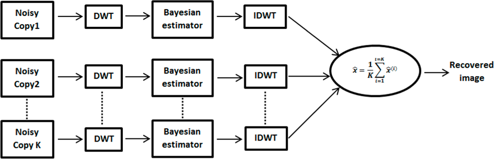
2.1. Bayesian Denoising Algorithm in the Wavelet Domain, for Multiple Noisy Copies

Let x = {x_ij} denote the M × M matrix of the original image to be recovered. The signal x is transmitted over a Gaussian additive noise channel K times, and there are K copies of noisy TEM observation at the receiver:

$$y^{(k)}=x+{\epsilon }^{(k)},k=1,\dots ,K$$

(1)

For the k-th copy, $\{{\epsilon }_{ij}^{(k)}\}$ are iid Gaussian $N(0,{({\sigma }_{ϵ}^2)}^{(k)})$, where ${({\sigma }_{ϵ}^2)}^{(k)}$ is the noise variance of the k-th copy. The noise samples between different copies are assumed independent. The image is recovered in the orthogonal wavelet transform domain.

Let the discrete wavelet transform (DWT) of the noisy observation y^(k) = x + ε^(k) be denoted by:

$$D(y^{(k)})=D(x)+D({\epsilon }^{(k)})=D(x)+{\zeta }^{(k)}$$

(2)

The wavelet coefficients (or more precisely the coefficients of the DWT) are often grouped into subbands [9] of different scales and orientations, with one lowest frequency subband, and the rest are called detail subbands. Namely, the subbands HH_j, HL_j and LH_j, j = J_c,…, J − 1 correspond to the detail coefficients in the diagonal, horizontal and vertical orientations, and the subband $L{L}_{J_c}$ is the approximation or the smooth component. J_c is the coarsest scale of the decomposition. The main goal, in a denoising problem, is to estimate $\widehat{x}$ of x from y such that the expectation of the mean-squared-error (MSE) is minimized. In fact, this MSE measure which is the simple Euclidean distance between the original and denoised estimated image is also commonly proposed in the denoising community to quantitatively measure the achieved performance improvement of a denoising technique leading to the well-known SNR expressed in decibels. The optimal regularization scheme, in the minimum MSE sense, is closely related to the model of statistical prior distribution of the wavelet coefficients. Clearly, imprecise modeling of the statistical prior directly leads to deterioration in the resulting performance. It has been shown that the statistical behavior of wavelet coefficients is successfully modeled by families of heavy-tailed distributions such as the α-stable. Boubchir and Fadili [7] proposed a prior statistical model based on the α-stable densities. They used the finite mixture of Gaussians as a fast and numerically stable analytical approximation for α-stable densities in order to obtain closed-form expressions for their Bayesian denoiser. Our first contribution extends their results to the more general situation, since the Bayesian denoiser has been already successfully applied to one set of observations. Furthermore, the Bayes rules can be constructed to mimic the thresholding rules: to slightly shrink the large coefficients and heavily shrink the small coefficients. Bayes shrinkage rules result from realistic statistical models on wavelet coefficients and such models allow for incorporation of prior information about the true data [10].

More precisely, we design a structure of fusion in order to obtain the most noise-free copy possible. In this structure, the Bayesian denoiser with the scale mixture approximation to the α-stable prior is first applied to each noisy copy independently. Thus, we get a partial denoised image. The final recovered image is then obtained by computing the average of all denoised copies. This proposed structure in the wavelet domain can be viewed as a parallel distributed detection fusion (DDF) radar system with multiple sensors and a center of fusion. Each sensor, based on the noisy observation, makes an individual decision about the presence or absence of the target. The global decision is made, based on the received individual decisions according to “AND” and “OR” fusion rules. This is done for each wavelet coefficient separately. We use the approximate α-stable model [7] as a prior of the wavelet coefficients. We note, that the mean of an α-stable random variable (RV) remains an α-stable RV (see [11] for more details). Then we apply the nonparametric Bayesian denoiser to estimate the denoised wavelet coefficients. The recovered image is obtained by applying the inverse discrete wavelet transform (IDWT) of the estimated coefficients. In the following section, we explain how to extend the Bayesian denoiser to multiple corrupted copies by using a fusion structure.

2.1.1. Bayesian Denoising Algorithm for One Set of Observations

As a first step in our approaches, we consider one corrupted copy of the image (K = 1 in (1)). In our work, the applied Bayesian denoiser in the wavelet domain is based on adapting a prior statistical model for D(x) in Equation (2), and then imposes it on the wavelet coefficients to describe their distribution [7,8]. It follows from Equation (2), that for K = 1:

$$\{\begin{array}{l}{c}_{mn}=a_{mn}+{\zeta }_{mn}\hfill \\ d_{mn}^{oj}=s_{mn}^{oj}+{\zeta }_{mn}j=J_c,\dots ,J-1m,n=0,\dots ,2^j-1\hfill \end{array}$$

(3)

where c_mn is the approximation coefficient of the observed noisy image at location (m,n) and $d_{mn}^{oj}$ are the details coefficients of the observed noisy image in the wavelet domain, a_mn is the approximation coefficient of the true image x at location (m,n), $s_{mn}^{oj}$ are the details coefficients of the original image x in the wavelet domain, and j and o are the scale and the orientation respectively.

Different choices of loss function lead to different Bayesian rules and hence to different nonlinear wavelet shrinkage and wavelet thresholding rules. For example, it is well known that the L₁-loss function corresponds to the maximum a posteriori (MAP) estimator [7]. However, except for some special cases of α-stable distributions (namely α = 2), it is not easy to derive a general analytical form of the corresponding Bayesian shrinkage rule, even with the scale mixture approximation. Alternatively, the L₂-based Bayes rules are used which correspond to posterior conditional means (PCM) estimates [7,8]. The general expression (using the approximate prior probability density function PDF) of the PCM estimates of the wavelet coefficients D(x) or s (conditionally on the hyperparameters) is [7,8]:

$$\widehat{s}(d/\theta )=\frac{{\sum }_{j}p(j)\frac{d{\sigma }_j^2}{{\sigma }_j^2+{\sigma }_{ϵ}^2}\mathrm{\Phi }(d;{\sigma }_j^2+{\sigma }_{ϵ}^2)}{{\Sigma }_{j}p(j)\mathrm{\Phi }(d;{\sigma }_j^2+{\sigma }_{ϵ}^2)}$$

(4)

where θ is the hyper-parameters set θ₁ = {p(j),σ_j}, and Φ(d;θ₂) is the Gaussian noise PDF with variance ${\theta }_2={\sigma }_{ϵ}^2$.

To implement the formula in Equation (4), one has to estimate heuristically [7] θ₁ = {p(j), σ_j}, and ${\theta }_2={\sigma }_{ϵ}^2$ is estimated from the HH orientation at the finer scale using the popular robust estimator [5]:

$${\sigma }_{ϵ}=MAD(d_{mn}^{H{H}_1})\times 1.4826.$$

where MAD is the median absolute deviation. We can describe the Bayesian denoising process by the following steps:

• Step 1.
  Calculate the DWT of the noisy data as in (2) for one corrupted copy of the image.
• Step 2.
  Using (4), estimate the denoised wavelet coefficients ŝ^oj;
• Step 3.
  Reconstruct the denoised image $\widehat{x}$ by computing the IDWT from the estimated wavelet coefficients.

The complete process for the Bayesian denoiser in wavelet domain is shown in Figure 2:

2.1.2. Combining Bayesian Estimator and Averaging

The proposed structure of multiple noisy copies, based on the Bayesian denoiser in the wavelet domain, consists of four major modules: (i) a subband representation function that utilizes the wavelet transform, (ii) application of the Bayesian denoising algorithm, (iii) computation of the inverse wavelet transform from the estimated wavelet coefficients and (iv) application of the traditional averaging operation to obtain the final recovered image as shown in Figure 3. This structure can be viewed as a parallel DDF radar system with multiple sensors and a center of fusion. Each sensor, based on the noisy observation, makes an individual decision about the presence or absence of the target. The global decision is made based on the received individual decisions according to “AND” and “OR” fusion rules. For the proposed structure in this paper, our fusion rule used to obtain the final noise free image is the averaging operation.

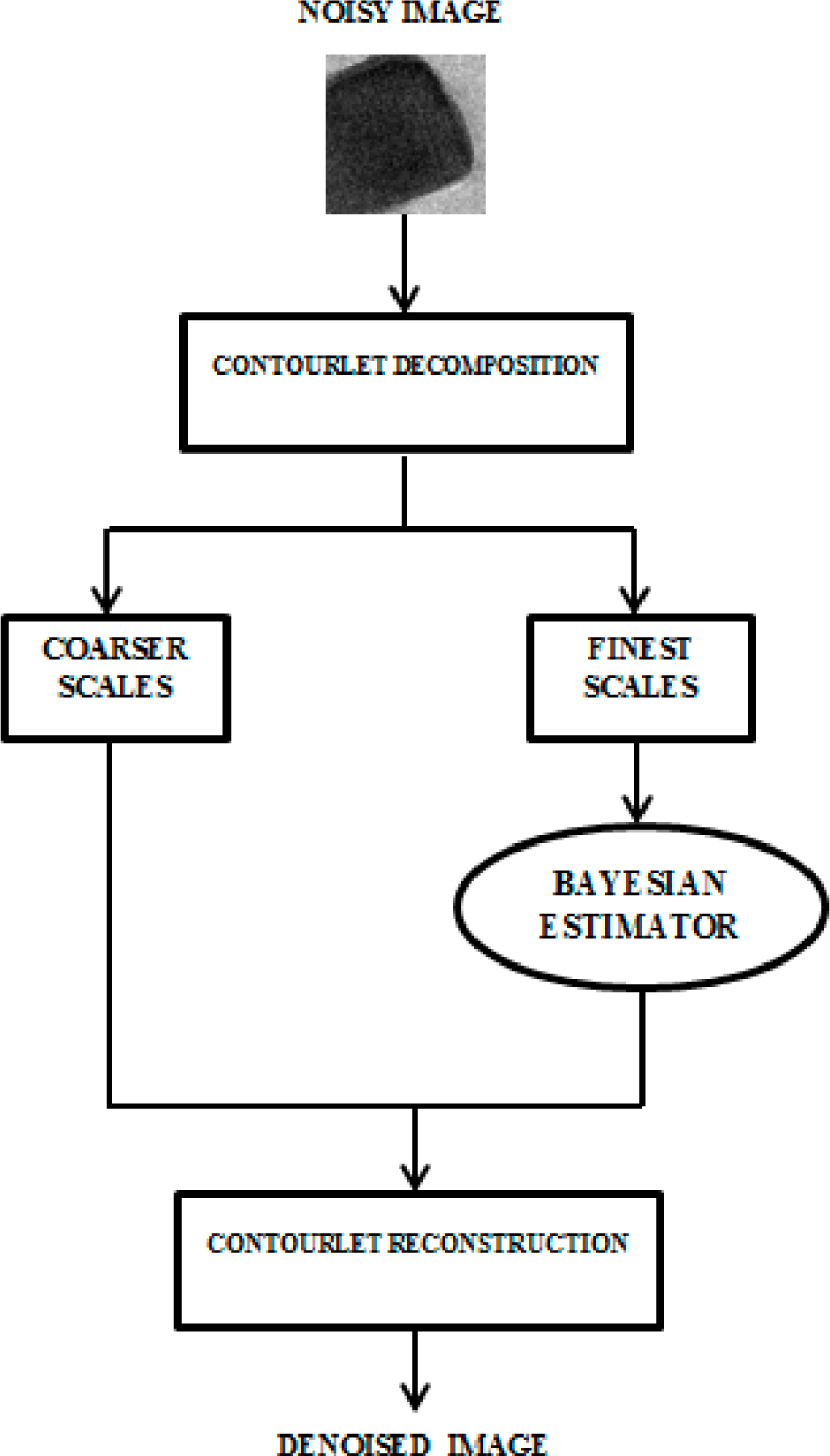
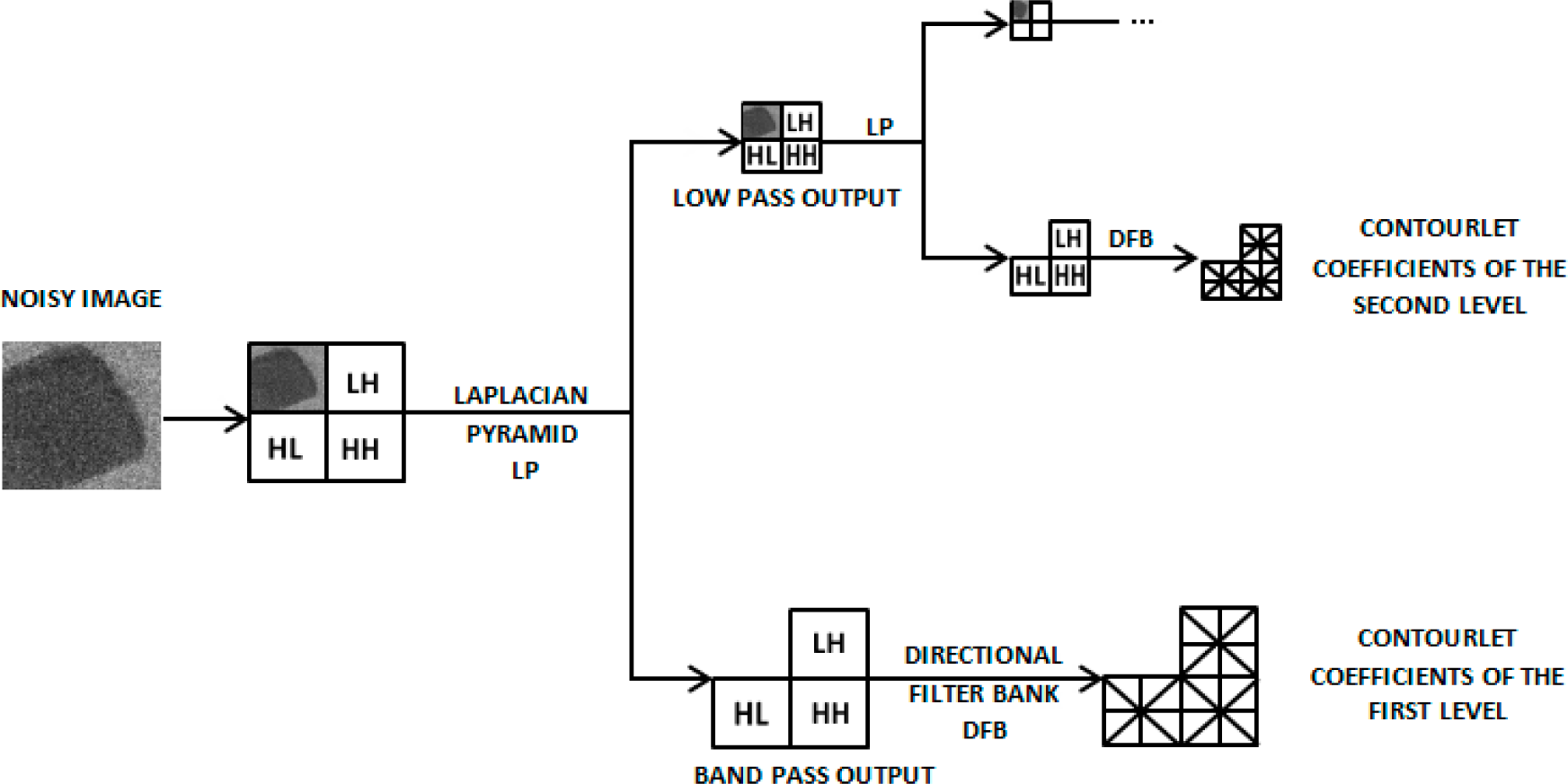
2.2. Bayesian Denoising Algorithm in the Contourlet Domain

The contourlet transform (CT), as a directional multiresolution image representation is an extension of the wavelet transform that is used to handle the inability of the DWT to accurately capture the image edges [6]. Its efficient filter bank construction, as well as low redundancy makes it an attractive computational framework for various image processing applications [9]. In this paper, we propose a new denoising method that merges of the CT and the nonparametric Bayesian estimation as shown in Figure 4.

The Laplacian pyramid at each level generates a low pass output (LL) and a band pass output (LH, HL, and HH). The band pass output is then passed into Directional Filter Bank (DFB), which results in contourlet coefficients [12]. The low pass output is again passed through the Laplacian pyramid to obtain more coefficients and this is done until the fine details of the image are obtained. Figure 5 shows the decomposition by CT of a noisy TEM image (catalase-crystal). We notice that only contourlet that match both the location and direction of image contours produce significant coefficients. Thus, the contourlet transform effectively exploits the fact that the image edges are localized in both location and direction [12].

The contourlet transform is a linear transformation, so the contourlet coefficients of the noisy observations are also divided into two parts: the coefficients of the original image and the coefficients of the noise. Hence, the contourlet transform of the noisy observation in (1) is denoted by:

$$CT(y^{(k)})=CT(x)+CT({\epsilon }^{(k)})=CT(x)+{\zeta }^k$$

(5)

For one set of observations, (k = 1 according to (2)), the output after the Laplacian pyramid (LP) stage is J bandpass noisy images, j = 1, 2, … , J in the fine-to-coarse order and a lowpass noisy image.

The specific procedure for our second proposed denoising method based on the previously developed Bayesian denoiser in the CT domain, is as follows:

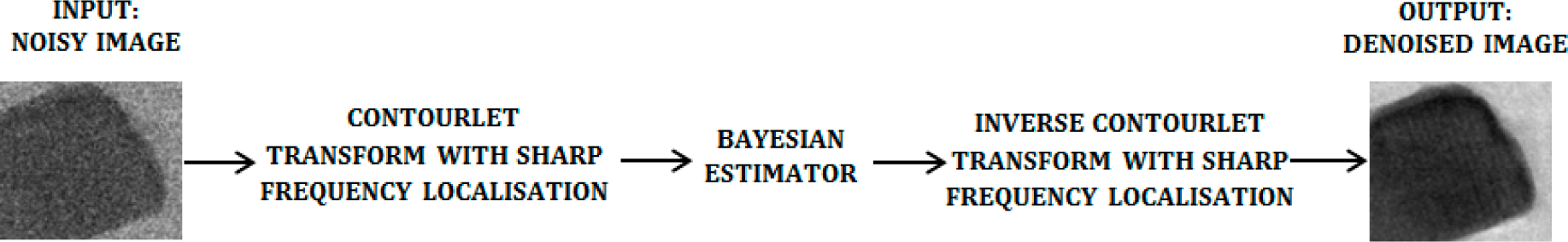
• Perform multiscale decomposition of the noisy image in the CT domain, obtain the subbands coefficients of the noisy image in different directions and levels;
• Estimate the denoised coefficients of bandpass subbands based on the Bayesian denoiser using Equation (3);
• After the denoising procedure, the contourlet transform is calculated from the processed subband coefficients, and the recovered image is obtained.

The complete process for the Bayesian denoiser in the CT domain is shown in Figure 3.

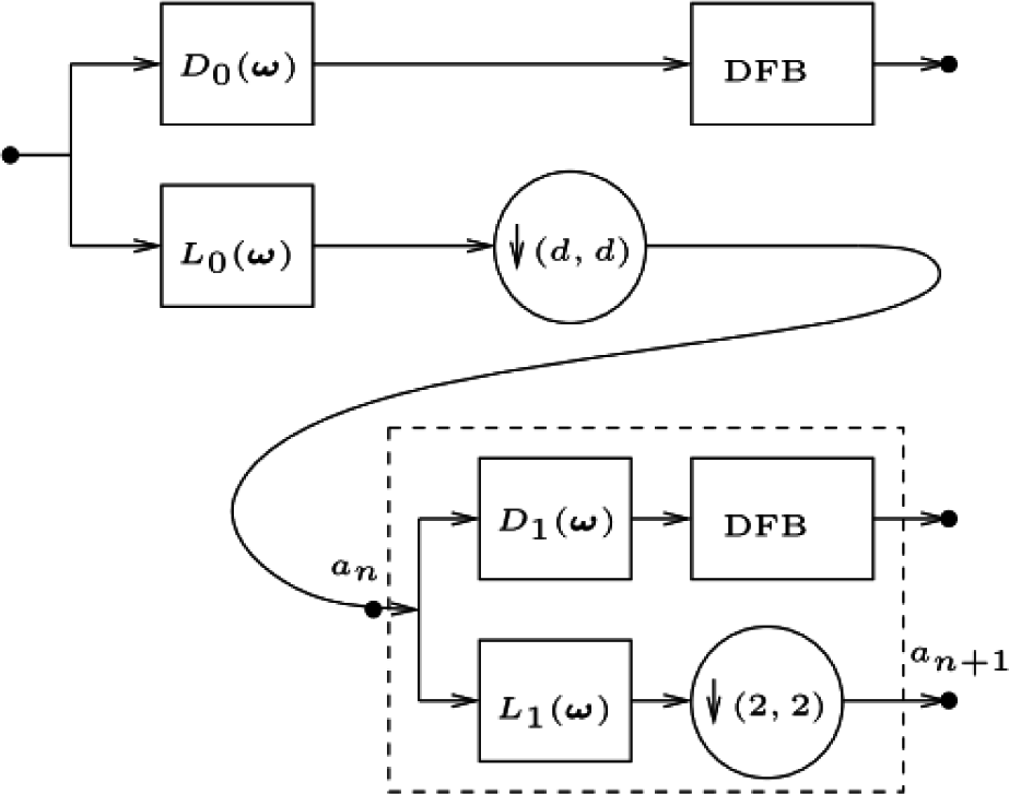
2.3. Bayesian Denoising Algorithm in the Contourlet Transform with Sharp Frequency Localization

To maximize the performance of our proposed algorithm by increasing the quality of the denoised TEM images, we propose to use the contourlet transform with sharp frequency localization (contourlet-SD) developed by Lu et al. [12]. Compared with the prior version CT, contourlet-SD greatly alleviates the non-localization problem of the contourlet and improves the regularity in the spatial domain. In this transform, Lu and Do employ a new pyramid structure for multiscale decomposition instead of the Laplacian pyramid used in the contourlet transform. The new algorithm is conceptually similar to the one used in the steerable pyramid, and it can employ different sets of lowpass and highpass filters for the first level and all other levels [12]. Figure 6 illustrates the principle the contourlet-SD.

Li(ω)(i = 0, 1), Di(ω)(i =0, 1) present lowpass filter and highpass filter respectively with $\omega \begin{array}{c}def\\ =\end{array}(\omega 1,\omega 2)$.

The lowpass filter L₀(ω) in the first level is downsampled by d along each dimension. In our experiments, we choose d = 1, so that in this case, the lowpass filter in the first level is not down sampled. The value of d is detailed in [12].

The specific procedure for our proposed denoising method, which is based on the previously developed Bayesian denoiser in the contouret-SD domain is shown in Figure 7. For the multicopy structure, we do the averaging of the outputimages for each exposure time as shown in Figure 3.

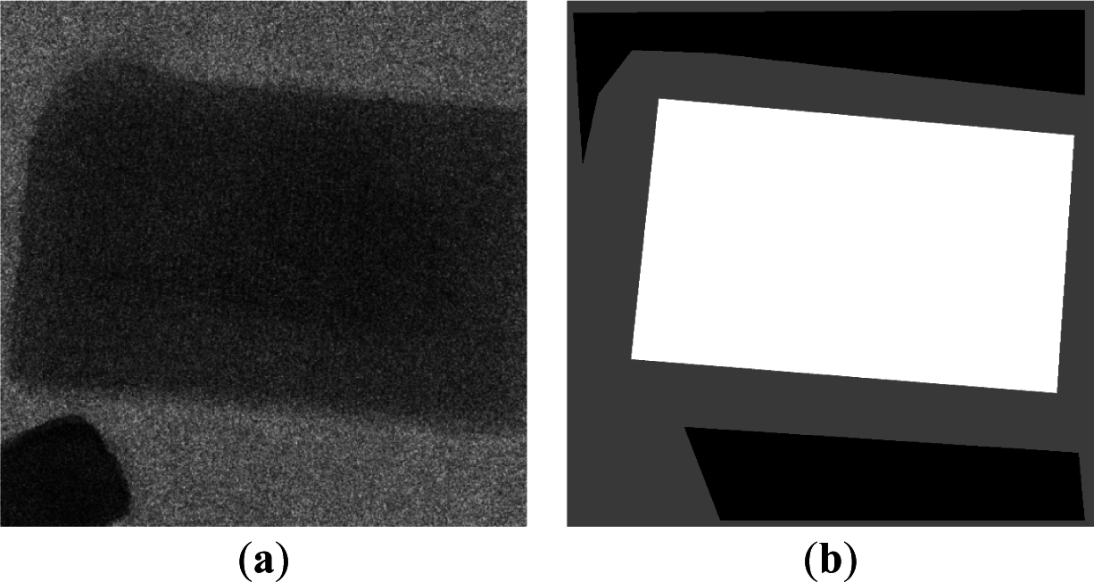
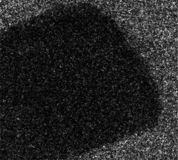
3. Test Images Dataset (Catalase)

Image filtering on electron microscopy data, which is often used to increase the contrast and the SNR of the EM images, can also significantly reduce the resolution. To evaluate these parameters (contrast, SNR, visual image quality and resolution), we used 2D catalase crystals, a well-known crystalline structure from which resolution measurements can be precisely computed using dedicated software (2dx), which is a negatively stained catalase crystals mounted on carbon-coated grids were ordered from EMS (reference 80014, EMS, Hatfield, PA, USA). Images were acquired on a JEOL 2200FS field emission gun 200 kV electron microscope (JEOL Ltd®, Tokyo, Japan) at nominal magnification of 30,000× (pixel size: 0.33 nm/px) using a GatanUltraScan 1000 (Pleasanton, CA, USA). The data acquisition occurred at different exposure times (0.05 s (20 copies), 0.1 s (10 copies), 0.2 s (five copies), 0.5 s (two copies), 1 s (one copy)), and for two zones: zone 1 and zone 2. The order of acquisitions, intentionally determined by the biologists, was taken in account as it has an effect on the images. These TEM images contain two distinct regions: noise region and object plus noise region. Transitional regions are not taken into account. We note that the original TEM images are of size 2048 × 2048. In our experiments, we have cropped these images to 512 × 512.

3.1. Denoising Quality, in the Context of Computational Performance

To accurately assess our results we calculated the SNR. However, in contrast with synthetic images where noise is added to a noiseless image (original), in the case of TEM images, the original image is not available. Thus it was necessary to define the zone where the noise is situated and the zone where our object is located. To accomplish this, we created a mask for each image using the software ImageJ 1.48 v and multiplied it by its corresponding image as shown in Figure 8. The average intensity value of the noise is calculated from the zone of noise whereas the average intensity value of the signal is calculated from the zone of our object.

Thus, the SNR is calculated using the following formula:

$${\text{SNR}}_{\mathrm{dB}}=10{\log }_{10}{\left[\frac{(Ax-A\epsilon )}{{\sigma }_{\epsilon }}\right]}^2$$

(6)

where Ax is the average intensity value of the signal, Aε is the average intensity value of the noise and σ_ε is the standard deviation of the noise.

The mask has three values (0, 1 and 2). The noise area occurs where the mask value is equal to 0. Areas where the mask value is equal to 1; are between the noise and the sample; and these areas of the image are not taken into account in the computation. A mask value is equal to 2; corresponds to areas in the image where there are both the sample and noise. This allows us to perform the calculation only at precise locations on the images. In our experiment; we zoom in close to the catalase image (512 × 512); which permits us to capture the difference between the noisy image and the denoised image; especially the contours of our catalase as shown in Figure 9.

4. Experimental Results and Discussion

In this section we present results of the one-copy structure in which each image is denoised separately, and then we show the results that were obtained using the multiple copy structure. In this latter structure, we calculated the average of the denoised images and then computed SNRout from the averaged image.

In our experiments on the Bayesian denoiser in the wavelet domain (based on our previous works [13]),we chose “sym8” as the mother wavelet and set the level decomposition equal to three to achieve the best quality in this case. For the Bayesian denoiser in the contourlet transform and the contourlet-SD, we selected the number of levels for the DFB at each pyramidal level equal to (2, 3, 4, 5) pkva filters and we did not downsample the low-pass subband at the first level of decomposition, based on [12].

4.1. For One Copy

We compare the denoising performance of the proposed Bayesian estimator in the contourlet, contourlet-SD domain and the one proposed by Boubchir [7] in the wavelet domain. First, we calculated the SNRin for all the images in zone1 before the denoising and the SNRout after we have denoised them. We have also calculated the average of SNRin and SNRout from each image series at 0.05 s, 0.1 s, 0.2 s, 0.5 s and 1 s. The values of the SNR’s are reported in

Table 1. SNRin and SNRout of the catalase 512 × 512 by applying the Bayesian estimator in the discrete wavelet transform (DWT), contourlet (CT) and the contourlet-SD (CTSD), respectively.

Images	SNRin	SNRout
		Bayesian using DWT	Bayesian using CT	Bayesian using CTSD
0.05 s_1	9.1166	13.9593	17.8131	19.6782
0.05 s_2	8.9658	13.6485	16.7772	19.2051
0.05 s_3	9.1184	14.0995	16.4769	19.0817
0.05 s_4	9.0222	13.8463	17.4416	19.1799
0.05 s_5	9.1427	14.2458	16.5566	18.6347
0.05 s_6	9.0856	13.9043	17.5439	19.9940
0.05 s_7	8.9427	13.7417	17.5398	20.3357
0.05 s_8	8.7014	13.7578	17.4200	18.1818
0.05 s_9	8.8151	13.8131	16.2238	18.5918
0.05 s_10	9.2293	14.5171	16.6850	19.6981
0.05 s_11	8.9786	14.0618	17.8385	19.9707
0.05 s_12	8.8766	13.6726	18.1250	19.2492
0.05 s_13	8.7797	13.7597	16.4788	18.4656
0.05 s_14	9.2302	13.9938	18.1627	19.0698
0.05 s_15	8.7073	13.9168	17.2837	18.4448
0.05 s_16	8.9424	13.9458	16.9121	21.3077
0.05 s_17	8.6589	13.4699	17.4719	18.5097
0.05 s_18	9.2351	14.3087	16.4817	19.8011
0.05 s_19	8.7326	13.4320	16.5471	18.0423
0.05 s_20	8.9453	13.9619	15.8638	19.5211
Average_0.05 s	8.961325	13.90282	17.08216	19.24815
0.1 s_1	15.7499	20.0007	22.3827	23.7175
0.1 s_2	15.5526	19.9711	21.8719	23.9655
0.1 s_3	15.9268	20.5442	22.3254	24.4462
0.1 s_4	15.6543	19.6158	24.3029	24.7552
0.1 s_5	15.4476	19.4643	22.4469	23.7101
0.1 s_6	16.2155	20.4828	24.2061	24.9250
0.1 s_7	14.3256	18.3053	20.7924	22.0617
0.1 s_8	14.0977	18.2095	20.6396	21.8724
0.1 s_9	13.0810	16.6382	18.3037	20.4235
0.1 s_10	15.2419	19.3726	22.8133	24.7107
Average_0.1 s	15.12929	19.26045	22.00849	23.45878
0.2 s_1	22.9465	26.8124	29.2039	30.6730
0.2 s_2	22.7931	26.6525	28.9076	30.4631
0.2 s_3	22.6746	26.3368	29.0428	30.7096
0.2 s_4	22.8597	26.7064	29.4987	30.5284
0.2 s_5	22.9655	26.9566	29.6484	30.5413
Average_0.2 s	22.84788	26.69294	29.26028	30.58308
0.5 s_1	28.9003	31.4976	33.1765	33.7052
0.5 s_2	28.9398	31.6083	33.5279	33.9979
Average_0.5 s	28.92005	31.55295	33.3522	33.85155
1 s	33.1927	35.2226	36.0073	36.6940

.

Figure 10 shows the catalase image before and after denoising using the proposed methods. These images enable us to evaluate the catalase quality after they are denoised.

From Table 1, we can see that we have significantly improved SNRout for all tested images in the contourlet transform compared with the one proposed by Boubchir [7] in the wavelet transform. Figure 9 shows the comparative results between the Bayesian denoiser-based method and the proposed algorithm using the contourlet transform. From these visual quality results, we infer that the new proposed algorithm using the contourlet transform outperforms the Bayesian denoiser-based method in the wavelet transform domain. However, unfortunately we did not neglect some of the fuzzy artifacts which appeared in the denoised images. These artifacts (mentioned in [6]) contribute to one of the major drawbacks in adopting this method. For this reason, we have proposed the contourlet-SD instead of the contourlet, in order to ensure noise reduction as well as alleviate the artifacts. As expected, Table 1 shows that SNRout-after we denoised the catalase using the Bayesian denoiser in the contourlet-SD is higher than the one applied in the wavelet transform domain and the one applied in the contourlet transform domain. Also, we can see from Figure 9d that the contourlet-SD has the capacity to result in a better images quality. Our methods clearly improve the performance of the Bayesian denoiser in the wavelet transform, but this is not enough in terms of the obtained quality; thus, we proposed the structure of multiple noisy copies.

4.2. For Multiple Noisy Copies

For the multiple noisy copies, we compared the denoising performance of the proposed methods by calculating SNRout for different number of copies. SNRin is the averaged SNRin of each series in Table 1.

Table 2. SNRout results of the proposed denoising methods using the multiple noisy copies structure.

Images	The average of SNRin	Number of copies	SNRout
			Bayesian using DWT	Bayesian using CT	Bayesian using CTSD
0.05 s	8.961325	3	22.4353	25.6364	27.3479
		5	26.4296	29.3206	30.8367
		7	28.7677	31.5373	32.9777
		9	30.4237	33.0430	34.2913
		11	31.7434	34.1565	35.3560
		15	33.3985	35.5766	36.5513
		17	33.8908	35.9850	36.9173
		20	34.7928	36.7953	37.6634
0.1 s	15.12929	3	28.0105	29.7354	30.9450
		5	31.5391	33.1076	33.9182
		7	33.8048	35.1647	35.8558
		10	34.7072	35.5889	36.1114
0.2 s	22.84788	2	31.1815	33.2577	34.5045
		3	33.7801	35.6552	38.1932
		5	36.7699	38.5647	39.1394
0.5 s	28.92005	2	34.4354	35.8070	36.1945

shows the obtained results.

Figure 11a,b show the 0.05 s_1 catalase image before and after denoising using seven and twenty copies respectively. Knowing that, these images are very noisy as they use a very low exposure time during their acquisition.

From Table 2, it can be seen that our methods achieve the best results-in term of SNR values and visual quality in all situations. We achieve these results in both contourlet and contourlet-SD implementations. These enhancements can be easily seen especially for low exposure time images (0.05 s). By combining twenty 0.05-second copies, the achieved SNRout is a higher than the SNRout of the catalase image at 1 s. Figure 11 shows the catalase 0.05 s before and after denoising using the multiple noisy copies structure. The proposed methods gave better visual quality with the noise mostly removed in the smooth regions and also along the edges. We attribute the superior performance of our algorithm to the directional multiresolution image representation of the contourlet, as it can efficiently capture and represent singularities along smooth object boundaries in natural images. Basing our proposed denoising algorithms on the contourlet transform, the estimation of the processed coefficients is not only done in a limited number of directions as in the DWT representation, but in multiple resolutions and multiple directions. These interesting results are exactly what we have been looking for. The algorithms solve the problem of the low SNR resulting from the very low electron doses used during the acquisition of the biological specimen in order to avoid damages to the specimen. In Figure 12, we compare the multi-copies structure results after denoising the catalase 0.05 s (very low exposure time) and the catalase 1 s (high exposure time). We clearly see that the catalase at 0.05 s after denoising outperforms the catalase at 1 s not only in term of the value of the SNR but also in term of the visual quality.

5. Concluding Remarks

This paper investigates methods for denoising TEM images that are acquired with a very low exposure time. We proposed to merge the Bayesian estimator in the contourlet which offers directionality and anisotropy to image representation that are not supported by the wavelet transform [14]. We also proposed to combine the Bayesain estimator and the contourlet transform with much better localization in the frequency domain and regularity in the spatial domain [12]. We studied the proposed denoisers under two main cases: one copy and multiple copy noisy images. For the one copy structure we denoised each image separately then calculated its SNRout. For the multiple copy structure we calculated the average of the denoised images (pictured with the same exposure time) then computed its SNRout. Experimental results on real TEM data show that the proposed methods succeeded in improving the Bayesian estimator by giving higher SNR and better quality which lead us to suggest the acquisition of multi-copies of the biological specimen at a very low exposure time instead of a one copy in a high exposure time. Then, we apply our multi-copy denoising structures using the Bayesian denoiser in the contourlet domain and the contourlet-SD. This gives better results and avoids the problem of biological sample sensitivity. It also improves the accuracy of the alignment step during 3D tomographic reconstruction.

References

1. Zuo, J.M. Electron detection characteristics of a slow-scan CCD camera, imaging plates and film, and electron image restoration. Microsc. Res. Tech 2000, 49, 245–268. [Google Scholar]
2. Henderson, R. Realizing the potential of electron cryo-microscopy. Q. Rev. Biophys 2004, 37, 3–13. [Google Scholar]
3. Miloš, V.; Raimond, B.G.; Lucas, J.V.; Abraham, J.K.; Ivan, L.; Uwe, L.; Hans, R.; Ozan, Ö.; Bernd, R. Image formation modeling in cryo-electron microscopy. J. Struct. Biol 2013, 183, 19–32. [Google Scholar]
4. Donoho, D.L; Johnstone, I.M. Ideal spatial adaptation by wavelet shrinkage. Biometrik 1994, 81, 425–455. [Google Scholar]
5. Donoho, D.L. De-noising by soft-thresholding. IEEE Trans. Inf. Theory 1995, 41, 613–627. [Google Scholar]
6. Do, M.N.; Vetterli, M. The Contourlet Transform: An efficient directional multiresolution image representation. IEEE Trans. Image Process 2005, 14, 2091–2106. [Google Scholar]
7. Boubchir, L.; Fadili, J.M.A. Closed-form nonparametric Bayesian estimator in the wavelet domain of images using an approximate α-stable prior. Pattern Recognit. Lett 2006, 27, 1370–1382. [Google Scholar]
8. Boudjelal, A.; Messali, Z.; Boubchir, L.; Chetih, N. Nonparametric Bayesian estimation structures in the wavelet domain of multiple noisy image copies. Proceedings of the 6th International Conference on Sciences of Electronic, Technologies of Information and Telecommunications, Sousse, Tunisia, 21–24 March 2012; pp. 495–501.
9. Ouahabi, A. Signal and Image Multiresolution Analysis; Wiley-ISTE: Hoboken, NJ, USA, 2012. [Google Scholar]
10. Fabrizio, R.; Brani, V. Bayesian Modeling in the Wavelet Domain; Handbook of Statistics 25 Bayesian Thinking—Modeling and Computation; Elsevier: Amsterdam, The Netherlands, 2005; pp. 315–338. [Google Scholar]
11. Nikias, C.L.; Shao, M. Signal Processing with Alpha-Stable Distributions and Applications, 1st ed; Adaptive and Learning Systems for Signal Processing, Communications and Control Series; Wiley: New York, NY, USA, 1995. [Google Scholar]
12. Lu, Y.; Do, M.N. A new contourlet transform with sharp frequency localization, Proceedings of the 2006 IEEE International Conference on Image Processing, Atlanta, GA, USA, 8–11 October 2006; pp. 1629–1632.
13. Sid Ahmed, S.; Messali, Z.; Ouahabi, A.; Trépout, S.; Messaoudi, C.; Marco, S. Bilateral filtering and wavelet based image denoising: Application to electron microscopy images with low electron dose. Int. J. Netw. Secur 2013, 1, 1–12. [Google Scholar]
14. Angshul, M.; Arusharka, B. A comparative study in wavelets, curvelets and contourlets as feature sets for pattern recognition. Int. Arab J. Inf. Technol 2009, 6, 47–51. [Google Scholar]
Figure 1. Basic principle of Transmission Electron Microscopy (TEM).
Entropy 17 03461f1
Figure 2. Flowchart of the Bayesian denoiser.
Entropy 17 03461f2
Figure 3. Denoising of multiple noisy copies based on the Bayesian estimator and averaging.
Entropy 17 03461f3
Figure 4. Structure of the Bayesian estimator in the contourlet transforms
Entropy 17 03461f4
Figure 5. Illustration of contourlet transform.
Entropy 17 03461f5
Figure 6. Block diagram of the contourlet transform with sharp frequency localization. Only the analysis part is shown, as the synthesis part is exactly symmetric.
Entropy 17 03461f6
Figure 7. Illustration of the denoising method based on the contourlet transform with sharp frequency localization.
Entropy 17 03461f7
Figure 8. (a) The catalase image 2048 × 2048, zone 1, and exposure time 0.1 s. (b) Mask of the catalase image 2048 × 2048, zone 1, and exposure time 0.1 s.
Entropy 17 03461f8
Figure 9. Enlargement of the catalase image 512 × 512, zone 1, and exposure time 0.05 s.
Entropy 17 03461f9
Figure 10. (a) The original image 0.1 s_1. (b) The Bayesian estimator in the DWT. (c) The Bayesian estimator in the contourlet transform. (d) The Bayesian estimator in the contourlet-SD. (e) The zoom of the original image 0.1 s_1. (f) The zoom of the image 0.1 s_1 denoised by using the Bayesian estimator in the DWT. (g) The zoom of the image 0.1 s_1 denoised by using the Bayesian estimator in the contourlet transform. (h) The zoom of the image 0.1 s_1 denoised by using the Bayesian estimator in the contourlet-SD.
Entropy 17 03461f10
Figure 11. (a) Original image 0.05 s_1 before denoising. (b) The averaged catalase (seven copies) using the Bayesian estimator in the DWT. (c) The averaged catalase (seven copies) using the Bayesian estimator in the CT. (d) The averaged catalase (seven copies) using the Bayesian estimator in the contourlet-SD. (e) The averaged catalase (20 copies) using The Bayesian estimator in the DWT. (f) The averaged catalase (20 copies) using the Bayesian estimator in the CT. (g) The averaged catalase (20 copies) using the Bayesian estimator in the contourlet-SD.
Entropy 17 03461f11
Figure 12. (a) Original image 0.05 s_1 before denoising. (b) The averaged catalase (20 copies) using the Bayesian estimator in the contourlet-SD. (c) Original image 1 s before denoising. (d) The denoised image 1 s using the Bayesian denoiser in the contourlet-SD transforms.
Entropy 17 03461f12