Article

Kinetic Theory Modeling and Efficient Numerical Simulation of Gene Regulatory Networks Based on Qualitative Descriptions

1
GeM , Ecole Centrale de Nantes, 1 rue de la Noe, 44300 Nantes, France
2
IRCCyN, Ecole Centrale de Nantes, 1 rue de la Noe, 44300 Nantes, France
3
LAMPA, ENSAM Angers, 2 Boulevard du Ronceray, BP 93525, 49035 Angers Cedex 01, France
4
Universidad de Zaragoza. Maria de Luna, s.n., E-50018 Zaragoza, Spain
*
Author to whom correspondence should be addressed.
Entropy 2015, 17(4), 1896-1915; https://doi.org/10.3390/e17041896
Submission received: 31 December 2014 / Revised: 25 March 2015 / Accepted: 30 March 2015 / Published: 1 April 2015

Abstract

:
In this work, we begin by considering the qualitative modeling of biological regulatory systems using process hitting, from which we define its probabilistic counterpart by considering the chemical master equation within a kinetic theory framework. The last equation is efficiently solved by considering a separated representation within the proper generalized decomposition framework that allows circumventing the so-called curse of dimensionality. Finally, model parameters can be added as extra-coordinates in order to obtain a parametric solution of the model.

1. Introduction

Using mathematical modeling to address large-scale problems in the world of biological regulatory networks has become increasingly necessary given the quantity of data made available by improved technology. In the most general sense, modeling approaches can be thought of as being either quantitative or qualitative. Quantitative methods, such as ordinary differential equations or the chemical master equation, are widespread in the literature [111]; when the model is well developed, the detail therein can be incredibly informative. However, these methods are not well suited for all applications. Quantitative models require in-depth knowledge of the reaction kinetics and generally fail as the problem size grows. The alternative approach, qualitative models, does not possess the same amount of detail, but captures the essential dynamics of the system. In addition, qualitative models have a variety of analysis tools that can be applied regardless of the problem size. Gene regulation, as a sub-genre of biological regulatory networks, is characterized by large numbers of interconnected species whose influences depend on passing some threshold, thus largely sigmoidal behaviors. The application of qualitative methods to these systems can be highly advantageous to the modeler.
In this work, we begin by considering the qualitative framework of process hitting, revisited briefly in Section 2.1. A highly flexible model, process hitting captures the most important dynamics of the system with a relatively simple syntax. The structure of this syntax lends itself to powerful static analysis tools, which can be used to answer some of the most important questions about the model, such as steady states or reachability, without constructing the state space. Realistic models in gene regulation are immense and highly interconnected: even when considering a Boolean space, the very enumeration of the possible states of the resulting system creates a combinatorial explosion. This is a frequent obstacle in the field of computer science and has been dubbed the curse of dimensionality. However, there are some questions for which one must access the underlying probability distribution associated with the Markov transitions of the qualitative model as described in Section 2.2. In addition, gaining access to the probability distribution allows for a qualitative and intuitive analysis of the system as a whole. The most pervasive methods have historically been simulation-based, although there are some instances in which this becomes computationally infeasible. Here, we propose a method to solve the system by treating the Markov equations of a process hitting model with numerical techniques. A reduced-basis method, the proper generalized decomposition (PGD), can be used to overcome the curse of dimensionality and provide fast, computationally inexpensive solutions to an otherwise intractable problem, as discussed in Section 2.3. The fact of using numerical approaches usually employed in quantitative analysis to perform qualitative analysis (addressed in general by using discrete techniques, like process hitting) constitutes the main originality and novelty of the present work. The proposed approach allows calculating a sort of qualitative probability distribution that cannot be easily obtained by using standard discrete strategies. In addition, PGD has certain qualities particularly favorable for applications to gene regulatory networks. Unknown parameters can easily be incorporated into the model at the cost of another dimension, as demonstrated in Section 3.

2. Methodologies

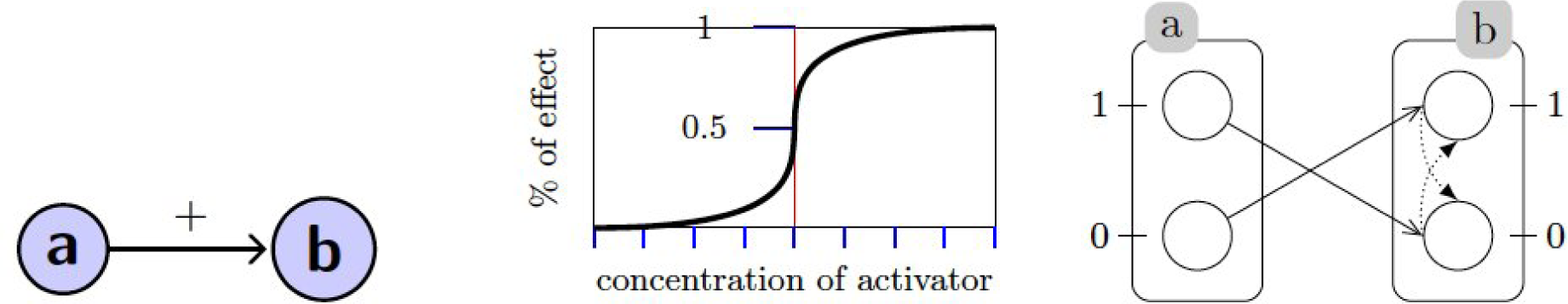
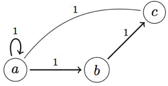
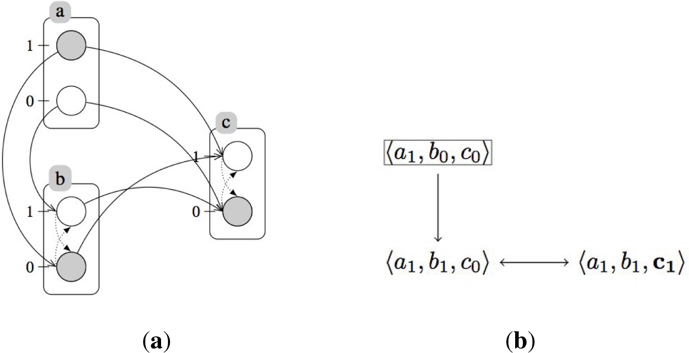
2.1. Qualitative Modeling: Process Hitting

Process hitting is a powerful, simple tool for the analysis of large regulatory networks. Historically related to the discrete models of Stuart Kauffman [12] and René Thomas [13], process hitting attempts to address problems of scalability in classical modeling methods, while maintaining the highest degree of expressiveness possible. Formally a subclass of asynchronous automata, it relies on large degrees of abstraction to describe the system as a whole. All interacting species, whether they be enzymes, genes or proteins, are abstracted as sorts. These sorts are then subdivided into processes, which could represent concentration levels, spatial configuration or any other form that has a distinct qualitative impact on the system.
Processes interact with one another via actions, in which processes hit one another to create a bounce to some new level of the same sort at a given rate. For gene regulatory networks, processes are often abstractions of relevant concentration ranges, discretized domains of real numbers and actions representing activation and inhibition reactions. Figure 1 illustrates how to define sorts, processes and actions from a biological understanding of an interaction. Process hitting relies on the initial construction of the most permissive dynamics, otherwise called generalized dynamics, in which no restrictions are placed on the potential behaviors. An example of this can be seen in Figure 1.
The general dynamics may then be successively enriched by the addition of cooperative sorts in order to best capture some known biological behaviors or eliminate undesirable behaviors. Cooperative sorts represent not species, but rather, the combined effects when multiple regulators interact cooperatively on a single target. These sorts are the combined space of the original species; thus, they must be updated, such that the current state of the cooperative sort is compatible with the current state of each of its components. A visual explanation of the construction of a cooperative sort and its refinement of a process hitting model can be found in Figure 2.
Although this is a very simplistic representation of the inner kinetics of a biological process, process hitting semantics allow us to easily model interactions with only partial knowledge of the logical functions encoded therein and pave the way for powerful static analysis techniques in order to study fixed points, reachability and cut sets, which determine the minimum criteria for reachability, in spite of the present combinatorial explosion [15,16]. Examples of process hitting at work can be found in Section 3, where we use static analysis to compare the fitness of the generalized dynamics model with that of the refined model. Furthermore, these tools are freely available online in a software called PINT. We will not attempt to expound completely on the details of process hitting here, but rather, point those interested towards [16] for a formal and thorough introduction to the modeling framework. As we progress to a biological application in Section 3, greater clarity will be given to the concepts described above, including the relevance of cooperative sorts and the power of static analysis. For a more detailed overview of process hitting (PH), the reader can refer to Appendix A.

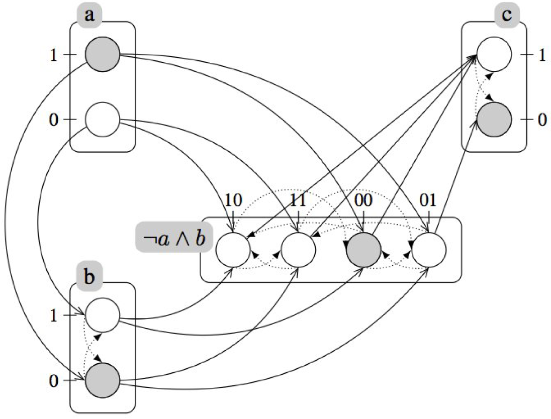
2.2. Treating Qualitative Systems with Numerical Techniques

In order to address process hitting’s global results, that is the full and complete description of the systems behavior given an initial condition, we must consider the framework in a stochastic context. Process hitting actions move the system from one state to another.
We consider n different chemical species (sorts, including cooperative sorts) S i, i = 1,…, n, each one having Ki + 1 possible levels (processes) si ∈ (0, 1, …, Ki), i = 1, …, n, and a set of m reactions (hits) Rj, j = 1, …, m, with propensity aj encoding the reaction rate:
χ j , 1 s 1 S 1 + + χ j , n s n S n a j χ j , 1 + s 1 + S 1 + + χ j , n + s n + S n
with χj,i controlling the appearance of sort Si in reaction j. For that purpose, χ is a Boolean variable, i.e., χj,i = (0, 1).
The system state is defined from z = (s1, …, sn). Thus, reaction j transforms the state z ^ = ( s 1 , , s n ) into z, with z = z ^ + v j, v j = ( s 1 + s 1 , , s n + s n ).
As a memoryless random walk, each action corresponds to a Markov equation, the so-called chemical master equation (CME), which tracks the net change in the probability of existing at a certain state and time Ψ(z, t):
d Ψ ( z , t ) d t = j = 1 m a j ( z v j , t ) Ψ ( z v j , t ) a j ( z , t ) Ψ ( z , t )
with the propensity aj depending on the system state and time.
The result is a system of linear, time-dependent, differential equations, defined given an initial condition. Some of the most famous and broadly-used techniques for addressing problems such as these have been simulation based. Simulation can become computationally expensive with respect to computing time and available memory when addressing highly multidimensional models, as in the case of Equation (2), when the number of species increases. An alternative approach is the direct application of a numerical method to the Markov equations. Here, we propose proper generalized decomposition (PGD) as an effective and well-suited technique for gene regulatory networks.
PGD [10,1720] is a multi-linear numerical solver that assumes that the target, in this case the probability distribution Ψ(z, t), can be written as a sum of a product of separable functions of the interacting species, Fi(si), i = 1, … n, and time, Ft(t):
Ψ ( z , t ) = Ψ ( s 1 , , s n , t ) k = 1 Q ψ k ( z ) F t k ( t ) = k = 1 Q F 1 k ( s 1 ) F 2 k ( s 2 ) F n k ( s n ) F t k ( t )
In essence, PGD is very close to tensor approximation-based strategies that were successfully considered for solving the CME in [21].
PGD is performed iteratively, starting at some arbitrary guess and searching for sets of functions, one functional product at a time, which will minimize the residual of the running sum. These functions are colloquially called modes; however, since the only objective is the reduction of the residual, there is no underlying notion that they represent the greatest source of variance, as is the case with principal component analysis. Although the accuracy increases with the number of modes considered in the finite sum decomposition, we assume that only a limited numberQof functional products are needed to capture the behavior of the system.
The calculation of functions involved in the separated representation is performed on the fly, from the weak form related to the CME (2):
Ω × Ψ ( z , t ) d Ψ ( z , t ) d t d z d t = Ω × Ψ ( z , t ) { j = 1 m a j ( z v j , t ) Ψ ( z υ j , t ) a j ( z , t ) Ψ ( z , t ) } d z d t
where z ∈ Ω = ω1 × … × ωn, ωi = (0, 1, …, Ki) and t I = ( 0 , T ]. In fact, the domains ωi in which the species levels are defined being discrete, the integral in ωi reduces to a discrete sum.
As just indicated, the algorithm proceeds iteratively, by computing one term of the finite sum at each iteration. If we assume that at iteration p − 1 the solution writes:
Ψ p 1 ( z , t ) = k = 1 p 1 ψ k ( z ) F t k ( t ) = k = 1 p 1 F 1 k ( s 1 ) F 2 k ( s 2 ) F n k ( s n ) F t k ( t )
at the next iteration p, the solution Ψp(z, t) reads:
Ψ p ( z , t ) = k = 1 p F 1 k ( s 1 ) F 2 k ( s 2 ) F n k ( s n ) F t k ( t ) = k = 1 p 1 F 1 k ( s 1 ) F 2 k ( s 2 ) F n k ( s n ) F t k ( t ) + F 1 p ( s 1 ) F 2 p ( s 2 ) F n p ( s n ) F t p ( t ) = k = 1 p 1 ψ k ( z ) F t k ( t ) + ψ p ( z ) F t p ( t ) = Ψ p 1 ( z , t ) + ψ p ( z ) F t p ( t )
where the unknown functions F i p ( s i ) and F t p ( t ) must be calculated.
The resulting weak form at the present iteration reads:
Ω × Ψ ( z , t ) { F 1 p ( s 1 ) F n p ( s n ) d F t p ( t ) d t } d z Ω × Ψ ( z , t ) { j = 1 m a j ( z v j , t ) ψ p ( z v j ) F t p ( t ) a j ( z , t ) ψ p ( z ) F t p ( t ) } d z d t = Ω × Ψ ( z , t ) { k = 1 p 1 F 1 k ( s 1 ) F n k ( s n ) d F t k ( t ) d t } d z d t + Ω × Ψ ( z , t ) { j = 1 m a j ( z v j , t ) k = 1 p 1 ψ k ( z v j ) F t k ( t ) a j ( z , t ) k = 1 p 1 ψ k ( z ) F t k ( t ) } d z d t
with:
ψ k ( z v j ) = F 1 k ( s 1 υ j , 1 ) F n k ( s n υ j , n ) ψ k ( z ) = F 1 k ( s 1 ) F n k ( s n ) } k = 1 , , p
The simplest test function Ψ*(z, t) within a Galerkin framework writes:
Ψ ( z , t ) = F 1 ( s 1 ) F 2 p ( s 2 ) F n p ( s n ) F t p ( t ) + F 1 p ( s 1 ) F 2 ( s 2 ) F n p ( s n ) F t p ( t ) + + F 1 p ( s 1 ) F 2 p ( s 2 ) F n ( s n ) F t p ( t ) + F t p ( s 1 ) F 2 p ( s 2 ) F n p ( s n ) F t ( t )
Introducing the test function (9) into the weak form (7) results in a nonlinear problem whose solution requires an appropriate linearization strategy. The simplest strategy consists of an alternated directions fixed point algorithm, which, considering known functions F 2 p ( s 2 ) , , F n p ( s n ), F t p ( t ) (initialized randomly), calculates F 1 p ( s 1 ). From the just updated F 1 p ( s 1 ) and F 3 p ( s 2 ) , , F n p ( s n ), F t p ( t ), function F 2 p ( s 2 ) is updated. Then, function F 3 p ( s 3 ) is updated, and so on, until calculating F t p ( t ) from the just updated F 1 p ( s 1 ) , , F n p ( s n ). Then, the iteration continues until reaching convergence, that is the fixed point that results in functions F 1 p ( s 1 ) , , F t p ( t ). Because the calculation of functions F i p ( s i ), for i = 1, ⋯, n, follows the same rationale, in Appendix B, we summarize the procedure for calculating those functions F i p ( s i ), as well as the function depending on time F t p ( t ).
Having calculated Ψp(z, t), the enrichment procedure continues for calculating using the same rationale Ψ p + 1 ( z , t ) = Ψ p ( z , t ) + F 1 p + 1 ( s 1 ) F n p + 1 ( s n ) F t p + 1 ( t ). The enrichment stops as soon as ‖ΨQ − ΨQ−1< ϵ. Alternative goal-oriented stopping criteria exist and were successfully applied in our former works [22].
For more details on the fundamental and technical details on the PGD, the reader can refer to [2326] and the references therein.
When considering a network of n species with K possible levels (for the sake of simplicity, we assume for a while that Ki = K, ∀i), solved at P time steps, the resulting complexity scales with Q · (n · K) (the complexity related to the solution of the time problem being negligible) instead of Kn involved in an hypothetical mesh or grid that should be solved P times. The separated representation is sketched in Figure 3, which emphasizes the fact that a 3D problem can be solved as a sequence of one-dimensional problems. If, for a while, we consider K = 3 and 100 terms in the finite sum decomposition, Q = 100, the complexity of the PGD solver will scale as 300n, with n the number of species involved in the network, while standard mesh-based discretizations will scale as 3n. We can notice that for n ≈ 7, both complexities become equivalent, and for n ≈ 15, the one related to the PGD is three orders of magnitude lower than the one involved in standard mesh-based discretizations.
The PGD approximation converges to the numerical solution of the problem when increasing the number of terms. To understand this fact, it suffices to realize that standard numerical solutions consist of a polynomial up to a certain degree, and a polynomial in many dimensions is no more than a finite sum of terms, each one involving the product of a function of each coordinate. This fact proves the generality of the separated representation involved in the PGD approach. The main difference with respect to standard procedures is that when considering the PGD approach, the different functions involved in these products are assumed unknown and are calculated on the fly.
It is important to note that the probability distribution obtained when applying the PGD constructor converges towards the one related to Equations (1) and (2). If these (Equations (1) and (2)) describe the true probability distribution, then the solution (3) obtained by invoking the PGD constructor will approach the true probability distribution if we consider an adequate number of terms Q in (3).
In what follows, when considering the chemical master equation formalism for qualitative modeling purposes, the possible levels of each species reduce in general to a few states, e.g., (0, 1) for expressing the presence or not of the considered species or (0, 1, 2) for indicating little, moderate or a high number of individuals in the involved species. Within the qualitative modeling framework considered in the present work, a constant rate is associated with each reaction [9]. Each reaction implies given species with given concentration levels (different concentration levels of the same species could define different reactions with their own rates). The considered rates have a significant impact in the systems dynamics. When considering the PGD framework, one can consider these rates as extra-coordinates for calculating all of the dynamics related to each choice of these rates. This possibility is specific to PGD approaches and could be used precisely for better identifying rates from experiments.
In our former works [10], we considered complex functional dependences of kinetic rates, as is usual when addressing quantitative models within the chemical master equation framework; however, and without loss of generality, in the present applications, all of the involved rates are considered constant, as is usual when considering qualitative models. Qualitative descriptions even when addressed with numerical techniques as the one here proposed can describe the main system features in a qualitative way. Analyses requiring a quantitative approach require finer descriptions and determination of the kinetic rates. Each approach (qualitative and quantitative) has its respective domains of applicability, whose comparison is out of the scope of the present work.

3. Application to a Biological Network

It is easier to understand the concepts of process hitting and PGD, as well as to see their individual and combined benefits when seen in action in the context of a realistic application towards a gene regulatory network. Here, we investigate a medium-scale model of the ErbB signaling pathway, which regulates the cell transition from the G1 to S life phase, an important checkpoint that determines whether a cell should divide, delay division or enter a quiescent state. Overexpression of ErbB is associated with many kinds of cancer, and drugs that target it and its receptor are common treatments for breast, lung and colon cancers. The directed graph for this network was taken from [27], where twenty species interact according to Boolean rules. The directed graph can be found in the Appendix for reference. We begin our application by constructing a process hitting model from this Boolean predecessor, taking the most permissive, generalized dynamics, followed by its refinement via the incorporation of cooperative sorts. The impact that this refinement has on both the statistical analysis and application of PGD will be investigated, both in terms of expressiveness and complexity. Finally, the potential of PGD’s capacity to easily incorporate model parameters as extra coordinates will be demonstrated by taking many potential values for the rates of two reactions in the directed graph.
The translation of a Boolean model to the generalized dynamics of process hitting is relatively straight forward, as shown in Figure 2: the absence of an activator effectively serves as an inhibitor and vice versa. The formal relationship between Boolean networks and process hitting can be found in [28]. At this point, we would like to investigate the model to see if it adequately reflects our biological understanding of the system as a whole: are experimentally demonstrated states reachable; are impossible states unreachable; and are there fixed points if steady-state behaviors exist? These questions constitute sanity checks, making sure our model is not essentially flawed from the beginning. The structure of the system (see Appendix C) suggests two species of experimental interest: EGF as an input, having no predecessor, and pRB as output, having no successor. Using these two species, we can easily formulate simple reachability criteria in order to perform sanity checks on our model. We consider a system at rest, in which all components begin in their inactive state. If no changes are made on the input protein, EGF when it is inactive, we expect that the system will remain at rest and that no change is to occur in the output protein. However, if EFG is introduced, the signal should be able to propagate to the output, pRB. In order to be a feasible model, the system must pass these two criteria. Results from static analysis, shown in Table 1, provide good evidence that the generalized dynamics are too permissive and do not accurately capture the biological behaviors, which are essential for a functioning model: not only are we unable to find any fixed points within the system, for which we do expect to find at least one, but the protein pRB may become sporadically activated in a globally inactive system, failing the first sanity check. Therefore, we must refine the model, incorporating the suggested logical gate rules from [27] via cooperative sorts. In doing so, we recapture these vital phenomena, finding three fixed points and passing both sanity checks. These results were obtained in a matter of seconds, using simple commands in freely available software, allowing us to efficiently alter our model before investing time in more computationally expensive analysis.

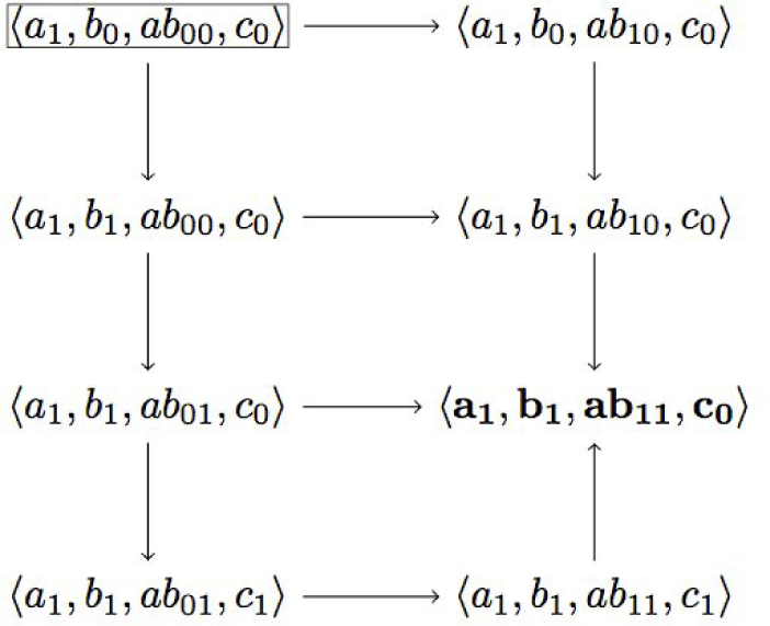
3.1. Treating Qualitative Systems with Numerical Techniques

The Markov equations of the process hitting actions provide a system of DEs to which we can apply PGD. Each species occupies a dimension of the state space. With two processes to each sort, the final problem is of size 220, or over one million possible states. The underlying probability distribution is a function of these species and time. Our goal is to approximate this solution by a summation of separable functions:
Ψ ( z , t ) k = 1 Q F E G F k ( s E G F ) F p R B k ( s p R B ) F t k ( t )
In the case of process hitting containing only the generalized dynamics, this is an appropriate and accurate method. However, once cooperative sorts are incorporated into the qualitative model, the cooperating species can no longer be represented by separable functions. To satisfy the enriched model, we may simply combine those dimensions that participate in cooperative sorts. While this does create vectors that grow exponentially with each added species, it is biologically implausible that more than three or four species would participate in a cooperative influence on a single target. Therefore, we can expect this growth to be cut short long before the dimension of a cooperative sort becomes too large. As we combine the state spaces so that they reflect their cooperative sorts, the error associated with PGD solutions as compared to the solution obtained from simulation techniques decreases.
However, what is to be done when one species participates in multiple cooperative sorts? There are two possibilities: either group species into a macro-species or leave them separated. The former possibility could blow up the state space of the combined species, due to chains of regulations forcing many species to be glued together. Hence, it may result in being unfeasible. The second one does not blow up (the state of individual species remains the same), but leads in general to more terms in the separated representation, due to the need to correct for the correlation effects of the regulation.
The solutions that we obtain from PGD are approximations of the full probability distribution corresponding to the Markov equations created by process hitting. From these probability distributions, we are able to make fast analysis of the global behaviors of the system: rather than being limited to asking the questions answerable using static analysis, a modeler can watch the system evolve through time and make general statements on the qualitative behavior.

3.2. Incorporation of Unknown Parameters

It is often the case, especially in a growing field such as genomics, that elements of a regulatory network are disputed or unknown. Researchers may come to very different conclusions about the parameters that fit a particular system. With simulation techniques, each new set of parameters requires a full repetition of all of the trials, limiting the modeler and leading to ad hoc choices made for the sake of feasibility. However, PGD offers a simple way of incorporating these unknown parameters directly into the model, making it possible to obtain an approximate solution for a range of values all at once [10,29]. The parameter is encoded as one of the separable spaces and is included at the cost of one dimension added to the overall solution space. For our example, perhaps one of the regulating reactions is difficult to study separately from the system as a whole, say interactions involving p27 and p21. Unlike the first half of the directed graph, which is simply an activation cascade, these proteins are involved in both inhibiting and activating relationships, so changes to their rate laws should more greatly influence the final expression of pRB. We would like to incorporate many potential values of the action firing rate r into our model, anywhere between two times faster 2r and two times slower 2/r than the other reactions in the system. Since our representation requires discretization, we consider forty equally-spaced values between r/2 and 2r. Our decomposition of Ψ(z, t) is changed slightly in order to accommodate the parameter r for the range of possible values from Ψ(z, r, t):
Ψ ( z , r , t ) k = 1 Q F E G F k ( s E G F ) F p R B k ( s p R B ) F r k ( r ) F t k ( t )
While simulation run time grows linearly with each element, 40-times longer since there are 40 values in the discretization, to obtain a result, we are able to derive a solution in relatively equal time using PGD. In Figure 4, we see three solutions for the protein pRB given different values of the rate parameter r: r/2, 3r/2 and 2r. These comparably fast results allow us to perform general analysis on the network by directly observing how the global behavior changes with parameters.

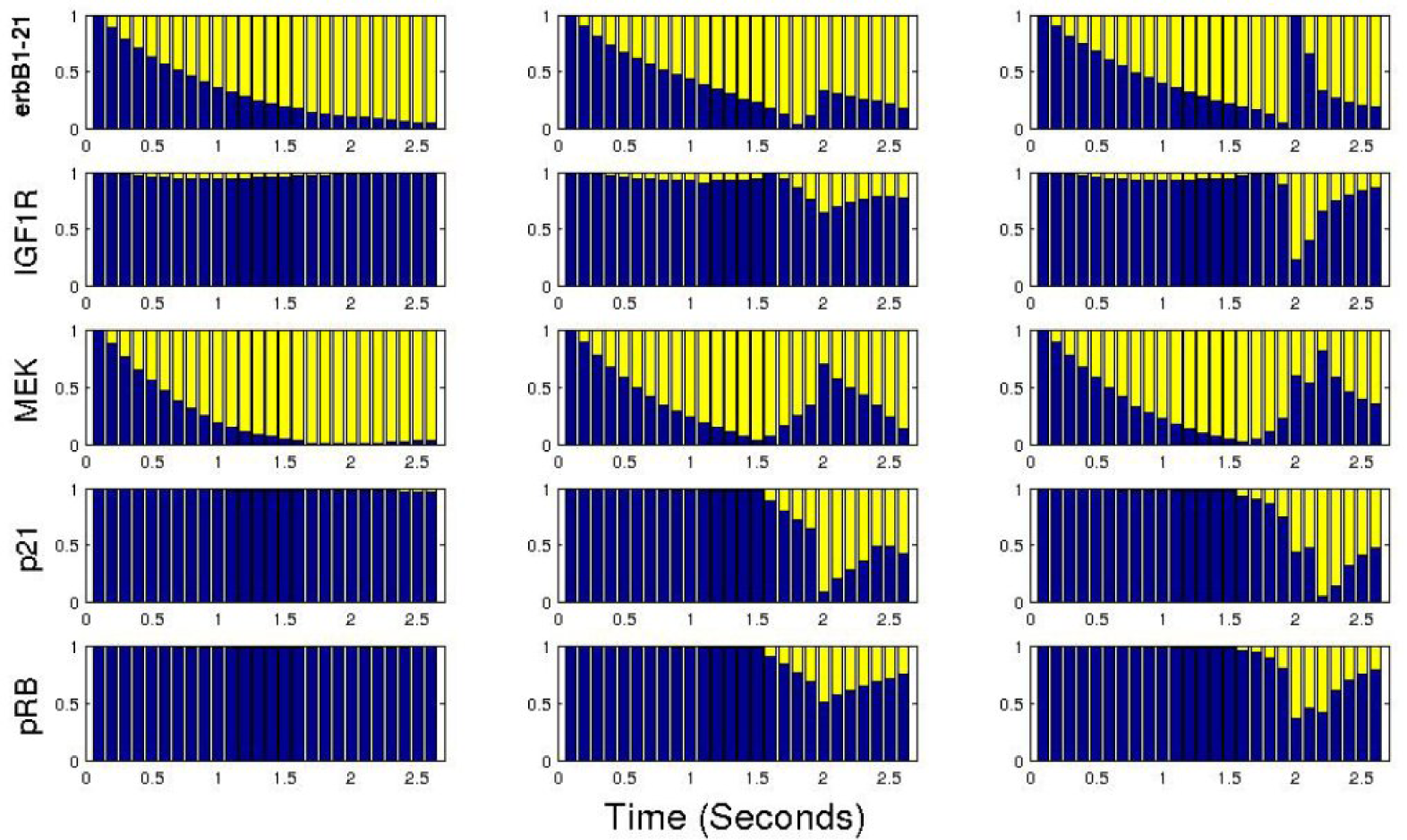
4. Evaluation and Analysis

Up to now, we have presented a new method of approaching discrete models of gene regulatory networks, uncovering briefly the origins of its individual components, process hitting and PGD, and applying it to a real biological system. As bioinformatics grows and many new methodologies are proposed, however, it is increasingly important to discuss in a straightforward manner how well our method performs, highlighting both its merits and weaknesses.
We began our approach by considering the discrete modeling framework of process hitting. This approach allows for a great extent of abstraction in the development of a regulatory model and comes with a well-developed analysis toolbox, making it an attractive starting framework. However, the application of PGD to Markov equations would be effective for any discrete modeling type that can be described as such. Process hitting does have an advantage in that the species that interact in nonlinear ways and thus must be represented together in the decomposition are well defined as cooperative sorts in the very construction of the model. Once the Markov equations have been provided, the method is relatively straightforward; PGD is a well-founded numerical method with thoroughly documented implementations.
As for the results themselves, there are several points to touch on: ease of analysis, model validation and accuracy. One of the most interesting aspects of this approach is the nature of the results: a full probability distribution as an approximate solution to a set of equations. As demonstrated in Figure 4, the output lends itself to visualization on an individual scale, that is for each protein involved. The behavior of a gene or protein can be described in very plain and qualitative terms, even for elements whose evolution is complicated and never reaches steady-state behaviors. However, the apparent behavior can only be taken at face value: while a protein may appear to oscillate or tend to a certain value, the solution is only valid for the limited time frame in which it is analyzed and is not tied to a mathematical principle governing its evolution. Furthermore, since the solution is approximative, it is possible that species whose static analysis proves total inactivation or activation would be found slightly activated or inactivated in the PGD solution, a potentially important distinction in the world of genomics. In such instances, the static analysis and numerical analysis may be found in conflict with one another, compromising the accuracy of the resulting analysis.

5. Conclusions

In the case of gene regulatory networks, there are many reasons why a modeler might choose the application of qualitative methods, one of which is process hitting. Process hitting offers many advantages for large-scale, which are often the more realistic, systems in the form of static analysis tools. These analysis tools alone, however, cannot provide the complete and intuitive solution of the system as a full probability distribution for each state over time. By translating process hitting actions to Markov equations, we are able to treat a system of PDEs directly. Proper generalized decomposition has proven efficient in solving process hitting models. As opposed to simulation techniques, which have been historically the preferred methodology, PGD can provide full solutions, including multiple unknown parameters, with a single run. Here, we have shown some of the potential of this method, applying a combination of static analysis and numerical tools in order to maximize the expressiveness and understanding of a qualitative model. Only the basic elements of process hitting have been incorporated into the Markov equations considered, that is actions with simple rate laws. Including temporal and varied stochastic features into these equations would further increase its potential.

Appendix

A. Qualitative Modeling: Process Hitting

Process hitting is a powerful simple tool for the analysis of large regulatory networks. Historically related to the discrete models of Stuart Kauffman [11] and René Thomas [12], process hitting attempts to address problems of scalability in classical modeling methods while maintaining the highest degree of expressiveness possible. Formally a subclass of asynchronous automata, it relies on large degrees of abstraction to describe the system as a whole. All interacting species, whether they be enzymes, genes or proteins, are abstracted as sorts. These sorts are then subdivided into processes, which could represent concentration levels, spatial configuration or any other form which has a distinct qualitative impact on the system.

A.1. Generalized Dynamics

Processes interact with one another via actions, in which processes hit one another to create a bounce to some new level of the same sort at a given rate. For gene regulatory networks, processes are often abstractions of relevant concentration ranges, discretized domains of real numbers, and actions represent activation and inhibition reactions. Figure 1 illustrates how to define sorts, processes and actions from a biological understanding of an interaction. Process hitting relies on the initial construction of the most permissive dynamics, otherwise called generalized dynamics, in which no restrictions are placed on the potential behaviors. An example of this can be seen in the following example.

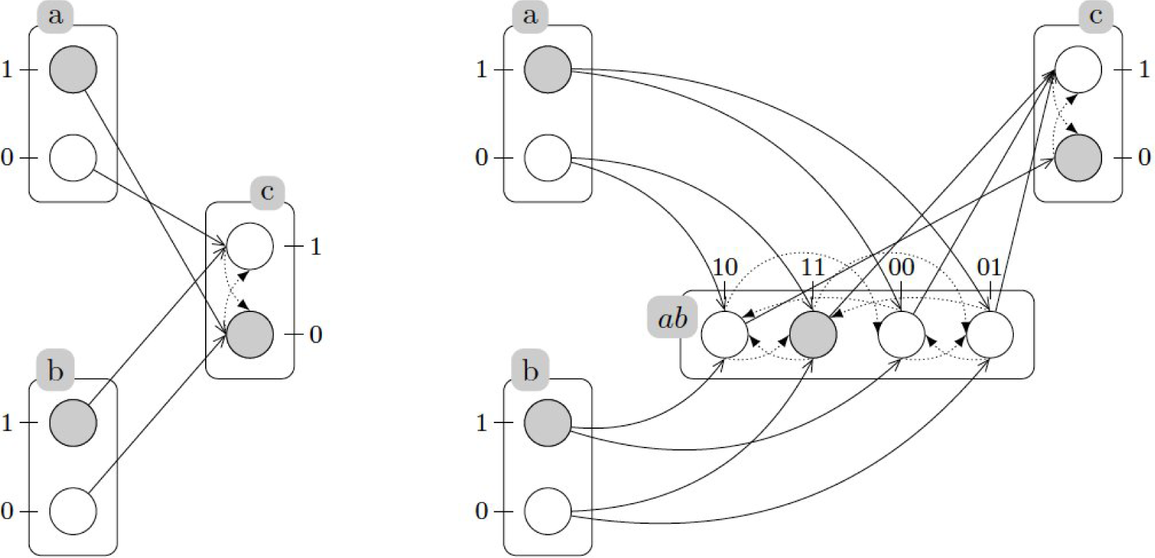
A.2. Example: Generalized Dynamics of the Incoherent Feed-Forward Loop

In order to illustrate the modeling process of a biological network using process hitting, we selected a common motif of regulatory and signaling network, the incoherent feed-forward loop [30], whose interaction graph (IG) is given in Figure 5. The network has three components: a (assumed here to be constant), which activates b, and c, which is both activated by b and inhibited by a. It is called incoherent as c is both inhibited (directly) and activated (through b) by a.
Thanks to the rules depicted above, the generalized Boolean dynamics of the IG in Figure 5 can be automatically encoded in process hitting, resulting in the actions summarized in Figure 6a.
Figure 6b draws the possible transitions from the state (a1, b0, c0) of the generalized dynamics. First b is activated by a. Then, as there is no knowledge of the cooperation between a and b and c, there cannot be any consensus on the value of c. As a result, the value of c oscillates due to the successive independent activations by b and inhibitions by a.
One can notice that the state-transition graph would have 23 states, while the process hitting model is made of 3 × 2 actions. This is an important feature of process hitting, since it makes it possible to tackle very large systems in which the number of states grows exponentially with the number of components.

A.3. Refining Dynamics with Cooperativity

The general dynamics may then be successively enriched by the addition of cooperative sorts in order to best capture some known biological behaviors or eliminate undesirable behaviors. Cooperative sorts represent not species, but rather, the combined effects when multiple regulators interact cooperatively on a single target. These sorts are the combined space of the original species; thus, they must be updated such that the current state of the cooperative sort is compatible with the current state of each of its components. A visual explanation of the construction of the refinement of a process hitting model thanks to a cooperative is given in the example below.
In process hitting, the local state change of a sort is controlled by one and only one process (the hitter). In such a setting, we may ask how to encode local state changes that should be controlled by the presence of at least two active processes. For instance, we may want that c0 bounces to c1 only if a0 and b1 are active. We call such a behavior a cooperativity between sorts a and b to act on c0. We show now how to interpret such cooperativities in process hitting.
Thus, a cooperativity can be encoded with a new sort, which will act as the logical function. Such a cooperative sort υ contains one process per state of the cooperating sorts. The intuition is that the active process of sort υ will reflect the state of all of the cooperating sorts. To do so, each cooperating process hits all processes to make it bounce to the appropriate process.
It is important to note that the proposed construction introduces a temporal shift in the application of the cooperativity. It results in potential spurious transitions when the state of the cooperative sort is incoherent with the actual state of the cooperating sorts. This behavior is somehow similar to a biological complex: the complex AB can be present, while individuals A and B are absent. In addition, such spurious behaviors can be eliminated by adding the notion of priority into process hitting to make the update of the cooperative sort happen always before any other action. However, this is out of the scope of this paper.
Overall, applied to process hitting of the generalized dynamics of an IG, the refinement using cooperativity allows the encoding of additional knowledge in the logical functions between regulators. The resulting model dynamics is smaller (in terms of possible behaviors) than the generalized one.

A.4. Example (Continued): Refined Dynamics of the Incoherent Feed-Forward Loop
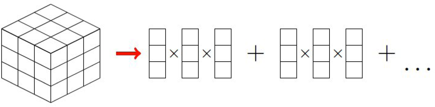
Returning to our example of the incoherent feed-forward loop, we may know that a and b cooperate for c as such: c is active if and only if a is absent and b is present. Therefore, we refine our generalized dynamics using a cooperative sort that encodes the Boolean function ¬ab, as shown in Figure 7.
In the generalized dynamics, due to the undefined cooperation between a and b when both are present, c oscillated. In our refined dynamics, this is no longer the case: c converges to c0 as a is active. Part of the transition graph is shown in Figure 8 when starting in the state (a1, b0, ab00, c0). It ends on the fixed point (a1, b1, ab11, c0). The initial process of the cooperative sort (named ab) has been intentionally chosen incoherent with the state of a and b.

B. PGD Constructor

B.1. Calculation of Functions F i p ( s i )

When assuming known, in Equation (7), functions F k l ( s k ), ∀kp; F i l ( s i ), ∀l < p, as well as F t l ( t ), ∀lp, the only unknown is F i p ( s i ). By calculating the integral in Equation (7) in ω 1 × × ω i 1 × ω i + 1 × × ω n × , it results:
ω i F i ( s i ) ( j = 1 m { γ j ( s i υ j , i ) F i p ( s i υ j , i ) γ j ( s i ) F i p ( s i ) } ) d s i = ω i F i ( s i ) g i ( s i ) d s i , F i ( s i )
which results in an algebraic problem.

B.2. Calculation of Function F t p ( t )

When assuming known in Equation (7) functions F k l ( s k ), ∀kn, ∀lp and F t l ( t ), ∀lp the only unknown is F t p ( t ). By calculating the integral in Equation (7) in ω1 ×× ωn, it results:
F t ( t ) { α ( t ) d F t p ( t ) d t β ( t ) F t p ( t ) } d t = F t ( t ) f ( t ) d t , F t ( t )
which results in the first order ordinary differential equation:
α ( t ) d F t p ( t ) d t β ( t ) F t p ( t ) = f ( t )

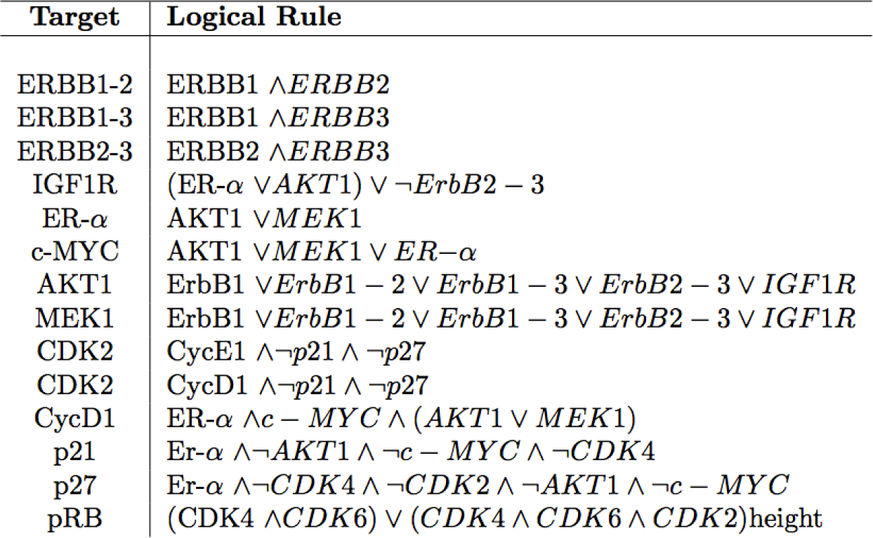
C. The ErbB Signaling Pathway

For this work, we used a Boolean model of the ErbB signaling pathway for the regulation of the G1/S cell cycle transition, as developed by [27]. In this article, the authors began by constructing a model from the literature, then proceeded to refine the model via network reconstruction. Although these refinements proved useful in the selection of novel targets for gene therapy, we would like to focus on the initial derivation of the model in which all reactions correspond to cited regulations. However, we will use the logical rules suggested within this article for the refinement of the process hitting model via cooperative sorts, shown in Figure 9. All of the reaction rates were set to one.
EGF (epidermal growth factor) binds to ErbB receptors, of which there are four structural variants, three thought to be involved in this network. These receptors are functional when they form heterodimers, excluding ErbB1, which is able to function as a homodimer, as well. Functional receptors transmit signals to AKT1, an apoptosis-inhibiting transmitter, and MEK1, a protein kinase. Along with transcription factors c-MYC and ER-α, these entities downregulate kinase inhibitors p21 and p27, while upregulating the cyclins (CycE1 and CycD1) needed to activate their respective cyclin-dependent kinases (CDK). These CDKs will work to phosphoralize, and, therefore, inactivate, the retinoblastoma protein (pRB). Only when this protein is inactive can the E2F group of transcriptional factors required for DNA replication and, therefore, cell proliferation be activated. Although the interaction between CDKs and pRBs is inhibitive, we have kept the activations as indicated by the authors, using pRB as a proxy for its following and more interesting product, E2F. In addition, we have included the logical rule proposed for cyclin D presented in their work.

Acknowledgments

The authors acknowledge the contribution of Courtney Chancellor, who participated during one year to this research activity, and the first author, Francisco Chinesta, acknowledges the support of the Institute Universitaire de France (IUF). The work of Elias Cueto and Francisco Chinesta has been partially funded by the Spanish Ministry of Economy and Innovation through Grant Number DPI2014-51844-C2-1-R.

Author Contributions

Francisco Chinesta, Amine Ammar and Elias Cueto were in charge of the efficient treatment of the chemical master equation, whereas Morgan Magnin and Olivier Roux developed the qualitative modeling and its probabilistic counterpart. All authors have read and approved the final manuscript.

Conflicts of Interest

The authors declare no conflict of interest.
PACS classifications: 02.60.-x; 02.50.Ga; 87.18.-h

References

  1. Gillespie, D.T. Exact stochastic simulation of coupled chemical reactions. J. Phys. Chem. 1977, 81, 2340–2361. [Google Scholar]
  2. Gillespie, D.T. Approximate accelerated stochastic simulation of chemically reacting systems. J. Chem. Phys. 2001, 115, 1716–1733. [Google Scholar]
  3. Hegland, M.; Burden, C.; Santoso, L.; MacNamara, S.; Boothm, H. A solver for the stochastic master equation applied to gene regulatory networks. J. Comput. Appl. Math. 2007, 205, 708–724. [Google Scholar]
  4. Hasty, J.; McMillen, D.; Isaacs, F.; Collins, J.J. Computational studies of gene regulatory networks: in numero molecular Biology. Nature Rev. Genet 2001, 2, 268–279. [Google Scholar]
  5. Munsky, B.; Khammash, M. The finite state projection algorithm for the solution of the chemical master equation. J. Chem. Phys. 2006, 124/4, 044104. [Google Scholar]
  6. Sasai, M.; Wolynes, P.G. Stochastic gene expression as a many-body problem. Proc. Natl. Acad. Sci. 2003, 100, 2374–2379. [Google Scholar]
  7. Sreenath, S.N.; Cho, K.H.; Wellstead, P. Modeling the dynamics of signalling pathways. Essays Biochem. 2008, 45, 1–28. [Google Scholar]
  8. Kim, K.Y.; Wang, J. Potential energy landscape and robustness of a gene regulatory network: toggle switch. PLoS Comput. Biol. 2007, 3, 0565–0577. [Google Scholar]
  9. Priami, C.; Regev, A.; Shapiro, E.; Silverman, W. Application of a stochastic name-passing calculus to representation and simulation of molecular processes. Inf. Process. Lett. 2001, 80, 25–31. [Google Scholar]
  10. Ammar, A.; Cueto, E.; Chinesta, F. Reduction of the Chemical Master Equation for Gene Regulatory Networks Using Proper Generalized Decompositions. Int. J. Numer. Methods Biomed. Eng. 2012, 28, 960–973. [Google Scholar]
  11. Andreychenko, A.; Mikeev, L.; Wolf, V. Reconstruction of multimodal distributions for hybrid moment-based chemical kinetics. J. Coupled Syst. Multiscale Dyn. 2014, arXiv, 1410.3267. [Google Scholar]
  12. Kauffman, S.A. Metabolic stability and epigenesis in randomly constructed genetic nets. J. Theor. Biol. 1969, 22, 437–467. [Google Scholar]
  13. Thomas, R. Regulatory networks seen as asynchronous automata: a logical description. J. Theor. Biol. 1991, 153, 1–23. [Google Scholar]
  14. Pauleve, L.; Magnin, M.; Roux, O. Tuning temporal features within the stochastic π-calculus. IEEE Trans. Softw. Eng. 2011, 37, 858–871. [Google Scholar]
  15. Folschette, M.; Pauleve, L.; Magnin, M.; Roux, O. Under-approximation of reachability in multivalued asynchronous networks. Elect. Notes Theor. Comput. Sci. 2013, 299, 33–51. [Google Scholar]
  16. Pauleve, L.; Magnin, M.; Roux, O. Refining dynamics of gene regulatory networks in a stochastic π-calculus Framework. In Transactions on Computational Systems Biology XIII; Springer: Berlin/Heidelberg, Germany, 2011; pp. 171–191. [Google Scholar]
  17. Ammar, A.; Mokdad, B.; Chinesta, F.; Keunings, R. A new family of solvers for some classes of multidimensional partial differential equations encountered in kinetic theory modeling of complex fluids. J. Non-Newtonian Fluid Mech. 2006, 139, 153–176. [Google Scholar]
  18. Ammar, A.; Mokdad, B.; Chinesta, F.; Keunings, R. A new family of solvers for some classes of multidimensional partial differential equations encountered in kinetic theory modeling of complex fluids. Part II: transient simulation using space-time separated representations. J. Non-Newton. Fluid Mech. 2007, 144, 98–121. [Google Scholar]
  19. Chinesta, F.; Ammar, A.; Falco, A.; Laso, M. On the reduction of stochastic kinetic theory models of complex fluids. Model. Simul. Mater. Sci. Eng. 2007, 15, 639–652. [Google Scholar]
  20. Chinesta, F.; Ammar, A.; Joyot, P. The nanometric and micrometric scales of the structure and mechanics of materials revisited: An introduction to the challenges of fully deterministic numerical descriptions. International. J. Multiscale Comput. Eng. 2008, 6, 191–213. [Google Scholar]
  21. Kazeev, V.; Khammash, M.; Nip, M.; Schwab, C. Direct Solution of the Chemical Master Equation Using Quantized Tensor Trains. PLoS Comput. Biol. 2014, 10/3, e1003359. [Google Scholar] [CrossRef]
  22. Ammar, A.; Chinesta, F.; Diez, P.; Huerta, A. An error estimator for separated representations of highly multidimensional models. Comput. Methods Appl. Mech. Eng. 2010, 199, 1872–1880. [Google Scholar] [Green Version]
  23. Chinesta, F.; Ammar, A.; Leygue, A.; Keunings, R. An overview of the proper generalized decomposition with applications in computational rheology. J. Non-Newton. Fluid Mech. 2011, 166/11, 578–592. [Google Scholar]
  24. Chinesta, F.; Keunings, R.; Leygue, A. The Proper Generalized Decomposition for advanced numerical simulations. A primer. In Springer Briefs in Applied Sciences and Technology; Springer: Heidelberg, Germany, New York, NY, USA, Dordrecht, The Netherlands, London, UK, 2014. [Google Scholar]
  25. Chinesta, F.; Ammar, A.; Cueto, E. Recent advances and new challenges in the use of the proper generalized decomposition for solving multidimensional models. Arch. Comput. Methods Eng. 2010, 17, 327–350. [Google Scholar]
  26. Chinesta, F.; Ladeveze, P.; Cueto, E. A short review on model order reduction based on proper generalized decomposition. Arch. Comput. Methods Eng. 2011, 18, 395–404. [Google Scholar]
  27. Sahin, O.; Frohlich, H.; Lobke, C.; Korf, U.; Burmester, S.; Majety, M.; Mattern, J.; Schupp, I.; Chaouiya, C.; Thierry, D.; Poustka, A.; Wiemann, S.; Beissbarth, T.; D. Arlt, D. Modeling erbb receptor-regulated g1/s transition to find novel targets for de novo trastuzumab resistance. BMC Syst. Biol. 2009, 3. [Google Scholar] [CrossRef]
  28. Folschette, M.; Pauleve, L.; Inoue, K.; Magnin, M.; Roux, O. Concretizing the process hitting into biological regulatory networks. In Computational Methods in Systems Biology; Gilbert, D., Heiner, M., Eds.; Lecture Notes in Computer Science; Springer: Berlin/Heidelberg, Germany, 2012; pp. 166–186. [Google Scholar]
  29. Chinesta, F.; Leygue, A.; Bordeu, F.; Aguado, J.V.; Cueto, E.; Gonzalez, D.; Alfaro, I.; Ammar, A.; Huerta, A. PGD-based computational vademecum for efficient design, optimization and control. Arch. Comput. Methods Eng. 2013, 20/1, 31–59. [Google Scholar]
  30. Mangan, S.; Alon, U. Structure and function of the feed-forward loop network motif. PNAS 2003, 21, 11980–11985. [Google Scholar]
Figure 1. Creating a process hitting action. In gene regulation, we consider two kinds of interactions between species: activation and inhibition. If a is an activator of b, it is common to represent this by a signed, directed graph (left). These interactions have a characteristic form: unlike kinetic reactions, activation and inhibition usually depend on the regulator passing some threshold concentration in order to become effective (middle). Process hitting (right) represents these reactions via actions: a activates b becomes a1 hits (solid arrow) b0 to bounce (dashed arc) to b1. Generalized dynamics attempts to create the most permissive dynamics possible for the directed graph. Therefore, the absence of a effectively acts as an inhibitor, adding the action a0 hits b1 to bounce to b0. Every action can be associated with temporal and stochastic parameters; the reaction rate, for example [14].
Entropy 17 01896f1
Figure 2. Refinement of a model via cooperative sorts. Here, a is an activator of c, while b inhibits c. The generalized dynamics of the system have been constructed on the left. However, what should happen in the case that both and are present? According to the left-hand model, the system will oscillate. If we know more about how the system should function, however, we would like to be able to include this information in our model. With general dynamics, we are unable to express logical gates in which multiple species exhibit deterministic combined effects on a target, such as a ∧ −b, or the presence of the activator without the presence of the inhibitor. In order to add this combined interaction and eliminate the oscillatory behavior, we must refine the process hitting model with a cooperative sort, ab. This sort will handle the interactions of a and b on c, while leaving the original species to interact with other elements as before. In exchange, more actions must be added, such that a and b can effectively update ab, so that it truly reflects the current state of both elements. In our example, ab1,1 will not interact with c0; thus, c remains inactive.
Entropy 17 01896f2
Figure 3. Decomposition of a state space. This illustration shows how a multidimensional space, for example a cubic space of three dimensions involving 33 degrees of freedom, can be decomposed into the product of the individual dimensions, 3 · 3. This mathematical property is exploited by PGD in that we search for the individual vectors, which are of a relatively small size, never touching the full state space. In such a way, we move from a complexity of Kn to K · n.
Entropy 17 01896f3
Figure 4. Sample of the results from incorporating model parameters as dimensions in the PGD solution. Here, we have selected three potential values for the firing rate r: r/2 (left), 3r/2 (middle) and 2r (right), for any interaction involving the proteins p21 or p27. The resulting behaviors of five proteins along the chemical pathway are shown here. Since the system is binary, active expression is plotted in yellow and inactive in blue, following their probabilities on the y-axis. Notice that in all cases, behavior is equivalent until around 1.75 seconds, when the firing cascade reaches p21 and p27. Some signals are simply amplified, whereas others, such as p21 and pRB, develop more complicated behaviors as the firing rate increases, perhaps suggesting cyclical or dampening behaviors.
Entropy 17 01896f4
Figure 5. Interaction graph of the incoherent feed-forward loop.
Entropy 17 01896f5
Figure 6. (a) Generalized Boolean dynamics of the incoherent feed-forward loop in process hitting. (b) Possible transitions from the state (a1, b0, c0).
Entropy 17 01896f6
Figure 7. Refined process hitting encoding the dynamics of the incoherent feed-forward loop where the activation of c needs both a inactive and b active. The process 01 of the sort ¬ab mirrors the (only) state where c0 should be hit. Grayed processes indicate the initial state for the transition graph in Figure 8.
Entropy 17 01896f7
Figure 8. Transition graph of the process hitting in Figure 7 from the state represented by grayed processes.
Entropy 17 01896f8
Figure 9. The proposed logical rules for species with more than one regulator.
Entropy 17 01896f9
Figure 10. The interaction graph for ErbB-mediated G1/S cell cycle transition. Here, elements directly related to the ErbB signaling portion of the network are represented by boxes, while the elements related to kinase activity are represented by circles. Activation interactions are shown in green arrows and inhibition in red blunted arrows. Since this is the initial, most basic network derived from the literature, no combined effects requiring Boolean logic gates are shown.
Entropy 17 01896f10
Table 1. Results for ErbB models using generalized dynamics and a refinement with cooperative sorts. Here, the two models were tested using three sanity checks related to our biological understanding of the system: the presence of fixed points, the lack of impossible behaviors and the presence of demonstrated behaviors. In order to be considered a functioning model, pRB should remain at rest when the system is universally inactive, including the absence of input protein EGF. However, in the presence of EGF, a signal should be able to propagate through the system, potentially activating pRB. We see that, while the generalized dynamics were able to propagate a signal from EGF to pRB (EGF present), it was not able to prevent sporadic activation of pRB in a system at rest (EGF absent), nor find any fixed points.
ModelFixed pointsEGF absentEGF present
Gen. Dynam.0FailPass
Refined3PassPass

