Computer Simulations of Soft Matter: Linking the Scales

Abstract

In the last few decades, computer simulations have become a fundamental tool in the field of soft matter science, allowing researchers to investigate the properties of a large variety of systems. Nonetheless, even the most powerful computational resources presently available are, in general, sufficient to simulate complex biomolecules only for a few nanoseconds. This limitation is often circumvented by using coarse-grained models, in which only a subset of the system’s degrees of freedom is retained; for an effective and insightful use of these simplified models; however, an appropriate parametrization of the interactions is of fundamental importance. Additionally, in many cases the removal of fine-grained details in a specific, small region of the system would destroy relevant features; such cases can be treated using dual-resolution simulation methods, where a subregion of the system is described with high resolution, and a coarse-grained representation is employed in the rest of the simulation domain. In this review we discuss the basic notions of coarse-graining theory, presenting the most common methodologies employed to build low-resolution descriptions of a system and putting particular emphasis on their similarities and differences. The AdResS and H-AdResS adaptive resolution simulation schemes are reported as examples of dual-resolution approaches, especially focusing in particular on their theoretical background.

1. Introduction

Since the pioneering work carried out by Berni Alder [1] in the 1950s, in silico experiments, such as Molecular Dynamics (MD) or Monte Carlo (MC) simulations, allowed researchers to obtain major advancements in the understanding of systems with many degrees of freedom. In particular, during the last few decades, the increasing accuracy of the force-fields, the improvement of the algorithms, and the steady boost of computer power made it possible to perform insightful simulations of a broad variety of systems of increasing size and complexity, ranging from simple liquids -composed of idealized, point-like molecules interacting via simple potentials- to biomolecules. Nonetheless, the amount of available computational resources can be insufficient to simulate, for a physically meaningful time, even the simplest nontrivial macromolecule. It is often the case, in fact, that “interesting” phenomena in these systems occur on very long time-scales: a simple example of this is provided by the diffusion of a polymer in a melt [2,3]; the same behavior can observed in conformational changes of proteins [4–9], at least in those cases in which the force field provides a good approximation to the real atomistic interactions.

At the same time, in many cases the massive amount of data that are produced in a simulation is composed mostly of non-useful information. A prototypical example is given by the solvent: the water molecules that solvate a protein or a membrane are typically discarded from the analysis that follows the simulation, with the possible exception of a few solvation shells around the molecule itself. In this case a large fraction of the computational power is employed in the integration of the equations of motion of degrees of freedom which are extremely relevant during the simulations, but are completely neglected afterwards.

In order to overcome this limitation, coarse-grained models [10–15] have been developed, where the structure and interactions of the original system are replaced with simpler ones, which are easier to describe, model, simulate and understand. The assumption underlying the coarse-graining of a system is that above a given length scale the low-level, chemistry-specific detail of the model affects some properties of the system only in a simple, functionally trivial way - often through prefactors. Examples of systems for which this approach proved to be extremely successful are molecular fluids, polymers [2,3,16,17], elastic network models of proteins [18–23], lipid membranes and other biomolecular systems, just to mention a few.

In recent years, systematic coarse graining approaches have gained importance, where the interactions in the coarse-grained (CG) model are derived systematically from atomistic reference simulations in a bottom-up fashion. These models are often used in a multiscale simulation framework, where the closeness of higher and lower levels of resolution allows a switching back and forth between them. Below, we will review several systematic coarse graining approaches and address some of the most important methodological issues and challenges.

The smaller amount of degrees of freedom that are retained in coarse-grained models and the simpler force-fields employed allow the characterization of relevant properties of a system at a cheaper computational cost compared to the high-resolution atomistic models; on the other hand, there are cases in which the chemical detail in a small region of the system plays a crucial role, such that no simplification of the description is possible: think, for example, of the active site of a large enzyme, where fine-grained chemical processes take place. A high-resolution modeling of each part of the system would not be necessary, but at the same time a coarse-graining approach would delete important information.

This last observation naturally leads us to identify a particular class of soft matter systems among those that are studied with the help of computer simulations. Specifically, we can consider those systems where the focus is on a small, well-defined subregion of the simulation box. To this class belong, for example, certain solvated (macro)molecules, active sites of enzymes, the interaction of specific polymer ends at a surface, or simply a small spherical region in a homogeneous fluid whose radius is of the length scale of the property we are interested in.

For such systems the remaining, “non-interesting” region consists of the volume containing all those degrees of freedom which will be eventually neglected and/or discarded once the simulation is done, such as the solvent or large parts of a macromolecule which do not play an active role in the process of interest (e.g., all atoms sufficiently far from the active site of an enzyme). Usually, detailed knowledge about structural, energetic and thermodynamical properties of these large sections of the system is not required; nonetheless these “non-interesting” degrees of freedom have to be explicitly present and integrated, inasmuch as they “scaffold” the target object of the simulation and represent a reservoir of energy and molecules.

A method is thus required that allows one to perform a simulation where the largest part of the computational resources is concentrated on that region of the system that will be subsequently analyzed. Adaptive resolution simulations methods [24–34] were developed to solve the contradiction between the necessity of simulating all parts of the system and the fact that, eventually, the detailed information from a large subgroup of them will be neglected. The underlying idea is to replace these “non-interesting” degrees of freedom of the system with a simpler, coarse-grained representation, such that a sensibly smaller number of computations (e.g., force calculations) is required, while the “interesting” region is treated at a higher resolution.

This approach gives rise to at least two important conceptual problems that have to be solved:

(1)

what is the smallest number of properties of the original system that have to be retained in the coarser model, and which are they;

(2)

how to interface the low-resolution, “non-interesting” region and the high-resolution region to preserve the correct physics at least in the latter.

These two problems are obviously interconnected, since the way the high- and low-resolution regions interact at the interface naturally depends on the specific properties of the models used in each of them; a thorough discussion of these aspects will be carried out in the context of the Adaptive Resolution Simulation (AdResS) [24–32] and Hamiltonian AdResS [33,34] (H-AdResS) methods.

The present review is composed of two principal parts: in Section 2 the basics of coarse-graining theory are presented together with a few examples of the most commonly used techniques, e.g., Force Matching, Boltzmann Inversion and Relative Entropy; in Section 3 we discuss two strategies, the adaptive resolution simulation (AdResS) scheme and the Hamiltonian AdResS (H-AdResS) to perform simulations in which different regions of the same system are modeled with different resolution.

Large parts of the present review are based on course material that was compiled for two workshops at the Forschungszentrum Jülich (“Hierarchical Methods for Dynamics in Complex Molecular Systems, 2012” [35], and “Workshop on Hybrid Particle-Continuum Methods in Computational Materials Physics”, 2013 [36]), as well as on original publications on the respective methodologies [33,34,37–40].

2. Coarse-Graining

As was mentioned in the Introduction, there are many interesting physical problems for which a detailed description of the system at the all-atom (AA) level is not necessary to obtain the relevant information. In these cases a simpler model might be used, where a given high-resolution, computationally expensive model is replaced with a simpler one.

These Coarse-Grained models possess a number of features that make them particularly appealing. For example, a smaller amount of computational resources is required to perform a simulation: this is due to both the reduced number of degrees of freedom and the simpler form of the interactions. Another important characteristic is that since many interaction centers are replaced with a single one, the fluctuations of the force experienced by a molecule are generally much smaller; this results in smoother free energy profiles and, as a consequence, in faster diffusive processes, allowing the system to reach larger time-scales with less computations. This last aspect implies that one typically has to determine a rescaling factor between the simulation timescale (usually given in Lennard Jones units) and the corresponding real world time (or the corresponding timescale in a higher resolution system). A detailed discussion of these dynamic aspects with further references can be found in Reference [41]. Finally, coarse-grained models are designed to reproduce large length-scale properties of the system, such as the global, collective conformational changes of a protein or the diffusive process of a polymer in a melt, that can be strongly insensitive to the fine-grained, chemistry-specific details; as a consequence, the parametrization of the coarse-grained interactions is also advantageously simpler.

Many CG models are generic, i.e., they were not developed to model a specific chemical system but rather with the aim of studying a physical phenomenon such as folding or aggregation in general. One example is generic CG lipid models, which have been successfully employed to study the self assembly of micelles, bilayers and other structures [42–46]. Generic CG models have also been employed to study folding and aggregation of peptides and proteins [47–59]. For polymers, such generic models were especially successful. Following the so called 1/N theorem of de Gennes [60–62] it was shown that properties such as the overall chain extension as a function of the polymerisation index follow the same power law with the same exponent for all polymers, independent of the chemical species. The results of these scaling theories were instrumental in the development of generic and thus very efficient models, as well as in the interpretation of experiments. For dynamical properties generic models simulations provided the first direct evidence of the reptation/tube concept put forward by Edwards and de Gennes [63,64]. The reptation model is based on the fact that the dynamics of long polymer chains is dominated by the constraint that polymer chains cannot simply cut through each other.

A wide range of approaches have been developed that aim for consistency between a CG model and either experimental data or simulations of accurate high resolution models. Typically, these approaches are divided into thermodynamics-based and so-called structure-based ones. In thermodynamic coarse graining approaches, individual elements of the CG interaction function are separately parameterized based on thermodynamic reference data such as solvation free energies and partitioning data, liquid densities, surface tension, etc. [65–76]. (These are usually experimental reference data, but in a multiscale simulation approach the reference data can of course also be obtained from an atomistic simulation, to keep the CG and atomistic level thermodynamically consistent). In another group of approaches, one numerically generates CG interaction functions with the aim of reproducing the configurational phase space sampled in an atomistic reference simulation. These approaches may rely on different types of reference properties such as structure functions [77–89], mean forces [90–95] or relative entropies [96–98]. In the following subsection, a few basic notions of coarse-graining theory will be introduced, together with examples of the strategies that can be employed to perform the coarse-graining in practice.

2.1. The Mapping Function and the Potential of Mean Force

In a multiscale approach, one first needs to define the relationship between the two levels of resolution. This is typically done via mapping functions which determine the CG Cartesian coordinates of each site as a linear combination of coordinates for the atoms that are involved in the site (that could be via a center-of-mass or a center-of-geometry mapping or some other geometric construction). This means the CG coordinates R are constructed from the atomistic coordinates r via

$$\mathbf{R}=\mathbf{Mr}$$

(1)

where M is an n × N matrix (n and N being the number of particles in the atomistic and CG system, respectively). In the (canonical) sampling of the atomistic and CG systems with respective interaction potentials V^AA(r) and V^CG(R) the corresponding configuration functions P^AA(r) and P^CG(R) are given by

$$P^{AA}(\mathbf{r})=Z_{AA}^{-1}\hspace{0.17em}\text{exp}[-\beta V^{AA}(\mathbf{r})]$$

(2)

and

$$P^{CG}(\mathbf{R})=Z_{CG}^{-1}\hspace{0.17em}\text{exp}[-\beta V^{CG}(\mathbf{R})]$$

(3)

with Z_AA = ∫ exp[−βV ^AA(r)]dr and Z_CG = ∫ exp[−βV^CG(R)]dR being the respective partition functions and β = 1/k_BT. If one analyses the atomistically sampled system in CG coordinates one can determine the probability distribution of sampling atomistic coordinates that map to a given CG coordinate r)

$$P^{AA}(\mathbf{R})=\langle \delta (\mathbf{Mr}-\mathbf{R})\rangle$$

(4)

(Here, we follow the notation used by Noid and collaborators, e.g., in References [99,100]). The angular brackets indicate canonical sampling of the atomistic system (i.e., according to P^AA(r)). One can formulate the aim of many systematic coarse graining approaches in the following way: To sample the part of phase space which is sampled by the atomistic system with the same probability distribution. Following this, one possible definition of consistency between atomistic and CG level of resolution is that the two models are consistent if the canonical configurational distribution sampled by the CG model P^CG(R) is equal to the probability distribution P^AA(R) obtained after mapping the atomistic system to CG coordinates. In a canonical ensemble, independent degrees of freedom q are Boltzmann distributed and the Boltzmann inverse of P(q)

$$V(q)=-k_{B}T\hspace{0.17em}\text{ln\hspace{0.17em}}P(q)$$

(5)

is a many-dimensional potential of mean force (PMF), which, when used for example as an interaction potential in a CG simulation, reproduces the distribution P(q). This means that Boltzmann inversion of P^AA(R) defines, uniquely up to an additive constant, a high-dimensional CG potential

$$V_{PMF}^{CG}(\mathbf{R})=-k_{B}T\hspace{0.17em}\text{ln\hspace{0.17em}}{P}^{AA}(\mathbf{R})+const$$

(6)

which will result in a sampling of CG configurations consistent with the atomistic reference simulation. This high-dimensional, many-body CG potential contains both energetic and entropic contributions from the configurational sampling in the high-resolution model and the mapping between high-resolution and CG model (Equation (4)). Therefore, the resulting CG model is state point dependent and not necessarily readily transferable. While it is conceptually easy to formulate the PMF as a solution of the systematic coarse graining task, it is practically unfeasible. In most cases the PMF cannot be easily determined, and even if it were possible, the resulting high-dimensional potentials are computationally prohibitive. In addition, $V_{PMF}^{CG}(\mathbf{R})$ is a function of R, i.e., this PMF as is can in principle only be applied to a system which is identical in size to the atomistic reference system; if this limitation cannot be overcome, e.g., by breaking it down to short-range interactions, it would defeat the purpose of coarse graining. Therefore, one has to decompose the PMF into simpler independent terms and approximate it by simpler interaction functions, ideally ones that resemble interaction functions typically used in molecular mechanics forcefields, i.e., short range bonded contributions and pair potentials or similar. Conceptually, one can decompose the PMF into a series of many-body terms up to an N-body term, where N is the number of particles on the system. However, this itself does not solve the problem since these multi-body interactions are again computationally unfeasible.

$$\begin{array}{l}{V}_{PMF}^{CG}(\mathbf{R})=\sum _{i,j}{V}_2(r_{ij})+\sum _{i,j,k}{V}_3(r_{ij},r_{jk},r_{ik})+\cdots +const\\ \approx \sum _{i,j}{V}_{\text{eff}}(r_{ij})+const\end{array}$$

(7)

In Equation (7) one approximates the series by an effective pair interaction which also contains contributions from the higher order terms in Equation (7) (some approaches also include three-body terms for systems where this is necessary [101]). There are many approaches to this task of determining effective CG interactions, and all the resulting CG models are (only) approximations to $V_{PMF}^{CG}(\mathbf{R})$.

2.2. Multi-Scale Coarse-Graining

Probably the most painful limitation in the use of the many-body PMF is the fact that, in general, it cannot be decomposed into a sum of local contributions depending on the interactions between two to a few particles. A simple strategy would therefore be to decide a simple functional form of the potential, e.g., a sum of pairwise, radial interactions, which depend on a set of parameters; the values of the latter are then chosen so that the CG potential is as close as possible to the true PMF. This approach was pioneered by Ercolessi and Adams in 1994 [102] and Tschöp and coworkers in 1998 [103]. Later, Izvekov and Voth [104,105] made use of the force-matching concept of Ercolessi and Adams in the development of the Multi-Scale Coarse-Graining (MS-CG) method. These approaches have been successfully applied to a multitude of biomolecular and other soft matter systems, in particular to biomolecules [90–95].

The central idea of Force Matching is to use a variational (i.e., non-iterative) approach for constructing the CG potential based on the atomistic reference simulation (the recorded forces from the atomistic simulation). The numerical implementation of this variational principle works in such a way that the exact many-body PMF (Equation (6)) is represented by a linear combination of basis functions that are functions of the CG site coordinates [14,15]. For a given configuration of the CG coordinates, in fact, the average of the total atomistic force f_α acting on a CG site α is equal to the derivative of the many-body PMF:

$${\langle {\mathbf{f}}_{\alpha }\rangle }_{\mathbf{R}}\equiv -\frac{\partial U[\mathbf{R}]}{\partial {\mathbf{R}}_{\alpha }}$$

(8)

where the subscript R on the averages indicates that the sampling is constrained to those configurations of the AA system having the CG sites in a fixed configuration. The CG force field depends on M parameters g₁, ···, g_M, that can be prefactors of analytical functions, tabulated values of the interaction potentials, or coefficients of splines used to describe these potentials. These parameters have to be optimized so that the CG force field reproduces the forces in the atomistic system (after mapping) as close as possible. To this end, one minimizes the difference between the average AA force 〈f_Α〉_R and the force F_α due to the CG potential by minimizing the following quadratic function:

$${\chi }^2[\mathbf{F}]=\frac{1}{3N}\langle \sum _{\alpha =1}^N{\mid {\mathbf{f}}_{\alpha }-{\mathbf{F}}_{\alpha }\mid }^2\rangle$$

(9)

Equation (9) can be rephrased in terms of generalized scalar products of elements in a multi-dimensional vector space; these elements are the 3N-dimensional force-fields f and F acting on the CG sites, with the scalar product and the corresponding norm given by:

$$\begin{array}{l}{\mathbf{F}}^a·{\mathbf{F}}^b\equiv \langle \sum _{\alpha =1}^N{\mathbf{F}}_{\alpha }^a·{\mathbf{F}}_{\alpha }^b\rangle \\ \Vert \mathbf{F}\Vert \equiv \sqrt{\mathbf{F}·\mathbf{F}}\end{array}$$

(10)

Given the definitions in Equation (10), it can be shown that minimizing the function χ² in the MS-CG method is equivalent to minimizing the ‘distance’ between the many-body PMF and the CG potential:

$${\chi }^2[\mathbf{F}]={\chi }^2[{\mathbf{F}}^{\mathbf{PMF}}]+\frac{1}{3N}{\Vert {\mathbf{F}}^{\mathbf{PMF}}-\mathbf{F}\Vert }^2$$

(11)

The force-matching strategy thus projects the true many-body PMF onto the basis of functions that are used to define the CG force-field; a thorough formal explanation of this interpretation can be found in Reference [14,15].

It should be noted, however, that the CG force field is still an approximation to the high dimensional PMF within the limitations of the types of CG forces chosen (for example pair forces that can be derived either from analytical or from numerical tabulated potentials). This also implies that a CG model obtained from force matching does not by construction reproduce the pair correlation functions in the system, and the reproduction of local structural properties such as pair distributions may (or may not) be imperfect depending on the importance of cross-correlations between degrees of freedom. An exact reproduction of the underlying atomistic problem by matching mean forces therefore potentially requires the introduction of higher order (e.g., three-body) interactions. Noid and coworkers have extended the force matching method and demonstrated that the CG force field can be directly determined from structural correlation functions obtained from the atomistic system instead of the forces [99]. Their theoretical approach also allows an assessment of the correlations between different interactions that are neglected by straightforward Boltzmann inversion and allows the quantification of the importance of many-body correlations in CG models. In a recent study, Rudzinski and Noid explore these aspects in detail [106]. They demonstrate how the balance between accurately reproducing individual correlation functions (such as pair correlation functions or angle distributions) and also reproducing cross correlations between the respective degrees of freedom is affected by the mapping scheme and the coarse graining method (or more accurately its targets, namely the mean forces versus the individual correlation functions).

2.3. Boltzmann-Inversion Based Methods

In contrast to the Force Matching or Multi-scale coarse graining scheme, other structure-based methods provide CG interactions that reproduce pre-defined target structure properties—often a set of radial distribution functions [77–89]. This means that the many-body PMF (Equations (6) and (7)) is replaced as a target by a set of simpler structural correlation functions. If the interactions in the CG model are statistically independent or only weakly coupled then direct Boltzmann inversion determines each term in the potential immediately from the corresponding distribution function [77,107–109]; for non-bonded interactions in dense systems, though, this is typically not the case. This means that the individual distribution functions and their corresponding potentials of mean force, e.g., a radial distribution function of a simple liquid g_target(r) and its Boltzmann inverse, the pair PMF, $V_0^{CG}(r)=-k_{B}T\hspace{0.17em}\text{ln\hspace{0.17em}}{g}_{target}(r)$, cannot be directly used as an interaction function since they correspond not only to the interaction potential but also to the correlated contributions from the surroundings. These multi-body effects of the environment need to be removed from the PMF in order to generate an effective pair potential that reproduces the target structure, for example the pair correlation function in the liquid. It can be shown that such a pair potential is unique up to an arbitrary constant [110] and exists [96,111–113]. There are several numerical methods to generate this pair potential (tabulated interaction function).

Iterative Boltzmann inversion (IBI) [81,114,115] is a natural extension of the Boltzmann inversion method. Here, a numerical CG potential is iteratively refined until the target structure is reproduced within a predefined error. Each step in the iteration procedure is a CG simulation with potential $V_i^{CG}(r)$ which yields an RDF g_i(r) that differs from the target g_target(r). The potential is then modified by a correction term ΔV (r) according to

$$V_{i+1}^{CG}(r)=V_i^{CG}(r)+\mathrm{\Delta }{V}_i(r)=V_i^{CG}(r)+k_{B}T\hspace{0.17em}\text{ln}\frac{g_i(r)}{g_{target}(r)}$$

Sometimes the potential correction ΔV_i(r) is multiplied by a prefactor 0 < λ ≤ 1 to avoid overshooting in the numerical procedure. The iterative procedure is often initiated with the pair potential of mean force $V_0^{CG}(r)=-k_{B}T\hspace{0.17em}\text{ln\hspace{0.17em}}{g}_{target}(r)$, but that is not mandatory. Different starting potentials can be useful, in particular for more complex mixed systems where the iterative procedure may be unstable because intermediate CG models lead to phase separation. This is for example observed in the case of hydrophobic molecules in aqueous solution where both above-mentioned precautions have found to be useful to prevent strong oscillations or even instability of the IBI procedure.

IBI is by no means the only numerical method that solves the above task. Another numerical scheme is the so called inverse Monte Carlo (or more recently renamed Newton inversion) method [78,79,83,84] which, according to Henderson’s theorem, should lead to the same numerical solution for the pair potential corresponding to a given pair correlation function. While in IBI the potential update ΔV_i is ad hoc, in IMC it is computed using rigorous statistical mechanical arguments (for details see Reference [78]). In the case of multicomponent systems, where several pair potentials need to be updated, IMC accounts for correlations between observables, i.e., the updates for the different potentials are interdependent. In contrast, for IBI each potential is updated independently, which might lead to oscillations and convergence problems in the iteration procedure. The disadvantage of IMC on the other hand is a high computational cost and problems with numerical stability; for a detailed comparison see Reference [116]. Related to IMC, there are several other recent developments, e.g., a molecular renormalization group approach [85–87] or an approach that relies on relative entropies [96–98] (which will be discussed in more detail below). While the above structure-based methods by construction reproduce exactly, within the error of the numerical procedure, the local pair structures and thus are well-suited to the reinsertion of atomistic coordinates, it can be expected a priori that they will not be equally well suited to the reproduction of thermodynamic properties (pressure, phase behavior, etc.) of the reference system; in this respect, water provides a prototypical case and a reference for testing. Note also that CG models based on pair correlation functions do not necessarily reproduce higher-order (e.g., three-body) structural correlations [116] since the pair correlation functions as structural targets are just an approximation to the total conformational distribution function obtained from the atomistic sampling, P^AA(R) (Equation (4)). This means that if higher order correlations are a crucial part of the many-body PMF, models based on pair structures may fail to represent these, and it may even be possible that models which are limited to pair potentials may fail to reproduce these correlations irrespective of the parametrization methodology. One example where this is studied in detail is liquid water [101,116–119]. Recently Noid and coworkers have analyzed these aspects using concepts from liquid state theory [100,120].

One more note concerning Henderson’s theorem: even though there is in principle one exact solution for the effective pair potential that reproduces a given pair correlation function, different potentials might give a reasonably close representation of the structure, i.e., the above inverse problem is mathematically ill-posed [116,121].This effect becomes even more pronounced in complex systems where several interaction functions corresponding to several RDFs need to be numerically determined. This can to some extent be turned into an advantage since it allows one to impose thermodynamic constraints in the parametrization procedure. This will result in interaction functions which do not exactly reproduce the target structure but give a very close representation while at the same time producing the desired thermodynamic behavior. One example of this is pressure correction terms [81,117]. Here, an additional linear pressure correction is applied during the iterative Boltzmann inversion procedure with

$$\mathrm{\Delta }{V}_{i,P}^{CG}(r)=A_i\hspace{0.17em}\left(1-\frac{r}{r_{cut}}\right)$$

(12)

where r_cut is the radial cutoff distance of the non-bonded interaction and the constant A is determined via the virial expression for the pressure to

$$-\left[\frac{2\pi N\rho }{3r_{cut}}{\int }_0^{r_{cut}}{r}^3{g}_i(r)\text{d}r\right]\hspace{0.17em}{A}_i\approx (P_i-P_{target})\hspace{0.17em}V$$

(13)

V is the volume of the system, P_i the pressure of the CG model in the i-th iteration, and P_target the target pressure. The price to pay for this adjustment, however, is the loss of the perfect compressibility match. This phenomenon is of course a direct consequence of the state point dependency of coarse grained interactions. Further details on this topic can be found in Reference [117]. Recently, different functional forms of pressure correction terms and the influence of the cutoff length have been explored by Fu et al. [122].

It is to be expected that there will be more development in this direction (using other types of thermodynamic constraints) since in particular for complex soft matter system the balancing of structural and thermodynamic behavior in CG models is an ongoing field of research [88,89].

The IBI method is in its original form designed and best suited for systems with uniform density distributions. Recently, Jochum et al. have shown how it can be generalized for non-bonded potentials for inhomogeneous systems [123]. For a system with a slab geometry (such as systems of solvent slabs in vacuum or phase-separated systems consisting of two liquid slabs in contact with each other), the method is analogous to IBI but the iterative update of the interaction potential consists of two terms, one based on the radial distribution function calculated in a slab geometry and one that accounts for the slab and interfacial widths. These latter geometric features are very sensitive to the thermodynamic properties (surface tension) of the interface. Therefore the two update terms allow for a balance between the local liquid structure and the thermodynamic properties of the liquid/vapor or liquid/liquid interface. In addition to water/vapor and methanol/vapor interfaces, the method has also been successfully applied to a solute-solvent system of a single benzene molecule at the vacuum-water interface, i.e., it is possible to account to some extent for the partitioning behavior of a solute between bulk and interface, an aspect that makes this method promising in the context of designing transferable CG models for phase separation processes (see below).

Last but not least, one should mention the particular case of Boltzmann-inversion based approaches for mixed systems where (at least) one component is very dilute (from now on termed solute), e.g., biomolecules in aqueous solution. In this case, iterative Boltzmann inversion and similar methods are problematic. While one can easily compute the solvent-solvent and the solute-solvent radial distribution functions, and therefore determine the corresponding CG potentials with for example IBI, this is not so straightforward for the interactions between the low concentration component (solute). (Note that for simplicity only solutes that are represented by a single CG bead will be discussed here.) In these cases, obtaining the PMF through brute force sampling of a radial distribution function is not advisable. One should rather compute the solute-solute pair PMF (between two solute particles) with an advanced sampling method such as umbrella sampling or thermodynamic integration (using distance constraints) [124,125].

When solvent degrees of freedom are not explicitly present in the CG system, this solute-solute PMF can be used directly as an effective solute-solute non-bonded interaction since the environmental (solvent) effects within the PMF are not explicitly represented through solvent degrees of freedom in the CG model. For many types of solutes the solute-solute PMF has been used as an interaction potential in implicit solvent models [126,127]. One prominent example is the use of the solute-solute pair PMF for implicit solvent models of aqueous electrolyte solutions, i.e., implicit solvent ion models [37,79,85,128,129].

The case is somewhat different if some sort of explicit solvent representation, for example in the form of a CG water model, is present in the CG system. In this case, effective solute-solute non-bonded pair interactions are needed from which the solvent contributions are removed in the same way they are removed by IBI in other systems. However, due to the sampling problem of the PMF between dilute components, an iterative procedure is prohibitive for solute-solute interactions. To solve this problem, an approximate method has been developed by Villa et al. [38,130]. Here, the CG solvent-solvent and solute-solvent interactions are first determined, for example through normal IBI. Now the pair PMF between the solutes $V_{PMF}^{AA}(r)$ is computed (from atomistic umbrella sampling or thermodynamic integration) and used as a target, in other words the resulting CG model is parameterized to reproduce the solute-solute association strength observed in the atomistic system. In order to remove the solvent contribution from $V_{PMF}^{AA}(r)$, a subtraction procedure is employed. One conducts a separate PMF calculation (again with umbrella sampling or thermodynamic integration), this time in a CG system, where the (previously determined) CG solvent-solvent and solute-solvent interactions are present but no direct interaction between the solute particles is turned on. The resulting PMF $V_{PMF,excl}^{CG}(r)$ only consists of the environmental contributions (in the CG environment). By subtracting $V_{PMF,excl}^{CG}(r)$ from the target PMF one obtains the missing direct pair interaction

$$V^{CG}(r)=V_{PMF}^{AA}(r)-V_{PMF,excl}^{CG}(r)$$

(14)

which by construction reproduces the target PMF. Note that this subtraction procedure is not necessarily limited to CG solvent-solvent or solute-solvent interactions determined by IBI. In principle other types of CG solvent-solvent or solute-solvent interactions could also be used to determine $V_{PMF,excl}^{CG}(r)$

If one then applies Equation (14), one obtains an effective solute-solute interaction V^CG(r) which reproduces the atomistically observed solute-solute association strength (i.e., $V_{PMF}^{AA}(r)$) in the particular CG solvent that was chosen.

2.4. Relative Entropy

Aiming at reproducing different properties or objective functions of the reference, atomistic system, IBI and Force Matching have manifestly different algorithms and produce qualitatively different results. Recently a different coarse-graining strategy has been developed, namely the Relative Entropy method [131–133], which relies on a quantitative measure of the loss of information that follows from the description of a system in terms of different interaction potentials and/or different resolution. Remarkably, it is possible to demonstrate that the information function employed in this strategy connects Relative Entropy, IBI and Force Matching together. The functional form of this measure function is given by the relative entropy, or Kullback–Leibler distance:

$$S_{rel}=\sum _{\nu }{\mathcal{P}}_{AA}(\nu )·\text{ln\hspace{0.17em}}\left(\frac{{\mathcal{P}}_{AA}(\nu )}{{\mathcal{P}}_{CG}(\nu )}\right)$$

(15)

In Equation (15), ν labels a given microstate or atomistic configuration, ℘_AA(ν) is the probability of sampling a configuration ν in the fully atomistic system, and ℘_CG(ν) is the probability of sampling the same (atomistic) configuration in the system with coarse-grained interactions, but still described by a high-resolution structure. This latter probability is degenerate with respect to the atomistic-potential configurations, as many of them correspond to the same coarse-grained configuration . It is therefore advantageous to write the probability to sample a given atomistic configuration in the CG system in terms of the function that maps the fine-grained configurations onto the coarse-grained ones:

$$\begin{array}{l}{\mathcal{P}}_{CG}(\nu )\equiv \frac{{\mathcal{P}}_{CG}^{\prime }(\mathcal{V})}{\mathrm{\Omega }(\mathcal{V})}\\ \mathcal{V}\equiv \text{M}(\nu )\end{array}$$

(16)

Here, ${\mathcal{P}}_{CG}^{\prime }(\mathcal{V})$ is the probability of sampling the CG configuration in the low-resolution system and Ω( ) = ∑_ν δ(M(ν) − ) is a measure of the degeneracy of the configuration in the atomistic system. It should be noted that this last quantity depends only on the mapping function M and not on the coarse-grained interactions; this term can therefore be separated out in the definition of the relative entropy to obtain:

$$\begin{array}{l}{S}_{rel}=S_{map}+\langle \phi \rangle \\ \text{with}:\\ \langle \mathcal{Q}\rangle \equiv \sum _{\nu }{\mathcal{P}}_{AA}(\nu )·\mathcal{Q}(\nu )\end{array}$$

(17)

$$\begin{array}{l}{S}_{map}=\langle \text{ln\hspace{0.17em}}(\mathrm{\Omega }(\mathbf{M}(\nu )))\rangle \\ \phi (\nu )=\text{ln\hspace{0.17em}}\left(\frac{{\mathcal{P}}_{AA}(\nu )}{{\mathcal{P}}_{CG}(\mathbf{M}(\nu ))}\right)\end{array}$$

(18)

The quantity φ(ν) can be interpreted as the amount of information in the configuration ν which discriminates between the atomistic and the coarse-grained probability. The definition in Equation (17) is particularly appealing because it shows that the relative entropy can be computed as the sum of operator averages. In the special, but quite common case of systems in thermal equilibrium, the probability distributions ℘ are simply given by the Boltzmann weights, and the relative entropy reduces to the form:

$$S_{rel}=S_{map}+\beta [(A_{AA}-A_{CG})-{\langle U_{AA}-U_{CG}\rangle }_{AA}]$$

with A_AA (resp. A_AA) being the free energy of the atomistic (resp. CG) system. For a given choice of the mapping function M, the optimal coarse-grained potential is obtained by minimizing the relative entropy functional with respect to the parameters in terms of which the aforementioned potential is defined: common choices for non-bonded, two-body interactions are the coefficients of a Lennard-Jones potential or the nodes of a spline.

As anticipated at the beginning of this section, IBI and Force Matching can be connected using the concept of relative entropy. In fact, a straightforward minimization of S_rel making use of two-body coarse-grained potentials can be shown to be equivalent to the IBI algorithm; on the other hand, the Force Matching scheme is retrieved if the average of the function |∇φ|² is minimized instead of the average of φ [134]: the squared gradient of the φ function with respect to the Cartesian coordinates, in fact, is proportional to the squared difference of the forces obtained from the AA and the CG descriptions, so that:

$${\chi }^2[\mathbf{F}]={\chi }^2[{\mathbf{F}}^{\mathbf{PMF}}]+\frac{{(k_{B}T)}^2}{3N}\langle {\mid \nabla \phi \mid }^2\rangle$$

(19)

In conclusion, it therefore appears evident that different coarse-graining schemes are obtained through the minimization of different functionals of the same information function φ, which represents the unifying element between various approaches.

2.5. Transferability of Coarse-Grained Models

From the preceding sections we have seen that there are different approaches to the systematical parameterization of CG models which by construction will not be equally well suited to the reproduction of thermodynamic and structural properties of the system. It is not a priori clear whether structure-based potentials reproduce macroscopic thermodynamic properties and, vice versa, if thermodynamics-based potentials reproduce microscopic structural properties. However, the interplay of structure and thermodynamics is crucial for the investigation of structure formation processes, in particular for biomolecular aggregation in aqueous solution where partitioning and phase separation play a decisive role. All CG models (in fact also all classical atomistic forcefields) are state-point dependent and cannot necessarily be—without reparametrization—transferred to different thermodynamic conditions or a different chemical environment compared to the one where they had been derived. This means “transferability” can refer to a change in temperature, density, concentration, system composition, phase, etc., but also a change in chemical environment, e.g., the change of length or sequence of an amino acid chain. Structure-motivated CG models which approximate the high dimensional PMF obtained from an atomistic reference are by construction heavily state point dependent, and several studies have addressed questions regarding their ability to reproduce thermodynamic properties. One system that has been of particular interest in this context is liquid water [112,117,135]. The reason is on the one hand of course its immense importance in all questions regarding biomolecular systems. In addition, it is of particular methodological interest because for single bead models of water it is known that three-body correlations play a decisive role and the potential compromise between reproducing pair- or higher order structural correlations is particularly relevant for the properties of the model [101,116,117]. Different studies have been carried out that compare structure-motivated and thermodynamics-based CG models [121,136,137]. While CG models where the parametrization targets had been solvation and partitioning properties are particularly well suited to reproduce processes where for example hydrophilicity/hydrophobicity arguments play a decisive role, they do not per se reproduce the structure of the system [121,136]. Related to their ability to reproduce the thermodynamic properties of certain chemical units, these models exhibit considerable transferability and can often be applied to a variety of molecular systems and a range of thermodynamic conditions. Motivated by these observations, intensive research is currently being carried out to derive CG potentials that are both thermodynamically as well as structurally consistent with the underlying higher-resolution description, thus ensuring for example a certain state point transferability [38,88,89,94,138].

One possibility to improve transferability in this context is to exploit—similar to the case of the pressure correction described above—the fact that the derivation of a CG model based on the reproduction of structural properties (potentials of mean force) is an ill-posed problem which allows a reproduction of the original target property within a given error while at the same time including certain thermodynamic target properties during parametrization. One approach developed by Ganguly et al. for multicomponent systems that follows this idea combines the IBI method with Kirkwood–Buff integrals as additional targets which are related to the activity coefficients of the components [139]. With this approach transferability over a certain concentration range can be achieved.

Yet another non-structure-based method that produces CG pair potentials with remarkable state point transferability is the conditional reversible work method by Brini et al. [140–142]. Here, several calculations of pair potentials of mean force on the atomistic level are used to assess and correctly account for the indirect contribution by the environment to the effective CG pair forces. The observed transferability of this method can be ascribed to the fact that the method relies on direct pairwise interactions in the atomistic reference system. In other words, the method does not rely on reproducing a structural property such as a pair PMF or multi-body PMF, i.e., on properties that are extremely dependent on the precise thermodynamic state of the reference system.

It has been mentioned before that effective pair potentials account for multi-body effects, for example, three body interactions. For this reason, they are only to a limited extent additive, which limits the transferability of the potentials [38,143]. Understanding the physical nature of non-additivity in the system of interest can help to make a CG model transferable. In principle, there are various possibilities to approach the question of transferability of effective pair potentials: (i) One applies a model derived at/optimized for a given state point unaltered to a range of state points nearby; in that case, one has to carefully investigate the range in which this is permitted [144–146]; (ii) One creates a new set of potentials for each state point one wants to investigate [144]; (iii) One specifically designs a single CG model with the aim of transferability (for example specific density dependent potentials [94,147,148], CG models that are designed to be applicable for a range of mixture compositions [71,138], or CG models that are capable of capturing a liquid crystalline phase transition [88,89]); (iv) One uses a model derived at one state point and (analytically) modifies it to be applicable to different conditions (one example being the rescaling of potentials in order to apply them to a different temperature [149]).

The approach of using a model at a specific state point and then testing its transferability over a reasonably wide range of different physical conditions has traditionally been applied in the case of classical polymer melts. In this field, structure-based models have been very successfully applied, and decent temperature [77,150–152] and pressure transferability [153] have been found. In fact in the first papers by Tschöp et al. [77,103] the temperature transferability already allowed the semi-quantitative prediction of shifts in Vogel Fulcher temperature for different polycarbonate modifications. This observation appears to hold for classical isotropic polymer melt systems where the behavior is largely dominated by the correct representation of the chain conformations and the excluded volume of the chain. As soon as more specific chemical interactions play a role, the case of transferability becomes more delicate.

In the following, we discuss three examples which illustrate that understanding the physical basis behind the limitations in transferability can help to design transferable models.

Binary mixtures have in general been widely used as model systems to explore various aspects of the transferability of CG models [37,38,71,128,129,138,143,147,148]. The transferability to different concentrations of liquid mixtures or solutions is of vital importance for simulation of processes such as (bio)molecular aggregation which are characterized by spatially varying structure and fluctuating concentrations.

Following the above-described method to apply Boltzmann-inversion derived methods in dilute solute solvent systems, a CG model for mixed systems of benzene in water had been derived [38]. This means that the CG benzene-benzene potential had been parameterized on the basis of the benzene-benzene PMF of two benzene molecules in aqueous solution, i.e., at “infinite” dilution. Benzene-water mixtures of different composition have been studied with this CG model and analyzed using the Kirkwood-Buff theory of solutions [154]. Kirkwood-Buff theory provides a link between local structural information and thermodynamic properties of the solution. This CG model, parametrized at infinite dilution of benzene, reproduces the Kirkwood-Buff integrals of mixtures at various concentrations obtained with the detailed-atomistic model. It reproduces the changes in the benzene chemical potential and the activity coefficients of the mixtures over a range of mixture compositions (up to concentrations where benzene and water demix in the atomistic reference simulation). A possible explanation is that hydrophobic interactions between benzene solutes are short-ranged, and the multi-body correlations involved in hydrophobic association can be described by pairwise additive effective potentials (category (i) of the above list). The observed transferability of the potential supports the idea that hydrophobic interactions between small molecules are pairwise additive. Villa et al. also found that a different CG model for benzene-benzene interactions that had been derived for pure benzene (via IBI) is neither suited to describe benzene-benzene interactions in aqueous solution at different concentrations nor a phase-separated benzene/water system with a bulk benzene layer [38].

To reproduce the actual phase separation process as well as the behavior of the mixed (or dilute) systems is much more complicated (yet it is of vital importance in the parameterization of bottom-up CG models that are able to reproduce biological partitioning and self aggregation phenomena). Here, a combination of a wise choice of one or possibly several reference state points is promising, in particular combining the reference of infinite dilution with the phase separated one. For the latter, application of the IBI extension by Jochum et al. for inhomogeneous systems with an interface/phase boundary can be utilized [123].

In this context it should also be mentioned that similar transferability problems exist in other areas, for example in the simulations of solids (e.g., with embedded atom potentials). As soon as one encounters surfaces or interfaces the local environment of an atom differs substantially from the bulk (crystalline) phase, which was used to parameterize the interaction potentials. Consequently the transferability of the potentials will affect the ability to model processes such as crack formation or the relocation of grain boundaries [155,156].

In the second example, the situation is different. Here, the transferability of CG (in this case implicit-solvent) ion models in aqueous solution had been investigated. Due to long-range electrostatic interactions, the ions affect the behavior of water increasingly strongly with increasing ion concentration. More specifically, the presence of many ions reduces the orientational fluctuations of the water molecules and thus the dielectric permittivity of the solvent. Therefore, effective ion-ion potentials parametrized at infinite dilution are not directly transferable to higher salt concentrations. Hess et al. developed a reduced-resolution (in this case implicit-solvent) potential for aqueous electrolyte solutions where an ion-concentration-dependent Coulomb term was added to the (ion-specific) pair interaction. Thus, by using a concentration-dependent dielectric permittivity for water, part of the multi-body effects in the system were accounted for in the ion-ion pairwise interaction in the implicit solvent model [128,129]. This approach reproduced the NaCl solution osmotic properties and the ion coordination up to a concentration of 2.8 M (mol/L). While in the case of the CG model of benzene/water mixtures [38] the short-range hydrophobic interactions parameterized at infinite dilution were directly transferable to higher benzene concentrations, the ion-ion interactions determined at infinite dilution had to be split into a short-range ion-specific and a long-range electrostatic part. The interactions were then made transferable by keeping the short-ranged part constant and analytically modifying the long-ranged electrostatic part (category (iv) of the above list). Shen et al. have further investigated the structure and osmotic properties of electrolyte solutions over a wide range of concentrations [37]. Using a concentration-dependent dielectric constant one also obtains very good structural properties of the electrolyte solution at low and intermediate salt concentrations while for larger salt concentrations multi-body ion-ion correlations limit straightforward transferability. Guided by this structural analysis, the transferability of the implicit-solvent model could also be improved for high ion concentrations. One obtains transferable implicit-solvent effective pair potentials which are both structurally and thermodynamically consistent with an explicit solvent reference model.

The third example again stresses the immense importance of a good reference state point. It also shows how the reference choice can be guided by understanding the underlying physics.

One highly relevant case of a transferability problem is the ability of a CG model to correctly describe a phase transition while being (reasonably) faithful at both phases below and above, a prominent example being liquid crystalline systems. For such systems, coarse graining can gain access to large system sizes with local disorder, domains etc., and a bottom-up, non-generic CG model has the power to include molecular flexibility and other chemistry specific details. This means that the model should on the one hand faithfully represent the structure in the LC ordered state and on the other hand reproduce the LC/isotropic phase transition.

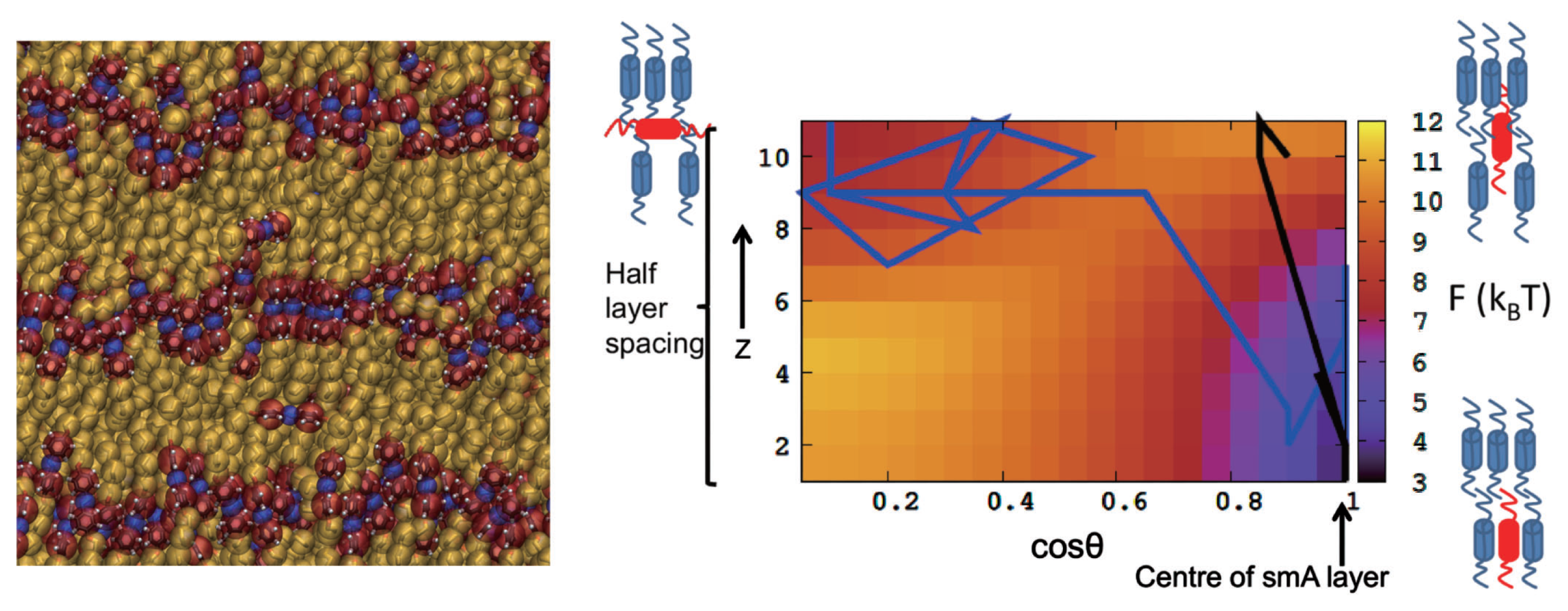
For an azobenzene-based liquid crystalline compound (8AB8) it was found that state point transferability could be achieved by choosing as an appropriate state point for the reference simulation the supercooled liquid just below the smectic-isotropic phase transition. This reference state is characterized by a high degree of local nematic order while being overall isotropic. The primary idea behind this choice of reference state is the observation that—in the spirit of arguments from classical density functional theories of liquids [157]—the short ranged correlations in the ordered phase are not very different from the local correlations present in a disordered phase at suitable thermodynamic state (density, temperature, etc.) (as one approaches the transition from the high-temperature side). If one captures these local correlations and builds them into the (structure-based) potentials, then these potentials should be able to describe phases on both sides of the transition. For 8AB8, indeed an excellent structural correspondence with the atomistic reference in the smectic state has been found. With the resulting CG model it is possible to switch between the atomistic and the CG levels (and vice versa) in a seamless manner maintaining values of all the relevant order parameters which describe the LC ordered state (see Figure 1). At the same time, this CG model shows remarkable state point transferability and reproduces the LC-isotropic phase transition upon heating and cooling [39]. Such a CG LC model—since it is on the one hand sufficiently coarse grained to study a variety of processes in the LC phase while being at the same time still very closely related to an underlying chemically realistic atomistic description, e.g., allowing for realistic molecular flexibility—is able to give new insights into for example microscopic dynamics in LC phases [40]

3. Adaptive Resolution Simulations

In the introduction we defined a class of systems for which the focus of the researcher’s interest is on a (possibly small) subregion of the simulated system: this is the case, for example, of the hydrogen bond network at the surface of a solvated molecule in water. The bulk of water molecules has to be simulated in order to sustain the thermodynamical properties of the subsystem of interest—the interfacial water—and to provide the correct exchange of molecules. Nonetheless, the fine-grained detail of molecules far from the interface is not relevant; it would be therefore desirable to replace the atomistic, expensive interactions of hydrogen and oxygen atoms with a coarser model.

We can then introduce a geometrical separation between an “inside” and an “outside”, i.e., an all-atom and a coarse-grained region, and assign different types of representations and interactions to the molecules according to their position in the simulation domain.

This idea has a long and successful history: to investigate crack propagation in hard matter, for example, several authors [158–162] made use of a hybrid description of the system, where a “high resolution” description is employed only for the area in the proximity of the crack, and the material far from the crack is treated with a simpler model. Another important example of hybrid resolution simulation is provided by Quantum Mechanics/Molecular Mechanics (QM/MM) methods [163–167]. In this case the structure of the system is described at the same (atomistic) level everywhere; however, the interactions are obtained from a classical force-field in the bulk of the system, but in a small region ab initio methods -such as Density Functional Theory, DFT- are employed to calculate the forces. Many different “flavors” of this approach have been developed; in all of them, though, one of the crucial aspects is how to interface the two domains where interactions are different, and in most of the established methods the identity or resolution of the particle is not allowed to change. In general, one has to answer the two following questions:

(1)

how should two atoms/molecules in different domains interact?

(2)

how should the properties of an atom/molecule change in crossing the interface?

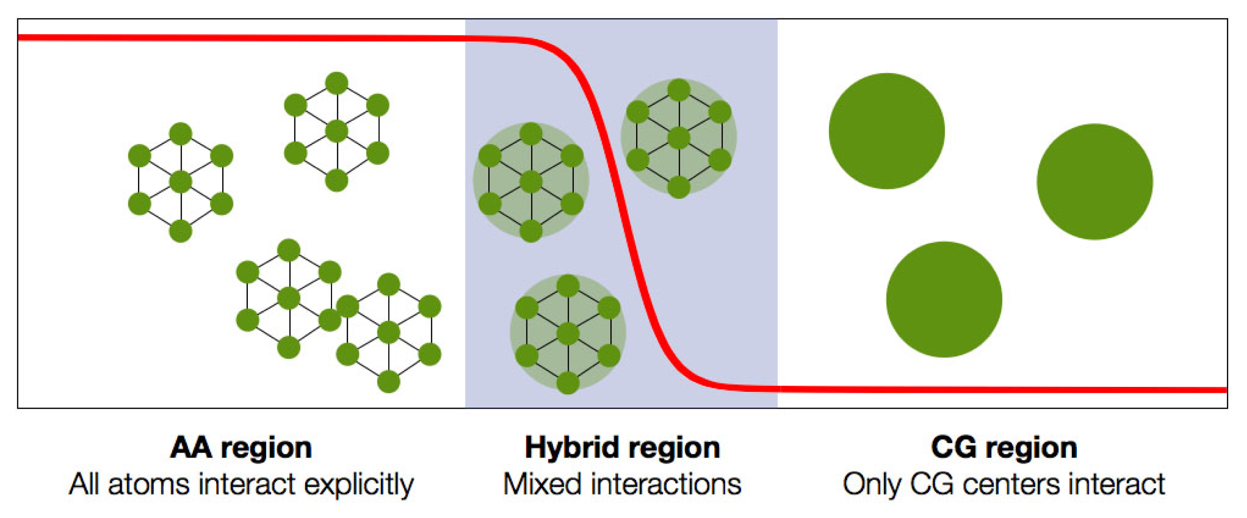
The last question is of particular importance for all systems whose components can diffuse on large length scales (at last of the order of the molecules’ size) in the simulation time. It appears natural to introduce a transition region (often called hybrid region, or healing region) that allows for a smooth interpolation from a given representation of the molecule’s structure/interaction to another; a schematic representation of this setup is provided in Figure 2. The choice of the specific way this interpolation is implemented depends, as we mentioned earlier, on the properties that have to be preserved in the CG region.

Irrespective of the chosen method to interface the two regions of the system, however, it is natural to expect that the equilibrium state that will be reached in the absence of external driving forces will not be the desired one. A further crucial point is then to find the simplest way to impose the desired thermodynamics.

The central, strong requirement that has to be satisfied is that molecules should be free to diffuse from any region of the simulation box to any other. Additionally, in a hybrid resolution model thermal equilibrium should be preserved, i.e., the temperature of the system has to be constant during the simulation. Another possible constraint is to impose a uniform density across the box, irrespective of the specific resolution; nonetheless, we’ll see that there are cases where this is neither strictly necessary nor desirable.

These are the fundamental constraints that can be imposed on the system as a whole. Other, more specific ones can be introduced on the properties of the CG region as well as the transition region, which will “drive” us towards a specific formulation of a double-resolution simulation method.

3.1. The Adaptive Resolution Simulation Scheme

The Adaptive Resolution Scheme (AdResS) represents the first effective and computationally efficient method to simulate a system where two different models, e.g., an all-atom one and a coarse-grained one, are simultaneously employed in different subregions of the simulation domain, interfaced in such a way to allow molecules to freely diffuse from one region to the other.

The basic constraint that was enforced in the original version of this scheme is that Newton’s 3rd law has to be exactly satisfied everywhere in the simulation domain. This requirement rules out any form of potential energy interpolation: it can in fact be formally demonstrated [168] that no method exists to smoothly “blend” the interaction between two molecules from a given potential energy to another without generating forces that cannot be recast in a form that satisfies Newton’s Third Law. In order to preserve the latter, then, a force-interpolation scheme is required, such that the force that a given molecule receives due to the interaction with a second one is antisymmetric under exchange of the molecules’ labels:

$${\mathbf{F}}_{\alpha \mid \beta }=-{\mathbf{F}}_{\beta \mid \alpha }$$

(20)

A second, less strict requirement is that CG molecules possess CG degrees of freedom only; this determines the specific way the force mixing is performed: a molecule in the CG region loses completely its atomistic detail (thus retaining, for example, the center of mass coordinates only), and interacts with a molecule in the AA or even the transition region only via its CG degrees of freedom. Formally, this constraint imposes that the atomistic forces vanish when at least one of the two interacting molecules is in the CG domain.

These two constraints are sufficient to define the force-field interpolation; the force acting between molecules α and β is given by:

$${\mathbf{F}}_{\alpha \beta }=\lambda ({\mathbf{R}}_{\alpha })\lambda ({\mathbf{R}}_{\beta }){\mathbf{F}}_{\alpha \beta }^{AA}+(1-\lambda ({\mathbf{R}}_{\alpha })\lambda ({\mathbf{R}}_{\beta }))\hspace{0.17em}{\mathbf{F}}_{\alpha \beta }^{CG}$$

(21)

In Equation (21) λ(x) is any smooth function that goes from 1 in the AA region to 0 in the CG region. R_α (resp. R_β) is the CoM coordinate of molecule α (resp. β). ${\mathbf{F}}_{\alpha \beta }^{AA}$ and ${\mathbf{F}}_{\alpha \beta }^{CG}$ are, respectively, the atomistic and the coarse-grained forces acting on molecule α due to the interaction with molecule β.

The CG force is computed between the coarse grained centers of the molecules and then redistributed to the atoms weighted by the ratio of the atom’s mass to the mass of molecule [169]; in the transition region this operation is required by the fact that molecules interact at both the AA and the CG level. AA degrees of freedom thus have to be explicitly integrated, at least into the hybrid region. In the CG region, on the other hand, it is in principle not necessary to conserve the atomistic detail of the molecules, so that the CG force could be applied directly to the CoM coordinate; a molecule’s internal structure can thus be removed when it enters the CG region, and reintroduced (e.g., taking it from a reservoir/repertoire of equilibrated atomistic molecules) as soon as it approaches the hybrid region. In all AdResS versions implemented so far, though, the atomistic DoFs are retained for simplicity of implementation [24]; the CoM of the molecule is nonetheless decoupled from the internal atomistic structure, and it evolves only subject to the CG force.

It was previously mentioned that no energy interpolation is possible, that is compatible with the requirement of having Newton’s 3rd law preserved everywhere in the system [168]; as a consequence, a force interpolation had to be chosen. It is evident, then, that the AdResS scheme cannot be formulated in terms of a Hamiltonian, thus making it impossible to perform microcanonical, i.e., energy-conserving simulations. The force-field used in this adaptive resolution simulation framework is not conservative in the transition region, and when crossing it a molecule receives a surplus of energy that has to be removed in order to prevent the system from artificially heating up. This excess energy can be removed with a local thermostat, such as Langevin thermostat: in this way, the temperature of the system is kept constant everywhere. The equilibrium state of the system is then dynamical: the thermostat takes care of absorbing the extra heat produced in the transition region by non-conservative forces, and the system samples equilibrium configurations according to Boltzmann’s distribution [24–32].

The pressure difference between an AA system and a low-resolution model typically resulting from coarse graining procedures determines the onset of a non-uniform density profile. For example, a one-site CG model of water obtained with IBI can have a pressure ~6000 times the atomistic reference value [117]. Therefore, the densities in the two subregions will change in order to equate the pressures. A possible solution to this density imbalance is to parametrize the CG potential to the target pressure. In the IBI framework this can be achieved by introducing a “pressure correction” [81]. This approach can provide a CG potential that has the target pressure, but this would also result in a modified compressibility [117].

Another option to preserve a uniform density across the simulation domain without modifying the CG potential is to introduce an external force which counterbalances the high pressure of the CG model. This thermodynamic force can be obtained with an iterative procedure via the following expression [169–171]:

$${\mathbf{f}}_{th}^{i+1}={\mathbf{f}}_{th}^i-\frac{1}{{\rho }^{★}{\kappa }_T}\nabla {\rho }^i(r)$$

(22)

where ρ^* is the reference molecular density, κ_T is the system’s isothermal compressibility and ρⁱ(r) is the molecular density profile as a function of the position in the direction perpendicular to the CG-AA interface. The thermodynamic force is initialized to zero, ${\mathbf{f}}_{th}^0=0$, while the initial density profile is the one calculated from an AdResS simulation with f_th = 0. As can be easily seen, the iterative procedure converges once the density profile is flat (∇ρ(r) = 0).

This approach guarantees a flat density profile without having to modify the CG potential: because of its very definition, the thermodynamic force only acts on those molecules that cross the hybrid region, leaving the others unaffected. It can also be shown [24,169] that the integral of the thermodynamic force across the interface, i.e., the work due to this force performed by a molecule while crossing the hybrid region, is proportional to the local pressure profile, the proportionality factor being the reference density ρ^*.

In summary, the thermodynamic force allows us to couple a system at atomistic resolution to a coarse-grained counterpart whose pressure, for given values of density and temperature, is significantly different. The global properties of the force, whose direct effect is restricted to the hybrid region, only depend on the pressure difference between the two coupled subsystems; the detailed profile of the force, on the other hand, can be obtained via a system-specific iterative procedure. This method not only allows one to preserve the desired structure of the system in the CG region; in principle, in fact, an arbitrary CG force-field, with pressure and structure completely different from the target atomistic ones, can be used. Consequently, the AA region behaves as an open system [169] that exchanges energy and molecules with a reservoir: the molecule number fluctuations, the pressure and all other thermodynamically relevant quantities are the same as if the AA region were simply ‘cut’ from a large all-atom simulations. It is relevant to stress here that because of the thermodynamic force this condition can be established irrespective of the specific model used in the CG region.

3.2. Applications

The possibility of treating a system with a reduced number of degrees of freedom except where it is strictly necessary was explored, making use of the AdResS method, in several applications [24–30,172]. From the numerical/computational point of view it clearly represents an advantage, since a much smaller number of force calculations are required in the coarse-grained region: this is particularly true for parallel MD codes such as GROMACS [173], where a dynamical decomposition of the simulation box allows one to subdivide the box with a finer grid in the AA and hybrid region, while a smaller number of processors is assigned to the CG region. For example, for a water system with an AA region covering 1/6 of the total simulation box, simulated with GROMACS on a 16-cores processor, the speed-up is about a factor three. This factor is nonetheless small compared to what can be achieved with other simulation packages, such as ESPRESSO++ [174]: in fact, water simulation in GROMACS is extremely optimized, and any hacking of the standard code can introduce a bottleneck.

A major strength of the AdResS method is the fact that it introduces a decoupling between a given region of the system and the rest while keeping the thermodynamic properties of both regions under control: as a consequence, it is possible to conceive numerical experiments in which the spatial extension of correlations in the system is investigated. More specifically, one can study the structural properties of the high-resolution region as a function of its size, in order to determine their dependency on the interaction with molecules in the bulk region. This kind of experiments is different from the study of finite-size effects: in the latter, in fact, the system has the same resolution and interaction type everywhere, and the change of a property with the box size depends on the asymptotic approach to the thermodynamic limit. In the AdResS setup, on the other hand, finite-size effect can be neglected for sufficiently large boxes, thus allowing one to characterize the response of the system’s properties in a small subregion when atomistic interactions with the bulk are switched off, but the thermodynamics is the same as in a fully-atomistic simulation. An example of this applications is provided by the work in Reference [175]: here a molecule with both hydrophilic and hydrophobic interactions was solvated in water and put at the center of the high-resolution region, while the water molecules far from the surface were treated at the coarse-grained level. The ordering degree of the hydrogen bond network on the molecule’s surface was measured as a function of the size of the all-atom region: the results showed a dependency of the ordering for water molecules close to the surface of the repulsive solute, while no relevant effect was observed for the attractive case.

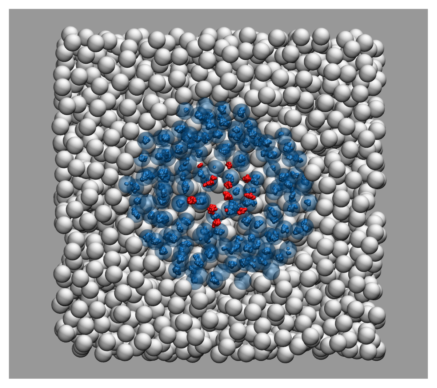
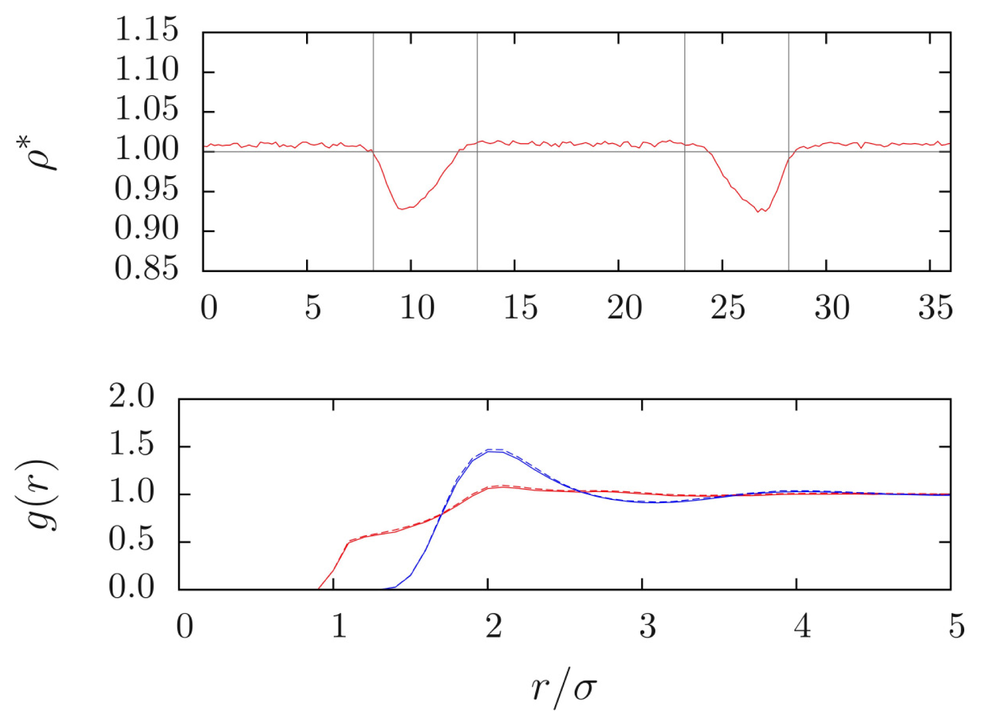
The same strategy has been applied to investigate the extent of spatial correlations in a quantum fluid, namely low-temperature para-hydrogen [30,176]. The latter is the spin-zero singlet state of molecular hydrogen. Because of the spherical symmetry of the global wave function, para-hydrogen in the solid and gas phase can be modeled as a classical, point-like particle interacting via a simple radial potential, such as Lennard-Jones or the more accurate Silvera-Goldman potential [177,178]. The same classical potential has been shown to correctly reproduce the experimental results both in the solid and the gas phase [178]. In the fluid phase, however, nuclear delocalization effects become important, and a quantum mechanical treatment of the problem is necessary. This can be achieved through the path integral formalism [179,180], which allows for the explicit inclusion of nuclear quantum effects in a “classical” description; unfortunately, this also implies a significant increase in the number of degrees of freedom that have to be simulated, since each molecule becomes a collection of P beads connected by springs. The possibility to simulate a quantum system in a classical framework such as classical MD makes it possible to couple quantum a classical descriptions with the AdResS scheme. In particular, a low-temperature para-hydrogen system was simulated making use of the explicit path integral representation only in a small spherical subregion of the domain, while the molecules in the outer region were treated at the purely classical level, i.e., point-like particles interacting through a coarse-grained potential [30]; in Figure 3 a snapshot of the simulated system is provided. This study showed that a few molecules in a small (~0.6 nm radius) region of the system are sufficient to reproduce the quantum pair correlation function obtained from a full path integral simulation, but treating the molecules in the outer region at the CG level; this result opens the way to simulate large systems of low-temperature para-hydrogen taking advantage of a double resolution without disrupting the thermodynamical and structural properties of the small, purely quantum region, thus saving computational time in the CG region.

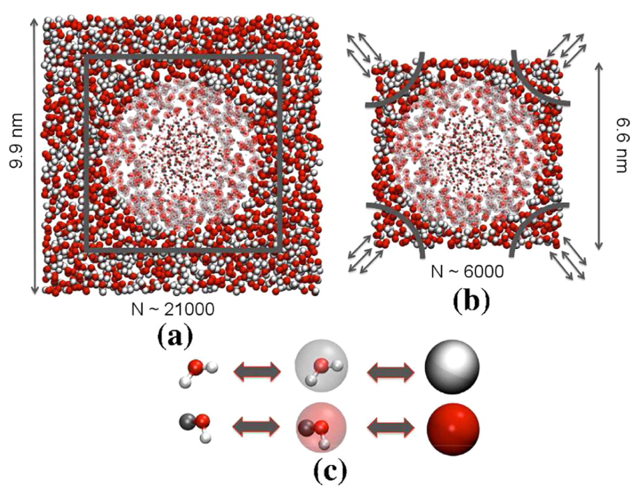
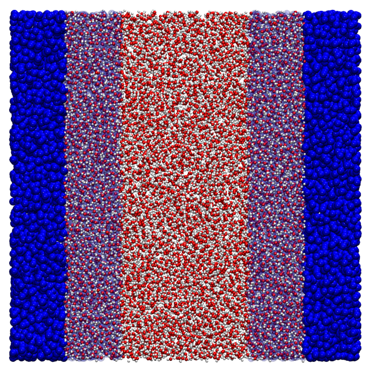
More recently the AdResS scheme has been successfully employed to perform simulations of biologically relevant systems such as methanol-water mixtures [181] and triglycine in aqueous urea [171], and to study the coil-globule transition of a PNIPAm molecule in aqueous methanol [182]. In all these cases a crucial necessity is to correctly reproduce the solvation free energies of the system, a condition that is verified only when the particle number fluctuations are compatible with those observed in the Grand Canonical ensemble. The large system sizes necessary to fulfill this requirement in a standard, all atom simulation often make the latter unfeasible; the employment of dual-resolution simulation methods, possibly coupled to a Monte Carlo scheme [182] to enforce fluctuations in the total number of molecules, see Figure 4, allows one to keep the computational cost low and obtain results that would otherwise require a significantly longer time.

3.3. The Limitations of the Force-Based Approach

The AdResS method discussed so far represents a simple, effective way to perform double-resolution simulations, i.e., simulations where the model used to represent a molecule and its interactions with the others changes according to the molecule position. Assigning the lowest-resolution model to the largest region allows one to save computational resources and characterize the bulk dependence of structural properties of the high-resolution subsystem. A majorly important point is given by the possibility to keep the thermodynamics of the system under control: this can be achieved by direct intervention on the CG model’s properties, or by introducing an external field -the thermodynamic force- in the hybrid region to compensate for density imbalances. This second streategy is crucial, since it allows one to couple arbitrarily different systems while keeping locally well-defined temperature, pressure and energy.

The AdResS method was conceived based on the requirement that Newton’s Third Law has to be exactly satisfied everywhere. This constraint poses a strict limitation to the possible ways to interface the two representations of the system: specifically, no potential energy interpolation is possible, via a position-dependent switching function, that preserves Newton’s Third Law [168]; as a consequence, the only acceptable interpolation can be performed on the forces.

A posteriori, the lack of a global energy function proves not to be a major problem: equilibrium and canonical sampling can be enforced making use of a local Langevin thermostat. A theoretical analysis of the AdResS dual resolution scheme has been recently carried out in Reference [183], where the presence of a local thermostat and the thermodynamic force have been shown to be necessary and sufficient conditions to guarantee the equivalence of the atomistic region to an open region of a fully atomistic simulation up to second order correlation functions (density profile and radial distribution function). These results have been obtained from a completely general model of a dual resolution setup under the assumption of the thermodynamic limit; the generality of this approach makes it thus applicable to different types of adaptive resolution schemes, independently of the detailed form of the method chosen to interpolate the resolutions.

Nonetheless, the lack of a Hamiltonian has negative consequences on the usage of the AdResS method; the four major ones are: microcanonical, i.e., energy-conserving simulation are not possible; no partition function can be written for the system as a whole; no Monte Carlo scheme can be implemented. Finally, due to the non-conservative nature of the forces in the hybrid region the system necessarily has to be locally thermostatted to compensate for the heat that is produced in the hybrid region, so that an AdResS simulation is found to be in a state of dynamical equilibrium [32], with a constant flux of heat between the system and the thermostat.

In the next section a method is discussed, named H-AdResS [33] (for Hamiltonian Adaptive Resolution Simulation scheme), that provides a solution to the aforementioned problems; clearly, as no free lunch is usually available, there is a price to pay: the Hamiltonian formulation requires a local breakdown of Newton’s Third Law.

3.4. The Hamiltonian Adaptive Resolution Scheme

As was discussed in the previous section, the force-based AdResS method was developed on the basis of a central requirement, namely that Newton’s 3rd law has to be exactly satisfied everywhere. A consequence of this constraint is that no Hamiltonian formulation is possible [168]: if a position-dependent interpolation of the potential energies is done, in fact, the resulting forces include a term proportional to the derivatives of the switching function λ that cannot be recast in a form that satisfies Newton’s Third Law. The only method developed in the past that allows one to explicitly conserve the energy in an adaptive resolution simulation is that proposed by Heyden and Truhlar, [184,185], where a sum of the Lagrangians of all possible groupings of atomistic and coarse-grained molecules is done. Due to its combinatoric nature, this approach is extremely difficult to implement efficiently; moreover, the resulting Lagrangian includes a position-dependent kinetic energy term for which a specific, non-symplectic integrator is required.

In the H-AdResS method [33], which we now describe, the aforementioned constraints are relaxed in order to develop an energy-based, Hamiltonian adaptive resolution simulation scheme. As will be clear in a few lines, the particular choice of energy “mixing” gives rise to forces that do not comply with the first constraint; nevertheless, the physical interpretation of these terms is immediate and naturally points towards the solution -though approximate- of the Newton’s Third Law breakdown.

The core idea of the energy-based approach is to weight the total energy of each molecule with a position-dependent function:

$$H=\mathcal{K}+V^{int}+\sum _{\alpha }\{{\lambda }_{\alpha }{V}_{\alpha }^{AA}+(1-{\lambda }_{\alpha })V_{\alpha }^{CG}\}$$

(23)

where is the (all-atom) kinetic energy of the molecules, V^int is the interaction internal to the molecules, and:

$$\{\begin{array}{l}{V}_{\alpha }^{AA}\equiv \frac{1}{2}\sum _{\beta ,\beta \ne \alpha }^N\sum _{ij}{V}^{AA}(\mid {\mathbf{r}}_{\alpha i}-{\mathbf{r}}_{\beta j}\mid )\\ V_{\alpha }^{CG}\equiv \frac{1}{2}\sum _{\beta ,\beta \ne \alpha }^N{V}^{CG}(\mid {\mathbf{R}}_{\alpha }-{\mathbf{R}}_{\beta }\mid )\\ {\lambda }_{\alpha }=\lambda ({\mathbf{R}}_{\alpha })\end{array}$$

The switching function λ goes from 0 (purely CG) to 1 (purely AA). The force acting on atom i in molecule α is obtained through differentiation of the Hamiltonian in Equation (23):

$${\mathbf{F}}_{\alpha i}={\mathbf{F}}_{\alpha i}^{int}+\sum _{\beta ,\beta \ne \alpha }\left\{\frac{{\lambda }_{\alpha }+{\lambda }_{\beta }}{2}{\mathbf{F}}_{\alpha i\mid \beta }^{AA}+\left(1-\frac{{\lambda }_{\alpha }+{\lambda }_{\beta }}{2}\right)\hspace{0.17em}{\mathbf{F}}_{\alpha i\mid \beta }^{CG}\right\}-[V_{\alpha }^{AA}-V_{\alpha }^{CG}]{\nabla }_{\alpha i}{\lambda }_{\alpha }$$

(24)

The forces ${\mathbf{F}}_{\alpha i\mid \beta }^{AA}$ and ${\mathbf{F}}_{\alpha i\mid \beta }^{CG}$ are defined as:

$$\begin{array}{l}{\mathbf{F}}_{\alpha i\mid \beta }^{AA}\equiv \sum _{j=1}^{n_{\beta }}-\frac{\partial }{\partial {\mathbf{r}}_{\alpha i}}V(\mid {\mathbf{r}}_{\alpha i}-{\mathbf{r}}_{\beta j}\mid )\\ {\mathbf{F}}_{\alpha i\mid \beta }^{CG}\equiv -\frac{m_{\alpha i}}{M_{\alpha }}\frac{\partial }{\partial {\mathbf{R}}_{\alpha }}{V}^{CG}(\mid {\mathbf{R}}_{\alpha }-{\mathbf{R}}_{\beta }\mid )\end{array}$$

(25)

The redistribution of the CG force on the atomistic degrees of freedom follows the same rules as applied in the case of the force-based AdResS method. It’s worth noting that in this energy-based scheme the atomistic degrees of freedom are retained and integrated everywhere in the system, a necessary requirement in order to perform a microcanonical simulation making use of a Hamiltonian.

We now detail the various components of the force, Equation (24). The first term, ${\mathbf{F}}_{\alpha i}^{int}$ is due to the interactions internal to the molecule; as such, it automatically satisfies Newton’s Third Law. The second term is a sum of pairwise forces obtained from all-atom and coarse-grained Hamiltonians, weighted by a function that is symmetric under molecule label exchange, that is α ↔ β; this force also complies with Newton’s Law. Up to this point we modified only one aspect of the original AdResS scheme, that is, the force weights are not given by the product of the two molecules’ switching function, rather by the average; consequently, the molecules in the coarse-grained region are also allowed to interact through their atomistic degrees of freedom.

The third term of the forces in Equation (24) is the part that breaks down Newton’s Third Law: in fact, it cannot be written as a sum of terms antisymmetric under molecule label exchange. This force, which is nonzero only in the hybrid region, is proportional to the difference between the potential energies of a given molecule in the AA and the CG representation; if a systematic difference exists between the AA and the CG potentials, the effect of this term is to push molecules into one of the two bulk regions. The hybrid region thus behaves as an active membrane, inducing a density imbalance and a non-flat pressure profile. One is then naturally led to ask how strong is the drift term ${\mathbf{F}}_{\alpha }^{dr}=-[V_{\alpha }^{AA}-V_{\alpha }^{CG}]{\nabla }_{\alpha i}{\lambda }_{\alpha }$; if it is negligible in some cases; which these cases are; and if there is a general way at least to minimize its effect without giving up the Hamiltonian character of these forces. We shall now address these questions.

The optimal case in which this term is minimized is when the CG potential perfectly reproduces the many-body PMF. If this is true, in fact, the drift term vanishes on average:

$$V_{\alpha \beta }^{CG}\equiv \langle V_{\alpha \beta }^{AA}\rangle \Rightarrow \langle {\mathbf{F}}_{\alpha }^{dr}\rangle \propto \langle [V_{\alpha }^{AA}-V_{\alpha }^{CG}]\rangle \to 0$$

This can be numerically verified with a simple toy model, for which a pairwise CG potential represents an excellent approximation to the PMF. Such a model is provided by a low-density fluid of purely repulsive tetrahedral molecules [24], whose CG potential has been obtained from IBI. This model was used in an energy-conserving H-AdResS simulation, and the resulting density profile is plotted in Figure 5. The molecular density attains the same value in both the AA and CG regions; in the hybrid region a small depletion is present, because the free energy of the mixed potential is different from the free energy of the “pure” (i.e., purely AA or purely CG) potentials. The same behavior has been systematically observed in AdResS simulations [24].

Needless to say, this particular case is very fortunate: as we discussed in the previous sections, the CG potentials almost never reproduce the many-body potential of mean force [117,186]. The difference between an atomistic model and its coarse-grained representation therefore results in a thermodynamic imbalance, that is, both pressure and density of the two bulk (AA and CG) regions are different [13]. The solution to this problem is again to introduce a compensation term in the Hamiltonian, as was done in the AdResS scheme with the thermodynamic force. More specifically, we modify the Hamiltonian as follows:

$$H_{\mathrm{\Delta }}=H-\sum _{\alpha =1}^N\mathrm{\Delta }H(\lambda ({\mathbf{R}}_{\alpha }))$$

(26)

where ΔH(λ) is a function to be defined. It’s worth noting that this term preserves the conservative nature of the Hamiltonian.

In order to determine the specific form of ΔH we impose that the drift force cancels on average:

$${\frac{d\mathrm{\Delta }H(\lambda )}{d\lambda }|}_{{\lambda }_{\alpha }}{\nabla }_{\alpha }{\lambda }_{\alpha }+\langle {\mathbf{F}}_{\alpha }^{dr}\rangle \equiv 0$$

(27)

or equivalently:

$${\frac{d\mathrm{\Delta }H(\lambda )}{d\lambda }|}_{\lambda ={\lambda }_{\alpha }}={\langle [V_{\alpha }^{AA}-V_{\alpha }^{CG}]\rangle }_{{\mathbf{R}}_{\alpha }}$$

(28)

where the subscript in the average indicates that the latter has to be performed constraining the CG site of molecule α in the position R_α.

In principle, Equation (28) provides us with the way to compute the compensating function—or, more precisely, its derivative; nonetheless, an approximation to ΔH might be sufficient. A way to do this is the following:

$${\langle [V_{\alpha }^{AA}-V_{\alpha }^{CG}]\rangle }_{{\mathbf{R}}_{\alpha }}\simeq \frac{1}{N}{\langle [V^{AA}-V^{CG}]\rangle }_{{\lambda }^{\prime }}$$

(29)

where λ′ ≡ λ(R_α) is the same for all molecules. The approximate function ΔH is obtained by integration:

$$\mathrm{\Delta }H(\lambda )={\int }_0^{\lambda }d{\lambda }^{\prime }\frac{d\mathrm{\Delta }H({\lambda }^{\prime })}{d{\lambda }^{\prime }}\simeq \frac{1}{N}{\int }_0^{\lambda }d{\lambda }^{\prime }{\langle [V^{AA}-V^{CG}]\rangle }_{{\lambda }^{\prime }}=\frac{\mathrm{\Delta }F(\lambda )}{N}$$

Most interestingly, we see from Equation (30) that the compensation needed to cancel $\langle {\mathbf{F}}_{\alpha }^{dr}\rangle$ is related to the Helmholtz free energy difference between AA and CG system [187]. Therefore, it is possible to calculate the compensating function needed to restore, on average, Newton’s Third Law by performing a Kirkwood thermodynamic integration.

The “Helmholtz free energy compensation” thus cancels the active effect of the hybrid region, restoring a flat pressure profile. Nonetheless, coarse-grained models have, in general, a substantially different pressure with respect to their atomistic reference [117], thus inducing a further density imbalance (usually larger than the one due to the different Helmholtz free energy). In order to restore a flat density profile a second term has then to be added to the compensating function, that counterbalances the pressure difference.

The right way to introduce the pressure into the compensating function is to balance, rather than Helmholtz free energy, the Gibbs free energy difference per particle, that is, the chemical potential Δμ = ΔG/N:

$$\mathrm{\Delta }H(\lambda )\equiv \mathrm{\Delta }\mu (\lambda )=\frac{\mathrm{\Delta }F(\lambda )}{N}+\frac{\mathrm{\Delta }p(\lambda )}{{\rho }^{★}}$$

(30)

Figure 6 shows the density and pressure profiles for the three possible cases we discussed: the previously mentioned system of tetrahedral molecules was coupled to a coarse-grained fluid of purely repulsive point-like molecules; the pressure of this fluid has a larger pressure then the reference all-atom one for the same temperature and density. In the plot, the red lines correspond to the case in which no free energy compensation is introduced: the density is higher in the AA region, due to the molecules in the CG region that “push” with a higher pressure. The profile of the pressure is also not flat: the Helmholtz free energy of two systems differs, therefore an active force exists in the hybrid region. When the Helmholtz free energy compensation is applied we have the situation shown by the green lines: the density is still higher in the AA region, but the pressure profile is now flat: the forces that break Newton’s Third Law in the hybrid region are cancelled on average, and the density imbalance decreases. Finally, when the Gibbs free energy compensation is applied the densities of the AA and CG regions attain the same value, but for a small deviation due to the fluctuations present in the hybrid region (that the compensation function ΔH, computed in a homogeneous system, cannot remove). The pressure, on the other hand, is different: in fact, in each region it reaches the value that corresponds to the reference state of density and temperature. Analogous results are obtained in a thermostatted simulation of a water box, as shown in Figure 7: here the system is composed of a slab of water molecules described at atomistic resolution, coupled to a CG bulk where particles interact via a purely repulsive WCA potential. As in the previous case, the CG interaction was parametrized to induce an increase of the density in the atomistic region, as can be seen in Figure 8 (upper panel). The Free Energy Compensation restores the correct density profile, and guarantees that in the AA region the pairwise correlations, i.e., the radial distribution functions, are the same that one would measure in a fully atomistic simulation, as shown in Figure 8 (bottom panel). We notice that Gibbs free energy compensation, even though it equates the densities in the bulk regions, is not sufficient to remove small fluctuations (of the order of ~3%) in the hybrid region: these deviations from the reference value are due to the fact that the compensation ΔH is computed in a homogeneous system, where all molecules have the same value of λ—that is, a regular Kirkwood thermodynamic integration Hamiltonian. The molecules in the hybrid region, on the other hand, interact with other molecules having different λ values. The resulting fluctuations are expected to decrease with increasing size of the hybrid region, in which case the environment of a given molecule approaches the condition of homogeneous λ. Another strategy to flatten the density profile is clearly provided by the iterative approach of the thermodynamic force (Equation (22)), a few iterations of which would be sufficient to modify the ΔH function by the small amount necessary to remove the fluctuations.

The Free Energy Compensation (FEC) strategy, defined by Equation (26), can be extended to multi-component systems. To illustrate this idea we consider a molecular liquid composed by two types of molecules, A and B, indexed with a and b, respectively. The corresponding H-AdResS Hamiltonian for this system reads:

$$H^{MIX}=K+V^{int}+\sum _{a\in A}[{\lambda }_a{V}_a^{AA}+(1-{\lambda }_a)V_a^{CG}]+\sum _{b\in B}[{\lambda }_b{V}_b^{AA}+(1-{\lambda }_b)V_b^{CG}]$$

(31)

with λ_a = λ(R_a) and λ_b = λ(R_b). The intermolecular potential energy terms are given by the following expressions:

$$\begin{array}{l}{V}_a^{AA}=\frac{1}{2}\hspace{0.17em}\left[\sum _{\begin{array}{l}{a}^{\prime }\in A\\ a^{\prime }\ne a\end{array}}\sum _{ij}V{[AA]}_{ai;a^{\prime }j}^{AA}+\sum _{b\in B}\sum _{ij}V{[AB]}_{ai;bj}^{AA}\right]\\ V_a^{CG}=\frac{1}{2}\hspace{0.17em}\left[\sum _{\begin{array}{l}{a}^{\prime }\in A\\ a^{\prime }\ne a\end{array}}V{[AA]}_{a{a}^{\prime }}^{CG}+\sum _{b\in B}V{[AB]}_{ab}^{CG}\right]\\ V_b^{AA}=\frac{1}{2}\hspace{0.17em}\left[\sum _{\begin{array}{l}{b}^{\prime }\in B\\ b^{\prime }\ne b\end{array}}\sum _{ij}V{[BB]}_{bi;b^{\prime }j}^{AA}+\sum _{a\in A}\sum _{ij}V{[AB]}_{bi;aj}^{AA}\right]\\ V_b^{CG}=\frac{1}{2}\left[\sum _{\begin{array}{l}{b}^{\prime }\in B\\ b^{\prime }\ne b\end{array}}V{[BB]}_{b{b}^{\prime }}^{CG}+\sum _{a\in A}V{[AB]}_{ba}^{CG}\right]\end{array}$$

(32)

where V [XY ] is the non-bonded interaction between a molecule of type X and a molecule of type Y, with X, Y = A, B, and the indices i, j labeling the atoms.

In analogy with one-component systems we introduce a FEC term for each species to compensate for the free energy difference between the AA and the CG regions:

$$H_{\mathrm{\Delta }}^{MIX}=H^{MIX}-\sum _{a\in A}\mathrm{\Delta }{H}_A({\lambda }_a)-\sum _{b\in B}\mathrm{\Delta }{H}_B({\lambda }_b)$$

(33)

An Ansatz for the compensation term of a given species k = a, b can be obtained from TI as follows:

$$\begin{array}{l}\mathrm{\Delta }{H}_k(\lambda )=\frac{\mathrm{\Delta }{F}_k(\lambda )}{N_k}+\frac{\mathrm{\Delta }{p}_k(\lambda )}{{\rho }_k^{★}}\\ \mathrm{\Delta }{F}_k(\lambda )={\int }_0^{\lambda }d{\lambda }^{\prime }{\langle [V_k^{AA}-V_k^{CG}]\rangle }_{{\lambda }^{\prime }}\\ \mathrm{\Delta }{p}_k(\lambda )=p_k(\lambda )-p_k(0)\end{array}$$

(34)

where the N_k, ${\rho }_k^{★}\equiv N_k/V$ and p_k are, respectively, the number of molecules, the reference partial density and the partial virial pressure of species k. We stress that all the quantities in Equation (34) can be computed in a single TI of the mixture from AA to CG at the concentration of interest, irrespective of the number of species. All the cross-interactions between different types of molecules are automatically included in the free energy contribution of each species. Additionally, the Free Energy Compensation ΔH_k(λ) is an intensive quantity and does not depend on the specific geometry of the H-AdResS setup. It is therefore possible to perform the TI in a relatively small system, provided that it is statistically representative, i.e., finite size effects are negligible.

The effectiveness of this strategy has been proven by the Monte Carlo simulations of binary mixtures performed in Reference [34]. Here we report one of these simulations, specifically the mixture of 70% A-type molecules and 30% B-type molecules, both made of four identical atoms; the A–A and B–B interactions are identical WCA potentials, while the A–B interaction is a Lennard-Jones potential. In the CG region both molecules are represented as spherical particles with identical, purely repulsive WCA A–A, B–B and A–B interactions, resulting in a particularly large thermodynamic mismatch between AA and CG domains. This can be directly observed in the snapshot of the simulation reported in Figure 9 (top) as well as in the density profiles (dotted lines in Figure 10): the chemical potential imbalance between the two resolutions leads to a large accumulation of B-molecules in the AA zone. As a consequence, neither the total density nor the relative concentrations in the AA zone obtained using the uncompensated adaptive resolution Hamiltonian in Equation (31) correspond to the reference atomistic system.

According to Equation (34), a thermodynamic integration was performed to determine the thermodynamic mismatch between the AA and the CG zone. The Helmholtz and Gibbs free energy differences per molecule between the CG and AA models as a function of the coupling parameter λ, computed for both species simultaneously in a single TI, are shown in Figure 11. In spite of the same interaction between molecules of the same type (V [AA] ≡ V [BB]), the uneven relative concentration of the two species determines a much larger free energy difference between the AA and CG models for the B-type. In fact, the latter shows a Gibbs free energy difference per particle |ΔG_B/N_B|> 2 |ΔG_A/N_A|. This is mainly due to the fact that the interaction between A and B types is attractive only in the AA representation, thus determining a lower chemical potential for the minority type (B) in the AA region. In addition, in both cases the sign of ΔG favors the densification of particles in the AA region, as can be seen in Figure 10. To counterbalance the mismatch in chemical potentials a FEC was introduced in the H-AdResS Hamiltonian according to Equation (33), using the free energy functions shown in Figure 11. The resulting density profiles (solid lines in Figure 10) demonstrate the success of the procedure.

In this section we discussed the H-AdResS method, which allows for a seamless coupling of two models of the same system with different resolution within a Hamiltonian framework. In order to define an energy-based mixing rule for the two models, the requirement to preserve Newton’s Third Law everywhere in the system had to be relaxed. Nonetheless, the “undesired” term that appears in the forces due to the differentiation of the switching function λ is non-zero only in the hybrid region, and its particular form naturally indicates how to introduce, in a physically sound manner, a compensation function that cancels the average effect of the drift force without disrupting the Hamiltonian character of the model. The computational cost of the H-AdResS simulations is comparable to that of the AdResS method, the only difference being the need to calculate the drift force ${\mathbf{F}}_{\alpha }^{dr}$ in the hybrid region: nonetheless, the number of molecules that are affected by this force is typically small (both the AA and the CG regions are expected to be much larger than the hybrid region), and the quantities involved, namely interaction energies and molecules’ CoM coordinates, are normally computed in a MD simulation.

In spite of its simple formulation and relatively small difference with respect to the force-based method, H-AdResS represents a major step forward in terms of understanding and practical advantages. In fact, the existence of a Hamiltonian allows one to precisely formulate a statistical physics theory of double-resolution systems, providing a deep insight into the properties of a given all-atom model, its coarse-grained counterpart and the relation between them. In particular, the free energy compensations provide a simple and effective way to modulate the thermodynamic balance of AA and CG regions, thus leaving to the user the choice of the environment for the AA region most appropriate for the specific problem under examination. Last but not least, this scheme broadens the spectrum of physical ensembles that can be simulated to the microcanonical ensemble, and allows the use use of simulations techniques—e.g., Monte Carlo—that were not accessible in the force-based AdResS framework, with the a priori guarantee that real equilibrium configurations are sampled.

4. Conclusions

The characterization of the properties of new materials, as well as the investigation of biological macromolecular machineries, have largely benefited from in silico experiments. In spite of a steady increase in available computational power for very large systems and long timescales of the processes involved these resources turn out to be insufficient, due to the extraordinarily large amount of data that has to be stored and force/energy calculations that have to be performed. To overcome these limitations, the field of multiscale simulations has vastly expanded over recent years, and in the present review we have covered two aspects that are central to many multiscale approaches.

In the first part of the review we have addressed methodological questions associated with the development of coarse grained models, where atoms are grouped into super-atoms to reduce the number of degrees of freedom in the system. We have summarized the current approaches to bottom-up coarse graining and addressed some of the ongoing coarse graining issues such as the choice of parametrization targets and the choice of interaction functions used for the coarse grained model. These choices lead to several possibilities (i.e., coarse graining methodologies) for solving the inverse problem of finding parameters for the coarse grained interaction functions given the selected target properties. We have briefly discussed these (statistical-mechanically interrelated) methods in context with each other. An inevitable question that arises from having to choose coarse graining target properties and approximations to solve the parametrization problem is the question of representability of different thermodynamic and structural properties. These representability challenges go hand in hand with the question of transferability, i.e., to which extent a reduced-resolution model is applicable to a state-point that is different from the one where it was parametrized. In general it can be said that transferability problems increase with decreasing level of resolution, i.e., the coarser a model the more limited is its applicability range, which then needs to be very carefully assessed. However, as a positive aspect one should mention that the investigation of transferability issues can help to gain insight into physical-chemical principles that drive the behavior of the system. We have illustrated transferability-related questions with the help of a few examples. In conclusion, one should mention that transferability problems are not specific to coarse grained models. Such problems are well known for classical atomistic forcefield models as well. A good example is simulations of mineral systems in contact with electrolyte or polyelectrolyte solutions. Here, forcefields for ions in solution and in the mineral solid have to be combined. This combination leads to transferability issues since electronic polarizability is not represented in a classical atomistic forcefield, and the compromises that are made to approximately account for its effects in a classical parametrization are different in the different phases. As a consequence, the typical “recipes” to combine parameters for different components cannot be straightforwardly applied, resulting in a significant parametrization effort for such problems [188–190]. The increasing awareness of transferability as a modeling challenge and the solution strategies developed in the context of coarse grained models may therefore very well benefit other areas of model development such as classical atomistic force-fieds for multicomponent materials systems.

In the second part of the review we have discussed the recent advances in the field of adaptive resolution approaches. The above mentioned limitation in system size comes together with the disappointing fact that a considerable fraction of the simulated data is often discarded afterwards: the solvent, for example, is usually not involved in the analysis of the system, but it is nonetheless required by the simulation. Adaptive resolution methods try to reduce the amount of resources dedicated to the simulation of large, non-interesting regions of the system by replacing them with a simpler, coarse-grained representation of their content. Such “dual-resolution” schemes are built with the constraint that the thermodynamical properties of the region of interest (i.e., the one with the higher resolution) do not differ from those that an equivalent subdomain of the system would have in a fully high-resolution simulation.

In the present work we discussed two methods to achieve this goal: the Adaptive Resolution Simulation (AdResS) scheme, based on the interpolation of two different force-fields, and its Hamiltonian formulation, H-AdResS, where the all-atom and coarse-grained potential energies are interpolated. These methods have been successfully used to interface different molecular fluids, treated at the atomistic level, with their coarse-grained models; the different properties of the AA and the CG potentials naturally induce thermodynamical imbalances in the corresponding sub-regions, but simple and effective ways to overcome this problem have been described.

The possibility of replacing vast regions of the simulated system with a crude, cheap-to-compute representation and concentrating the computational resources on smaller parts while keeping the relative thermodynamics under control makes it possible to sensibly reduce the amount of calculations required to perform a simulation, and opens the way to a broad spectrum of applications, such as large-scale simulations of complex biomolecules in solution and efficient open-boundary simulations with varying number of particles.

References

- Alder, B.; Wainwright, T. Phase transition for a hard sphere system. J. Chem. Phys 1957, 5, 1208–1209. [Google Scholar]
- Grest, G.; Kremer, K. Molecular dynamics simulation for polymers in the presence of a heat bath. Phys. Rev. A 1986, 33, 3628–3631. [Google Scholar]
- Kremer, K.; Grest, G.; Carmesin, I. Crossover from Rouse to Reptation Dynamics: A Molecular-Dynamics Simulation. Phys. Rev. Lett 1988, 61, 566–569. [Google Scholar]
- McCammon, J.; Karplus, M. Internal motions of antibody molecules. Nature 1977, 268, 765–766. [Google Scholar]
- Karplus, M.; McCammon, J. Protein structural fluctuations during a period of 100 ps. Nature 1979, 277, 578–578. [Google Scholar]
- Raiteri, P.; Laio, A.; Gervasio, F.L.; Micheletti, C.; Parrinello, M. Efficient reconstruction of complex free energy landscapes by multiple walkers metadynamics. J. Phys. Chem. B 2006, 110, 3533–3539. [Google Scholar]
- Lou, H.; Cukier, R.I. Molecular dynamics of apo-adenylate kinase: A distance replica exchange method for the free energy of conformational fluctuations. J. Phys. Chem. B 2006, 110, 12796–12808. [Google Scholar]
- Arora, K.; Brooks, C.L. Large-scale allosteric conformational transitions of adenylate kinase appear to involve a population-shift mechanism. Proc. Natl. Acad. Sci. USA 2007, 104, 18496–18501. [Google Scholar]
- Pontiggia, F.; Zen, A.; Micheletti, C. Small and large scale conformational changes of adenylate kinase: a molecular dynamics study of the subdomain motion and mechanics. Biophys. J 2008, 95, 5901–5912. [Google Scholar]
- Kremer, K. Computer simulations in soft matter science. In Soft and Fragile Matter: Non Equilibrium Dynamics, Metastability And Flow; IOP Publishing Ltd: Bristol, UK, 2000; SUSSP Proceedings, Volume 53; pp. 145–184. [Google Scholar]
- Kremer, K.; Müuller-Plathe, F. Multiscale problems in polymer science: Simulation approaches. MRS Bull 2001, 26, 205–210. [Google Scholar]
- Van der Vegt, N.A.; Peter, C.; Kremer, K. Structure-Based Coarse- and Fine-Graining in Soft Matter Simulations; CRC Press—Taylor and Francis Group: Boca Raton, FL, USA, 2009; pp. 379–397. [Google Scholar]
- Hijón, C.; Vanden-Eijnden, E.; Delgado-Buscalioni, R.; Español, P. Mori-Zwanzig formalism as a practical computational tool. Faraday Discuss 2010, 144, 301–322. [Google Scholar]
- Noid, W. Systematic Methods for Structurally Consistent Coarse-Grained Models. In Biomolecular Simulations; Humana Press: New York, NY, USA, 2013; Volume 924, pp. 487–531. [Google Scholar]
- Noid, W.G. Perspective: Coarse-grained models for biomolecular systems. J. Chem. Phys 2013, 139, 090901. [Google Scholar]
- Yelash, L.; Mueller, M.; Paul, W.; Binder, K. How well can coarse-grained models of real polymers describe their structure? The case of polybutadiene. J. Chem. Theory Comput 2006, 2, 588–597. [Google Scholar]
- Spyriouni, T.; Tzoumanekas, C.; Theodorou, D.; Müller-Plathe, F.; Milano, G. Coarse-Grained and Reverse-Mapped United-Atom Simulations of Long-Chain Atactic Polystyrene Melts: Structure, Thermodynamic Properties, Chain Conformation, and Entanglements. Macromolecules 2007, 40, 3876–3885. [Google Scholar]
- Tirion, M.M.; ben Avraham, D. Normal mode analysis of G-actin. JMB 1993, 230, 186–195. [Google Scholar]
- Tirion, M.M. Large amplitude elastic motions in proteins from a single–parameter, atomic analysis. Phys. Rev. Lett 1996, 77, 1905–1908. [Google Scholar]
- Bahar, I.; Atilgan, A.R.; Erman, B. Direct evaluation of thermal fluctuations in proteins using a single parameter harmonic potential. Fold. Des 1997, 2, 173–181. [Google Scholar]
- Micheletti, C.; Carloni, P.; Maritan, A. Accurate and efficient description of protein vibrational dynamics: comparing molecular dynamics and Gaussian models. Proteins 2004, 55, 635–645. [Google Scholar]
- Potestio, R.; Pontiggia, F.; Micheletti, C. Coarse-grained description of proteins’ internal dynamics: An optimal strategy for decomposing proteins in rigid subunits. Biophys. J 2009, 96, 4993–5002. [Google Scholar]
- Globisch, C.; Krishnamani, V.; Deserno, M.; Peter, C. Optimization of an Elastic Network Augmented Coarse Grained Model to Study CCMV Capsid Deformation. PLoS One 2013, 8, e60582. [Google Scholar]
- Praprotnik, M.; Delle Site, L.; Kremer, K. Adaptive resolution molecular-dynamics simulation: Changing the degrees of freedom on the fly. J. Chem. Phys 2005, 123, 224106–224114. [Google Scholar]
- Praprotnik, M.; Delle Site, L.; Kremer, K. Adaptive resolution scheme for efficient hybrid atomistic-mesoscale molecular dynamics simulations of dense liquids. Phys. Rev. E 2006, 73, 066701. [Google Scholar]
- Praprotnik, M.; Delle Site, L.; Kremer, K. A macromolecule in a solvent: Adaptive resolution molecular dynamics simulation. J. Chem. Phys 2007, 126, 134902. [Google Scholar]
- Praprotnik, M.; Delle Site, L.; Kremer, K. Multiscale Simulation of Soft Matter: From Scale Bridging to Adaptive Resolution. Ann. Rev. Phys. Chem 2008, 59, 545–571. [Google Scholar]
- Fritsch, S.; Junghans, C.; Kremer, K. Structure Formation of Toluene around C60: Implementation of the Adaptive Resolution Scheme (AdResS) into GROMACS. J. Chem. Theory Comput 2012, 8, 398–403. [Google Scholar]
- Poma, A.B.; Site, L.D. Classical to Path-Integral Adaptive Resolution in Molecular Simulation: Towards a Smooth Quantum-Classical Coupling. Phys. Rev. Lett 2010, 104, 250201. [Google Scholar]
- Potestio, R.; Delle Site, L. Quantum locality and equilibrium properties in low-temperature parahydrogen: A multiscale simulation study. J. Chem. Phys 2012. [Google Scholar] [CrossRef]
- Ensing, B.; Nielsen, S.; Moore, P.; Klein, M.; Parrinello, M. Energy Conservation in Adaptive Hybrid Atomistic/Coarse-Grain Molecular Dynamics. J. Chem. Theory Comput 2007, 3, 1100–1105. [Google Scholar]
- Praprotnik, M.; Poblete, S.; Delle Site, L.; Kremer, K. Comment on “Adaptive Multiscale Molecular Dynamics of Macromolecular Fluids”. Phys. Rev. Lett 2011, 107, 099801. [Google Scholar]
- Potestio, R.; Fritsch, S.; Español, P.; Delgado-Buscalioni, R.; Kremer, K.; Everaers, R.; Donadio, D. Hamiltonian Adaptive Resolution Simulation for Molecular Liquids. Phys. Rev. Lett 2013, 110, 108301. [Google Scholar]
- Potestio, R.; Español, P.; Delgado-Buscalioni, R.; Everaers, R.; Kremer, K.; Donadio, D. Monte Carlo Adaptive Resolution Simulation of Multicomponent Molecular Liquids. Phys. Rev. Lett 2013, 111, 060601. [Google Scholar]
- Marx, D.; Sutmann, G.; Grotendorst, J.; Gompper, G. Hierarchical Methods for Dynamics in Complex Molecular Systems; Forschungszentrum Jülich: Jülich, Germany, 2012; Volume 10. [Google Scholar]
- Müser, M.; Sutmann, G.; Winkler, R. Hybrid Particle-Continuum Methods in Computational Material Physics; NIC Series; Forschungszentrum Jülich, John von Neumann Institute: Jülich, Germany, 2013; Volume 46. [Google Scholar]
- Shen, J.W.; Li, C.; van der Vegt, N.F.A.; Peter, C. Transferability of Coarse Grained Potentials: Implicit Solvent Models for Hydrated Ions. J. Chem. Theory Comput 2011, 7, 1916–1927. [Google Scholar]
- Villa, A.; Peter, C.; van der Vegt, N.F.A. Transferability of Nonbonded Interaction Potentials for Coarse-Grained Simulations: Benzene in Water. J. Chem. Theory Comput 2010, 6, 2434–2444. [Google Scholar]
- Mukherjee, B.; Delle Site, L.; Kremer, K.; Peter, C. Derivation of Coarse Grained Models for Multiscale Simulation of Liquid Crystalline Phase Transitions. J. Phys. Chem. B 2012, 116, 8474–8484. [Google Scholar]
- Mukherjee, B.; Peter, C.; Kremer, K. Dual translocation pathways in smectic liquid crystals facilitated by molecular flexibility. Phys. Rev. E 2013, 88, 010502. [Google Scholar]
- Fritz, D.; Koschke, K.; Harmandaris, V.A.; van der Vegt, N.F.A.; Kremer, K. Multiscale modeling of soft matter: scaling of dynamics. Phys. Chem. Chem. Phys 2011, 13, 10412–10420. [Google Scholar]
- Lopez, C.; Nielsen, S.; Moore, P.; Shelley, J.; Klein, M. Self-assembly of a phospholipid Langmuir monolayer using a coarse-grained molecular dynamics simulations. J. Phys.: Condens. Matter 2002, 14, 431–9444. [Google Scholar]
- Cooke, I.R.; Kremer, K.; Deserno, M. Tunable generic model for fluid bilayer membranes. Phys. Rev. E 2005, 72, 011506. [Google Scholar]
- Müller, M.; Katsov, K.; Schick, M. Biological and synthetic membranes: What can be learned from a coarse-grained description? Phys. Rep 2006, 434, 113–176. [Google Scholar]
- Reynwar, B.J.; Illya, G.; Harmandaris, V.A.; Müller, M.M.; Kremer, K.; Deserno, M. Aggregation and vesiculation of membrane proteins by curvature-mediated interactions. Nature 2007, 447, 461–464. [Google Scholar]
- Klein, M.L.; Shinoda, W. Large-scale molecular dynamics simulations of self-assembling systems. Science 2008, 321, 798–800. [Google Scholar]
- Go, N. Theoretical-studies of protein folding. Annu. Rev. Biophys. Bioeng 1983, 12, 183–210. [Google Scholar]
- Thirumalai, D.; Klimov, D.K. Deciphering the timescales and mechanisms of protein folding using minimal off-lattice models. Curr. Opin. Struct. Biol 1999, 9, 197–207. [Google Scholar]
- Liwo, A.; Arlukowicz, P.; Czaplewski, C.; Oldziej, S.; Pillardy, J.; Scheraga, H.A. A method for optimizing potential-energy functions by a hierarchical design of the potential-energy landscape: Application to the UNRES force field. Proc. Natl. Acad. Sci. USA 2002, 99, 1937–1942. [Google Scholar]
- Favrin, G.; Irback, A.; Wallin, S. Folding of a small helical protein using hydrogen bonds and hydrophobicity forces. Proteins 2002, 47, 99–105. [Google Scholar]
- Head-Gordon, T.; Brown, S. Minimalist models for protein folding and design. Curr. Opin. Struct. Biol 2003, 13, 160–167. [Google Scholar]
- Nguyen, H.D.; Hall, C.K. Molecular dynamics simulations of spontaneous fibril formation by random-coil peptides. Proc. Natl. Acad. Sci. USA 2004, 101, 16180–16185. [Google Scholar]
- Buchete, N.V.; Straub, J.E.; Thirumalai, D. Development of novel statistical potentials for protein fold recognition. Curr. Opin. Struct. Biol 2004, 14, 225–232. [Google Scholar]
- Clementi, C. Coarse-grained models of protein folding: Toy models or predictive tools? Curr. Opin. Struc. Biol 2008, 18, 10–15. [Google Scholar]
- Derreumaux, P.; Mousseau, N. Coarse-grained protein molecular dynamics simulations. J. Chem. Phys 2007, 126, 025101. [Google Scholar]
- Bellesia, G.; Shea, J.E. Self-assembly of beta-sheet forming peptides into chiral fibrillar aggregates. J. Chem. Phys 2007, 126, 245104. [Google Scholar]
- Bereau, T.; Deserno, M. Generic coarse-grained model for protein folding and aggregation. J. Chem. Phys 2009, 130, 235106. [Google Scholar]
- Tozzini, V. Minimalist models for proteins: A comparative analysis. Q. Rev. Biophys 2010, 43, 333–371. [Google Scholar]
- Wu, C.; Shea, J.E. Coarse-grained models for protein aggregation. Curr. Opin. Struc. Biol 2011, 21, 209–220. [Google Scholar]
- De Gennes, P. Scaling Concepts in Polymer Physics; Cornell University Press: Ithaca, NY, USA, 1979; p. 324. [Google Scholar]
- De Gennes, P.G. Some conformation problems for long macromolecules. Rep. Prog. Phys 1969, 32. [Google Scholar] [CrossRef]
- De Gennes, P.G. Exponents for the excluded volume problem as derived by Wilson method. Phys. Lett. A 1972, A 38, 339–340. [Google Scholar]
- Kremer, K.; Grest, G.S. Dynamics of entangled linear polymer melts: A molecular?dynamics simulation. J. Chem. Phys 1990, 92, 5057–5086. [Google Scholar]
- Doi, M.; Edwards, S.F. The Theory of Polymer Dynamics; Oxford University Press: Oxford, UK, 1986. [Google Scholar]
- Nielsen, S.O.; Lopez, C.F.; Srinivas, G.; Klein, M.L. A coarse grain model for n-alkanes parameterized from surface tension data. J. Chem. Phys 2003, 119, 7043–7049. [Google Scholar]
- Marrink, S.J.; deVries, A.H.; Mark, A.E. Coarse Grained Model for Semiquantitative Lipid Simulations. J. Phys. Chem. B 2004, 108, 750–760. [Google Scholar]
- Marrink, S.J.; Risselada, H.J.; Yefimov, S.; Tieleman, D.P.; de Vries, A.H. The MARTINI Force Field: Coarse Grained Model for Biomolecular Simulations. J. Phys. Chem. B 2007, 111, 7812–7824. [Google Scholar]
- Shinoda, W.; DeVane, R.; Klein, M.L. Multi-property fitting and parameterization of a coarse grained model for aqueous surfactants. Mol. Simul 2007, 33, 27–36. [Google Scholar]
- Monticelli, L.; Kandasamy, S.K.; Periole, X.; Larson, R.G.; Tieleman, D.P.; Marrink, S.J. The MARTINI Coarse-Grained Force Field: Extension to Proteins. J. Chem. Theory Comput 2008, 4, 819–834. [Google Scholar]
- Mognetti, B.M.; Yelash, L.; Virnau, P.; Paul, W.; Binder, K.; Mueller, M.; Macdowell, L.G. Efficient prediction of thermodynamic properties of quadrupolar fluids from simulation of a coarse-grained model: The case of carbon dioxide. J. Chem. Phys 2008, 128, 104501. [Google Scholar]
- Mognetti, B.M.; Virnau, P.; Yelash, L.; Paul, W.; Binder, K.; Müller, M.; Macdowell, L.G. Coarse-grained models for fluids and their mixtures: Comparison of Monte Carlo studies of their phase behavior with perturbation theory and experiment. J. Chem. Phys 2009, 130, 044101. [Google Scholar]
- López, C.A.; Rzepiela, A.J.; de Vries, A.H.; Dijkhuizen, L.; Hünenberger, P.H.; Marrink, S.J. Martini Coarse-Grained Force Field: Extension to Carbohydrates. J. Chem. Theory Comput 2009, 5, 3195–3210. [Google Scholar]
- DeVane, R.; Shinoda, W.; Moore, P.B.; Klein, M.L. Transferable Coarse Grain Nonbonded Interaction Model for Amino Acids. J. Chem. Theory Comput 2009, 5, 2115–2124. [Google Scholar]
- DeVane, R.; Klein, M.L.; Chiu, C.C.; Nielsen, S.O.; Shinoda, W.; Moore, P.B. Coarse-Grained Potential Models for Phenyl-Based Molecules: I. Parametrization Using Experimental Data. J. Phys. Chem. B 2010, 114, 6386–6393. [Google Scholar]
- He, X.; Shinoda, W.; DeVane, R.; Klein, M.L. Exploring the utility of coarse-grained water models for computational studies of interfacial systems. Mol. Phys 2010, 108, 2007–2020. [Google Scholar]
- Yesylevskyy, S.O.; Schafer, L.V.; Sengupta, D.; Marrink, S.J. Polarizable Water Model for the Coarse-Grained MARTINI Force Field. PLoS Comput. Biol 2010, 6, e1000810. [Google Scholar]
- Tschöp, W.; Kremer, K.; Batoulis, J.; Burger, T.; Hahn, O. Simulation of polymer melts. I. Coarse-graining procedure for polycarbonates. Acta Polym 1998, 49, 61–74. [Google Scholar]
- Lyubartsev, A.P.; Laaksonen, A. Calculation of effective interaction potentials from radial-distribution functions—A reverse Monte-Carlo approach. Phys. Rev. E 1995, 52, 3730–3737. [Google Scholar]
- Lyubartsev, A.P.; Laaksonen, A. Osmotic and activity coefficients from effective potentials for hydrated ions. Phys. Rev. E 1997, 55, 5689–5696. [Google Scholar]
- Müller-Plathe, F. Coarse-graining in polymer simulation: From the atomistic to the mesoscopic scale and back. ChemPhysChem 2002, 3, 754–769. [Google Scholar]
- Reith, D.; Pütz, M.; Müller-Plathe, F. Deriving effective mesoscale potentials from atomistic simulations. J. Comput. Chem 2003, 24, 1624–1636. [Google Scholar]
- Peter, C.; Delle Site, L.; Kremer, K. Classical simulations from the atomistic to the mesoscale: Coarse graining an azobenzene liquid crystal. Soft Matter 2008, 4, 859–869. [Google Scholar]
- Murtola, T.; Karttunen, M.; Vattulainen, I. Systematic coarse graining from structure using internal states: Application to phospholipid/cholesterol bilayer. J. Chem. Phys 2009, 131, 055101. [Google Scholar]
- Lyubartsev, A.; Mirzoev, A.; Chen, L.J.; Laaksonen, A. Systematic coarse-graining of molecular models by the Newton inversion method. Faraday Discuss 2010, 144, 43–56. [Google Scholar]
- Savelyev, A.; Papoian, G.A. Molecular renormalization group coarse-graining of electrolyte solutions: Application to aqueous NaCl and KCl. J. Phys. Chem. B 2009, 113, 7785–7793. [Google Scholar]
- Savelyev, A.; Papoian, G.A. Molecular Renormalization Group Coarse-Graining of Polymer Chains: Application to Double-Stranded DNA. Biophys. J 2009, 96, 4044–4052. [Google Scholar]
- Savelyev, A.; Papoian, G.A. Chemically accurate coarse graining of double-stranded DNA. Proc. Natl. Acad. Sci. USA 2010, 107, 20340–20345. [Google Scholar]
- Megariotis, G.; Vyrkou, A.; Leygue, A.; Theodorou, D.N. Systematic Coarse Graining of 4-Cyano-4 ‘-pentylbiphenyl. Ind. Eng. Chem. Res 2011, 50, 546–556. [Google Scholar]
- Mukherje, B.; Delle Site, L.; Kremer, K.; Peter, C. Derivation of a Coarse Grained model for Multiscale Simulation of Liquid Crystalline Phase Transitions. J. Phys. Chem. B 2012, 116, 8474–8484. [Google Scholar]
- Izvekov, S.; Voth, G.A. A multiscale coarse-graining method for biomolecular systems. J. Phys. Chem. B 2005, 109, 2469–2473. [Google Scholar]
- Ayton, G.S.; Noid, W.G.; Voth, G.A. Multiscale modeling of biomolecular systems: In serial and in parallel. Curr. Opin. Struct. Biol 2007, 17, 192–198. [Google Scholar]
- Zhou, J.; Thorpe, I.F.; Izvekov, S.; Voth, G.A. Coarse-grained peptide modeling using a systematic multiscale approach. Biophys. J 2007, 92, 4289–4303. [Google Scholar]
- Hills, R.D.; Lu, L.; Voth, G.A. Multiscale Coarse-Graining of the Protein Energy Landscape. PLoS Comput. Biol 2010, 6, e1000827. [Google Scholar]
- Izvekov, S.; Chung, P.W.; Rice, B.M. The multiscale coarse-graining method: Assessing its accuracy and introducing density dependent coarse-grain potentials. J. Chem. Phys 2010, 133, 064109. [Google Scholar]
- Mullinax, J.W.; Noid, W.G. Recovering physical potentials from a model protein databank. Proc. Natl. Acad. Sci. USA 2010, 107, 19867–19872. [Google Scholar]
- Shell, M.S. The relative entropy is fundamental to multiscale and inverse thermodynamic problems. J. Chem. Phys 2008, 129, 144108. [Google Scholar]
- Chaimovich, A.; Shell, M.S. Relative entropy as a universal metric for multiscale errors. Phys. Rev. E 2010, 81, 060104. [Google Scholar]
- Chaimovich, A.; Shell, M.S. Coarse-graining errors and numerical optimization using a relative entropy framework. J.Chem. Phys 2011, 134, 094112. [Google Scholar]
- Mullinax, J.W.; Noid, W.G. A Generalized-Yvon-Born-Green Theory for Determining Coarse-Grained Interaction Potentials. J. Phys. Chem. C 2010, 114, 5661–5674. [Google Scholar]
- Ellis, C.R.; Rudzinski, J.F.; Noid, W.G. Generalized-Yvon-Born-Green Model of Toluene. Macromol. Theory Simul 2011, 20, 478–495. [Google Scholar]
- Larini, L.; Lu, L.; Voth, G.A. The multiscale coarse-graining method. VI. Implementation of three-body coarse-grained potentials. J. Chem. Phys 2010, 132, 164107. [Google Scholar]
- Ercolessi, F.; Adams, J. Interatomic Potentials from First-Principles Calculations: The Force-Matching Method. Europhys. Lett 1994, 26. [Google Scholar] [CrossRef]
- Tschöp, W.; Kremer, K.; Hahn, O.; Batoulis, J.; Burger, T. Simulation of polymer melts. II. From coarse-grained models back to atomistic description. Acta Polym 1998, 49, 75–79. [Google Scholar]
- Izvekov, S.; Voth, G. Effective Force Field for Liquid Hydrogen Fluoride from Ab Initio Molecular Dynamics Simulation Using the Force-Matching Method. J. Phys. Chem. B 2005, 109, 6573–6586. [Google Scholar]
- Izvekov, S.; Voth, G. Multiscale coarse graining of liquid-state systems. J. Chem. Phys 2005, 123, 134105. [Google Scholar]
- Rudzinski, J.F.; Noid, W.G. Investigation of Coarse-grained Mappings via an Iterative Generalized Yvon-Born-Green Method. J. Phys. Chem. B 2014, in press. [Google Scholar]
- Jernigan, R.L.; Bahar, I. Structure-derived potentials and protein simulations. Curr. Opin. Struct. Biol 1996, 6, 195–209. [Google Scholar]
- Bahar, I.; Jernigan, R.L. Inter-residue potentials in globular proteins and the dominance of highly specific hydrophilic interactions at close separation. J. Mol. Biol 1997, 266, 195–214. [Google Scholar]
- Akkermans, R.L.C.; Briels, W.J. A structure-based coarse-grained model for polymer melts. J. Chem. Phys 2001, 114, 1020–1031. [Google Scholar]
- Henderson, R.L. Uniqueness Theorem for Fluid Pair Correlation-Functions. Phys. Lett. A 1974, A49, 197–198. [Google Scholar]
- Chayes, J.T.; Chayes, L.; Lieb, E.H. The Inverse Problem in Classical Statistical-Mechanics. Commun. Math. Phys 1984, 93, 57–121. [Google Scholar]
- Johnson, M.E.; Head-Gordon, T.; Louis, A.A. Representability problems for coarse-grained water potentials. J. Chem. Phys 2007, 126, 144509. [Google Scholar]
- D’Alessandro, M.; Cilloco, F. Information-theory-based solution of the inverse problem in classical statistical mechanics. Phys. Rev. E 2010, 82, 021128. [Google Scholar]
- Schommers, W. A pair potential for liquid rubidium from the pair correlation function. Phys. Lett 1973, 43, 157–158. [Google Scholar]
- Soper, A.K. Empirical potential Monte Carlo simulation of fluid structure. Chem. Phys 1996, 202, 295–306. [Google Scholar]
- Rühle, V.; Junghans, C.; Lukyanov, A.; Kremer, K.; Andrienko, D. Versatile Object-Oriented Toolkit for Coarse-Graining Applications. J. Chem. Theory Comput 2009, 5, 3211–3223. [Google Scholar]
- Wang, H.; Junghans, C.; Kremer, K. Comparative atomistic and coarse-grained study of water: What do we lose by coarse-graining? Eur. Phys. J. E 2009, 28, 221–229. [Google Scholar]
- Molinero, V.; Moore, E.B. Water Modeled As an Intermediate Element between Carbon and Silicon. J. Phys. Chem. B 2009, 113, 4008–4016. [Google Scholar]
- Moore, E.B.; Molinero, V. Structural transformation in supercooled water controls the crystallization rate of ice. Nature 2011, 479, 506–508. [Google Scholar]
- Rudzinski, J.F.; Noid, W.G. The Role of Many-Body Correlations in Determining Potentials for Coarse-Grained Models of Equilibrium Structure. J. Phys. Chem. B 2012, 116, 8621–8635. [Google Scholar]
- Rzepiela, A.J.; Louhivuori, M.; Peter, C.; Marrink, S.J. Hybrid simulations: Combining atomistic and coarse-grained force fields using virtual sites. Phys. Chem. Chem. Phys 2011, 13, 10437–10448. [Google Scholar]
- Fu, C.C.; Kulkarni, P.M.; Scott Shell, M.; Gary Leal, L. A test of systematic coarse-graining of molecular dynamics simulations: Thermodynamic properties. J. Chem. Phys 2012, 137, 164106. [Google Scholar]
- Jochum, M.; Andrienko, D.; Kremer, K.; Peter, C. Structure-based coarse-graining in liquid slabs. J. Chem. Phys 2012, 137, 064102. [Google Scholar]
- Torrie, G.M.; Valleau, J.P. Non-Physical Sampling Distributions in Monte-Carlo Free-Energy Estimation: Umbrella Sampling. J. Comput. Phys 1977, 23, 187–199. [Google Scholar]
- Den Otter, W.K.; Briels, W.J. The calculation of free-energy differences by constrained molecular-dynamics simulations. J. Chem. Phys 1998, 109, 4139–4146. [Google Scholar]
- Villa, A.; Peter, C.; van der Vegt, N.F.A. Self-assembling dipeptides: Conformational sampling in solvent-free coarse-grained simulation. Phys. Chem. Chem. Phys 2009, 11, 2077–2086. [Google Scholar]
- Carr, R.; Comer, J.; Ginsberg, M.D.; Aksimentiev, A. Atoms-to-microns model for small solute transport through sticky nanochannels. Lab Chip 2011, 11, 3766–3773. [Google Scholar]
- Hess, B.; Holm, C.; van der Vegt, N.F.A. Osmotic coefficients of atomistic NaCl (aq) force fields. J. Chem. Phys 2006, 124, 164509. [Google Scholar]
- Hess, B.; Holm, C.; van der Vegt, N.F.A. Modeling multibody effects in ionic solutions with a concentration dependent dielectric permittivity. Phys. Rev. Lett 2006, 96, 147801. [Google Scholar]
- Villa, A.; van der Vegt, N.F.A.; Peter, C. Self-assembling dipeptides: Including solvent degrees of freedom in a coarse-grained model. Phys. Chem. Chem. Phys 2009, 11, 2068–2076. [Google Scholar]
- Chaimovich, A.; Shell, M.S. Anomalous waterlike behavior in spherically-symmetric water models optimized with the relative entropy. Phys. Chem. Chem. Phys 2009, 11, 1901–1915. [Google Scholar]
- Rudzinski, J.F.; Noid, W.G. Coarse-graining entropy, forces, and structures. J. Chem. Phys 2011, 135, 214101. [Google Scholar]
- Baron, R.; Trzesniak, D.; de Vries, A.H.; Elsener, A.; Marrink, S.J.; van Gunsteren, W.F. Comparison of thermodynamic properties of coarse-grained and atomic-level simulation models. ChemPhysChem 2007, 8, 452–461. [Google Scholar]
- Betancourt, M.R.; Omovie, S.J. Pairwise energies for polypeptide coarse-grained models derived from atomic force fields. J. Chem. Phys 130, 03.
- Mullinax, J.W.; Noid, W.G. Extended ensemble approach for deriving transferable coarse-grained potentials. J. Chem. Phys 2009, 131, 104110. [Google Scholar]
- Ganguly, P.; Mukherji, D.; Junghans, C.; van der Vegt, N.F.A. Kirkwood–Buff Coarse-Grained Force Fields for Aqueous Solutions. J. Chem. Theory Comput 2012, 8, 1802–1807. [Google Scholar]
- Brini, E.; Marcon, V.; van der Vegt, N.F.A. Conditional reversible work method for molecular coarse graining applications. Phys. Chem. Chem. Phys 2011, 13, 10468–10474. [Google Scholar]
- Brini, E.; van der Vegt, N.F.A. Chemically transferable coarse-grained potentials from conditional reversible work calculations. J. Chem. Phys 2012, 137, 154113. [Google Scholar]
- Brini, E.; Algaer, E.A.; Ganguly, P.; Li, C.; Rodríguez-Ropero, F.; van der Vegt, N.F.A. Systematic coarse-graining methods for soft matter simulations—A review. Soft Matter 2013, 9, 2108–2119. [Google Scholar]
- Silbermann, J.R.; Klapp, S.H.L.; Schoen, M.; Chennamsetty, N.; Bock, H.; Gubbins, K.E. Mesoscale modeling of complex binary fluid mixtures: Towards an atomistic foundation of effective potentials. J. Chem. Phys 2006, 124, 074105. [Google Scholar]
- Ghosh, J.; Faller, R. State point dependence of systematically coarse–grained potentials. Mol. Simul 2007, 33, 759–767. [Google Scholar]
- Fritz, D.; Harmandaris, V.A.; Kremer, K.; van der Vegt, N.F.A. Coarse-Grained Polymer Melts Based on Isolated Atomistic Chains: Simulation of Polystyrene of Different Tacticities. Macromolecules 2009, 42, 7579–7588. [Google Scholar]
- Wang, Y.L.; Lyubartsev, A.; Lu, Z.Y.; Laaksonen, A. Multiscale coarse-grained simulations of ionic liquids: Comparison of three approaches to derive effective potentials. Phys. Chem. Chem. Phys 2013, 15, 7701–7712. [Google Scholar]
- Allen, E.C.; Rutledge, G.C. A novel algorithm for creating coarse-grained, density dependent implicit solvent models. J. Chem. Phys 2008, 128, 154115. [Google Scholar]
- Allen, E.C.; Rutledge, G.C. Evaluating the transferability of coarse-grained, density-dependent implicit solvent models to mixtures and chains. J. Chem. Phys 2009, 130, 034904. [Google Scholar] [Green Version]
- Krishna, V.; Noid, W.G.; Voth, G.A. The multiscale coarse-graining method. IV. Transferring coarse-grained potentials between temperatures. J. Chem. Phys 2009, 131, 024103. [Google Scholar]
- Harmandaris, V.A.; Adhikari, N.P.; van der Vegt, N.F.A.; Kremer, K.; Mann, B.A.; Voelkel, R.; Weiss, H.; Liew, C. Ethylbenzene Diffusion in Polystyrene: United Atom Atomistic/Coarse Grained Simulations and Experiments. Macromolecules 2007, 40, 7026–7035. [Google Scholar]
- Carbone, P.; Varzaneh, H.A.K.; Chen, X.; Müller-Plathe, F. Transferability of coarse-grained force fields: The polymer case. J. Chem. Phys 2008, 128, 064904. [Google Scholar]
- Harmandaris, V.A.; Floudas, G.; Kremer, K. Temperature and Pressure Dependence of Polystyrene Dynamics through Molecular Dynamics Simulations and Experiments. Macromolecules 2011, 44, 393–402. [Google Scholar]
- Ben-Naim, A. Solvation Thermodynamics; Plenum Press: New York, NY, USA, 1987. [Google Scholar]
- Pastewka, L.; Pou, P.; Pérez, R.; Gumbsch, P.; Moseler, M. Describing bond-breaking processes by reactive potentials: Importance of an environment-dependent interaction range. Phys. Rev. B 2008, 78, 161402. [Google Scholar]
- Pizzagalli, L.; Godet, J.; Guénolé, J.; Brochard, S.; Holmstrom, E.; Nordlund, K.; Albaret, T. A new parametrization of the Stillinger–Weber potential for an improved description of defects and plasticity of silicon. J. Phys.-Condens. Matter 2013, 25, 055801. [Google Scholar]
- Curtin, W.; Ashcroft, N. Density-functional theory and freezing of simple liquids. Phys. Rev. Lett 1986, 56, 2775–2778. [Google Scholar]
- Rudd, R.; Broughton, J. Concurrent coupling of length scales in solid state systems. Phys. Status Solidi B-Basic Res 2000, 217, 251–291. [Google Scholar]
- Rottler, J.; Barsky, S.; Robbins, M. Cracks and Crazes: On Calculating the Macroscopic Fracture Energy of Glassy Polymers from Molecular Simulations. Phys. Rev. Lett 2002, 89, 148304. [Google Scholar]
- Csanyi, G.; Albaret, T.; Payne, M.C.; Vita, A.D. “Learn on the Fly”: A Hybrid Classical and Quantum-Mechanical Molecular Dynamics Simulation. Phys. Rev. Lett 2004, 93, 175503. [Google Scholar]
- Jiang, D.; Carter, E. First principles assessment of ideal fracture energies of materials with mobile impurities: Implications for hydrogen embrittlement of metals. Acta Mater 2004, 52, 4801–4807. [Google Scholar]
- Lu, G.; Tadmor, E.; Kaxiras, E. From electrons to finite elements: A concurrent multiscale approach for metals. Phys. Rev. B 2006, 73, 024108. [Google Scholar]
- Warshel, A.; Levitt, M. Theoretical Studies of Enzymic Reactions—Dielectric, Electrostatic and Steric Stabilization of Carbonium-Ion in Reaction of Lysozyme. J. Mol. Biol 1976, 103, 227–249. [Google Scholar]
- Gao, J.; Lipkowitz, K.; Boyd, D. Methods and Applications of Combined Quantum Mechanical and Molecular Mechanical Potentials; Wiley: Hoboken, NJ, USA, 1995; pp. 119–185. [Google Scholar]
- Svensson, M.; Humbel, S.; Froese, R.; Matsubara, T.; Sieber, S.; Morokuma, K. ONIOM: A multilayered integrated MO+MM method for geometry optimizations and single point energy predictions. A test for Diels-Alder reactions and Pt(P(t-Bu)(3))(2)+H-2 oxidative addition. J. Phys. Chem 1996, 100, 19357–19363. [Google Scholar]
- Carloni, P.; Rothlisberger, U.; Parrinello, M. The role and perspective of a initio molecular dynamics in the study of biological systems. Acc. Chem. Res 2002, 35, 455–464. [Google Scholar]
- Bulo, R.; Ensing, B.; Sikkema, J.; Visscher, L. Toward a Practical Method for Adaptive QM/MM Simulations. J. Chem. Theory Comput 2009, 5, 2212–2221. [Google Scholar]
- Delle Site, L. Some fundamental problems for an energy-conserving adaptive-resolution molecular dynamics scheme. Phys. Rev. E 2007, 76, 047701. [Google Scholar]
- Fritsch, S.; Poblete, S.; Junghans, C.; Ciccotti, G.; Delle Site, L.; Kremer, K. Adaptive resolution molecular dynamics simulation through coupling to an internal particle reservoir. Phys. Rev. Lett 2012, 108, 170602. [Google Scholar]
- Poblete, S.; Praprotnik, M.; Kremer, K.; Delle Site, L. Coupling different levels of resolution in molecular simulations. J. Chem. Phys 2010, 132, 114101. [Google Scholar]
- Mukherji, D.; van der Vegt, N.F.A.; Kremer, K. Preferential Solvation of Triglycine in Aqueous Urea: An Open Boundary Simulation Approach. J. Chem. Theory Comput 2012, 8, 3536–3541. [Google Scholar]
- Delle Site, L.; Leon, S.; Kremer, K. BPA-PC on a Ni(111) Surface: The Interplay between Adsorption Energy and Conformational Entropy for Different Chain-End Modifications. J. Am. Chem. Soc 2004, 126, 2944–2955. [Google Scholar]
- Hess, B.; Kutzner, C.; van der Spoel, D.; Lindahl, E. Gromacs 4: Algorithms for highly efficient, load-balanced, and scalable molecular simulation. J. Chem. Theory Comput 2008, 4, 435–447. [Google Scholar]
- Halverson, J.D.; Brandes, T.; Lenz, O.; Arnold, A.; Bevc, S.; Starchenko, V.; Kremer, K.; Stuehn, T.; Reith, D. ESPResSo++: A modern multiscale simulation package for soft matter systems. Comput. Phys. Commun 2013, 184, 1129–1149. [Google Scholar]
- Lambeth, B.J.; Junghans, C.; Kremer, K.; Clementi, C.; Delle Site, L. Communication: On the locality of Hydrogen bond networks at hydrophobic interfaces. J. Chem. Phys 2010, 133, 221101. [Google Scholar]
- Poma, A.; Delle Site, L. Adaptive resolution simulation of liquid para-hydrogen: Testing the robustness of the quantum-classical adaptive coupling. Phys. Chem. Chem. Phys 2011, 13, 10510–10519. [Google Scholar]
- Silvera, I.; Goldman, V. The isotropic intermolecular potential for H2 and D2 in the solid and gas phases. J. Chem. Phys 1978, 69, 4209–4213. [Google Scholar]
- Silvera, I. The solid molecular hydrogens in the condensed phase: Fundamentals and static properties. Rev. Mod. Phys 1980, 52, 393–452. [Google Scholar]
- Feynman, R.P. Atomic Theory of the Two-Fluid Model of Liquid Helium. Phys. Rev 1954, 94, 262–277. [Google Scholar]
- Tuckermann, M.E. Statistical Mechanics: Theory and Molecular Simulation; Oxford University Press: Oxford, UK, 2010. [Google Scholar]
- Mukherji, D.; van der Vegt, N.F.A.; Kremer, K.; Delle Site, L. Kirkwood-Buff Analysis of Liquid Mixtures in an Open Boundary Simulation. J. Chem. Theory Comput 2012, 8, 375–379. [Google Scholar]
- Mukherji, D.; Kremer, K. Coil-Globule-Coil Transition of PNIPAm in Aqueous Methanol: Coupling All-Atom Simulations to Semi-Grand Canonical Coarse-Grained Reservoir. Macromolecules 2013, 46, 9158–9163. [Google Scholar]
- Wang, H.; Hartmann, C.; Schütte, C.; Delle Site, L. Grand-Canonical-like Molecular-Dynamics Simulations by Using an Adaptive-Resolution Technique. Phys. Rev. X 2013, 3, 011018. [Google Scholar]
- Heyden, A.; Truhlar, D.G. Conservative Algorithm for an Adaptive Change of Resolution in Mixed Atomistic/Coarse-Grained Multiscale Simulations. J. Chem. Theory Comput 2008, 4, 217–221. [Google Scholar]
- Park, J.H.; Heyden, A. Solving the equations of motion for mixed atomistic and coarse-grained systems. Mol. Simul 2009, 35, 962–973. [Google Scholar]
- Kirkwood, J. Statistical Mechanics of Fluid Mixtures. J. Chem. Phys 1935, 3, 300–313. [Google Scholar]
- Raiteri, P.; Demichelis, R.; Gale, J.D.; Kellermeier, M.; Gebauer, D.; Quigley, D.; Wright, L.B.; Walsh, T.R. Exploring the influence of organic species on pre-and post-nucleation calcium carbonate. Faraday Discuss 2012, 159, 61–85. [Google Scholar]
- Shen, J.W.; Li, C.; van der Vegt, N.F.A.; Peter, C. Understanding the Control of Mineralization by Polyelectrolyte Additives: Simulation of Preferential Binding to Calcite Surfaces. J. Phys. Chem. C 2013, 117, 6904–6913. [Google Scholar]
- Kahlen, J.; Salimi, L.; Sulpizi, M.; Peter, C.; Donadio, D. Interaction of Charged Amino-Acid Side Chains with Ions: An Optimization Strategy for Classical Force Fields. J. Phys. Chem. B 2014, 118, 3960–3972. [Google Scholar]
Figure 1.
A transferable coarse-grained (CG) model for a liquid crystalline molecule that reproduces the ordered/disordered phase transition while at the same time being highly consistent with an atomistic level of resolution. This is achieved by the choice of reference state point, namely the supercooled liquid just below the smectic-isotropic phase transition which is characterized by a high degree of local nematic order while being overall isotropic, for details see Reference [39]. Left panel: snapshot of a CG simulation in the LC state with a backmapped atomistic structure superimposed; Right panel: This model allows mechanistic studies of dynamic processes in smectic systems, where the influence of the intrinsic flexibility of the molecules on the free energy of different permeation pathways can be elucidated (reprinted from [40]).
Figure 2.
Typical scheme of an adaptive resolution simulation: a high-resolution region, where molecules are described at the atomistic level, is coupled to a low-resolution region where a simpler, coarse-grained model is employed. These two sub-parts of the system are interfaced via a hybrid region, in which the molecule’s representation smoothly changes from one to the other, depending on their positions. It is on this last region and its properties (i.e., the way molecules change resolution) that the complexity of adaptive resolution schemes concentrates.
Figure 3.
Set-up of the Adaptive Resolution Simulation (AdResS) para-hydrogen simulation performed in Reference [30] (figure adapted from therein). A small sphere in the center of the box, having radius as small as 0.6 nm, is treated at the path integral level (red rings), while the rest is described by point-like molecules (the white spheres); the hybrid region (blue) interfaces these two representations.
Figure 4.
Schematic representation of the schemes used for the simulations of a PNIPAm molecule solvated in aqueous methanol: (a) Conventional AdResS scheme, where a small all-atom (AA) region is coupled to a large “closed boundary” coarse-grained reservoir; (b) Particle exchange adaptive resolution scheme (PE-AdResS), where an AA region is coupled to a much smaller open boundary coarse-grained reservoir, where particle exchange is performed at the eight corners of the simulation domain to avoid depletion effects; (c) Mapping scheme representing the smooth coupling between AA and CG particle representations. Figure from [182].
Figure 5.
H-AdResS simulation of a system of tetrahedral molecules coupled to point-like molecules interacting through an Iterative Boltzmann inversion (IBI)-CG potential (reprinted from the Supporting Information of Reference [33]). Top: density profile; bottom: radial distribution functions of the atomistic (red lines) and coarse-grained (blue lines) degrees of freedom in the all-atom region; the solid lines are the reference RDFs calculated in the all-atom system, while the dashed lines are obtained from a H-AdResS simulation.
Figure 6.
Plots showing the effect of the free energy compensations on the density profile (upper panel) and pressure profile (lower panel) in a H-AdResS simulation with CG potential having larger pressure, for identical temperature and density values, than the all-atom one (reprinted from Reference [33]). The red line corresponds to the case where no compensating function was employed; the green line to the Helmholtz free energy compensation; and the blue line to the Gibbs free energy compensation. All densities are normalized to the value of the fully atomistic simulation (dotted line at ρ = 1). All pressures are normalized to the value of the fully atomistic simulation (dash-dot line); the dotted line indicates the normalized pressure of the fully coarse-grained simulation.
Figure 7.
Schematic view of a dual-resolution simulation of water: the central slab of the box is described at atomistic resolution, while in the bulk the molecules are point-like particles interacting via a purely repulsive WCA potential.
Figure 8.
Top panel: density profile of the water system along the x coordinate. The red dotted line corresponds to the H-AdResS simulation without FEC, while the solid back line has been obtained using the FEC. Bottom panel: radial distribution functions of the water atoms in the central (AT) slab of the box, as obtained from a fully atomistic simulation (solid lines) and a H-AdResS simulation with FEC (dots).
Figure 9.
Snapshots of a H-AdResS Monte Carlo simulation (reprinted from [34]). Top panel: Equilibrated configuration, without FEC. Bottom panel: Equilibrated configuration, with FEC. The A-type atoms are represented in gray, the B-type atoms in orange. Molecules in the coarse-grained (CG) region are represented as large spheres. White vertical lines mark the boundaries of the CG-hybrid and hybrid-atomistic regions.
Figure 10.
Density profiles along the direction of resolution change (reprinted from [34]). Dotted lines: H-AdResS simulations without FEC; solid lines: With FEC. Vertical dashed lines indicate the boundaries between the AT, hybrid and CG regions; horizontal dashed lines mark the reference value of the density (normalized to the total density) as expected in a fully atomistic simulation of the system.
Figure 11.
Free energy differences per molecule between the AA and CG models as a function of the mixing parameter λ (reprinted from [34]). The Helmholtz free energy is represented by the dotted lines, the Gibbs free energy by the solid lines. Molecular species A corresponds to the black curves, species B to the orange curves.
© 2014 by the authors; licensee MDPI, Basel, Switzerland This article is an open access article distributed under the terms and conditions of the Creative Commons Attribution license (http://creativecommons.org/licenses/by/3.0/).
Share and Cite
MDPI and ACS Style
Potestio, R.; Peter, C.; Kremer, K. Computer Simulations of Soft Matter: Linking the Scales. Entropy 2014, 16, 4199-4245. https://doi.org/10.3390/e16084199
AMA Style
Potestio R, Peter C, Kremer K. Computer Simulations of Soft Matter: Linking the Scales. Entropy. 2014; 16(8):4199-4245. https://doi.org/10.3390/e16084199
Chicago/Turabian StylePotestio, Raffaello, Christine Peter, and Kurt Kremer. 2014. "Computer Simulations of Soft Matter: Linking the Scales" Entropy 16, no. 8: 4199-4245. https://doi.org/10.3390/e16084199