Entropy Evolution and Uncertainty Estimation with Dynamical Systems

Abstract

This paper presents a comprehensive introduction and systematic derivation of the evolutionary equations for absolute entropy H and relative entropy D, some of which exist sporadically in the literature in different forms under different subjects, within the framework of dynamical systems. In general, both H and D are dissipated, and the dissipation bears a form reminiscent of the Fisher information; in the absence of stochasticity, dH/dt is connected to the rate of phase space expansion, and D stays invariant, i.e., the separation of two probability density functions is always conserved. These formulas are validated with linear systems, and put to application with the Lorenz system and a large-dimensional stochastic quasi-geostrophic flow problem. In the Lorenz case, H falls at a constant rate with time, implying that H will eventually become negative, a situation beyond the capability of the commonly used computational technique like coarse-graining and bin counting. For the stochastic flow problem, it is first reduced to a computationally tractable low-dimensional system, using a reduced model approach, and then handled through ensemble prediction. Both the Lorenz system and the stochastic flow system are examples of self-organization in the light of uncertainty reduction. The latter particularly shows that, sometimes stochasticity may actually enhance the self-organization process.

1. Introduction

Uncertainties are ubiquitous. Perhaps the best evidence that pertains to our daily life comes from the atmospheric system. The recent extremely freezing weather in North America that led to a loss of at least 5 billion US dollars is just such an example (cf. Wikipedia under the title “Early 2014 North American cold wave”). Having experienced the record cold in the past 20 years and a heavy, intense snow storm brought by a polar vortex during 7–9 January 2014, the City of Boston, Massachusetts, announced a state of emergency as the second polar vortex was by prediction about to approach 13 days later, with public school closures and a lot of air flight cancellations. However, on that day (22 January) the weather was not that bad at all as predicted; actually it was quite normal. It is the uncertainty, which may sit in the forecast model, or the weather system itself, or both, that prevents us from reaching an accurate forecast.

Uncertainties are measured by entropy, a physical notion introduced by Calude E. Shannon in 1948 [1]. It is connected to the thermodynamic entropy (originally introduced by Rudolf Clausius) through its microscopic version in statistical mechanics (defined by J. Willard Gibbs in 1878 after earlier work by Boltzmann (1872) [2]). This connection, however, is still in debate; pros and cons can be found respectively in, say, [3,4]. Here we are not intended to be involved into the debate; we will limit our discussion to Shannon entropy (or absolute entropy) and one of its derivatives namely Kullback-Leibler divergence (or relative entropy).

There is in the literature a large body of work on entropy production (e.g., [5–12]; refer to [13] for an excellent review and discussion). In comparison, investigation of entropy evolution with a given dynamical system is by far from enough. This is unfortunate, as entropy evolution is not only theoretically important per se, but also closely related to our daily life; the polar vortex-induced severe weather mentioned above is just such an example. In fact, uncertainty evolution prediction is a big issue in dynamic meteorology and oceanography and there is a long history of research ever since 60’s [14–24], albeit in different fashions. Traditionally, a common practice in studying atmospheric/oceanic uncertainty is through probability prediction, with probability density function (pdf) estimated through bin counting). For ocean and atmosphere forecasts, this is in general very expensive. Considering the large dimensionality of the system, one forecast i.e., one single realization in the sample space, could be time consuming, while the sample space is usually made of a huge number of forecasts. On the other hand, this traditional and common practice is actually prone to mistake; a demonstration with the Lorenz system will be given later in Section 5. In this study, we will show that, given a dynamical system, there actually exist some neat laws on entropy evolution. With these laws one can in many cases avoid estimating the pdfs and hence overcome the above difficulties. Considering the large body of atmosphere-ocean work on uncertainty studies, this research is expected to provide a timely help.

So far, in the setting of a Markov chain, Cover and Thomas [25] have proved that relative entropy will never increase, but absolute entropy does not have this property. If the system given is deterministic, it has been established that the time rate of change of absolute entropy is precisely equal to the divergence of the vector field of the system, followed by a mathematical expectation (e.g., [26,27]), and that the relative entropy is always conserved [28]. Particularly, the evolution law of absolute entropy has led to a rigorous formalism of information flow, a fundamental notion in general physics which has broad applications in different disciplines [27,29]. For stochastic dynamical systems, an evolution equation is stated under a positivity assumption for relative entropy in exploring an approach to the Fokker–Planck equation [30]. As can be seen, these laws, though important, only partially exist and appear sporadically in different forms in the literature; even these limited investigations are more often than not sandwiched within other subjects. In this study, we want to give them a comprehensive introduction and a systematic derivation within a generic framework of dynamical systems, both deterministic and stochastic. As a verification, these laws are alternatively derived with linear systems in terms of means and covariances. Those already existing in the literature will be clearly remarked in the text; we include them here for completeness, not to claim originality.

Another objective of this study is to demonstrate how these evolutionary laws may be applied to real physical problems. We will focus on two cases: one low-dimensional system, another large-dimensional system. For the former, we will investigate how entropy changes with the Lorenz system as the butterfly pattern appears. For the latter, the instability of a quasi-geostrophic flow is examined. The biggest issue with this problem is how a statistically complete but computationally tractable ensemble is formed. Consider a system of dimensionality n. For each dimension even if only 2 random draws are made, the ensemble members will total to 2ⁿ. Computationally this is feasible only when n is very small (say n < 15), while in reality n is usually huge (larger than 10,000)! Whether the afore-mentioned laws can be made applicable to large-dimensional systems relies heavily on the solution of this issue, which we will be demonstrating in Section 6. Besides the technical aspect, we also would like to explore what the impact it would be if stochasticity sneaks into a large-dimensional deterministic system. Stochastic modeling is hot these days in oceanography and atmospheric science, partly reflecting the attempt to recover the unresolved small-scale processes, i.e., to assess the effect of the tiny deviations from average between the grid points that the computer cannot see (which may multiply and eventually deteriorates the forecast), and characterize the inaccuracies of the model per se. But how the addition of stochasticity may impact the otherwise deterministic partial differential equation is far from being investigated. As an application of the established laws, this study will show some preliminary results on this impact in terms of entropy evolution.

In the following the evolutionary laws for absolute and relative entropies are systematically derived. Specifically, Section 2 is for deterministic systems, and Section 3 for stochastic systems. To validate the obtained formulas, in Section 4 the linear case, thank to its elegant form, is independently derived. This is followed by two applications: one with the renowned Lorenz system (Section 5), another with a quasi-geostrophic shear flow instability problem (Section 6). In section 7 the obtained formulas are summarized, and a discussion of the results are given.

2. Deterministic Systems

First consider an n-dimensional deterministic system with randomness limited within initial conditions:

$$\frac{d\mathbf{x}}{\mathit{dt}}=\mathbf{F}\left(\mathbf{x},t\right),$$

(1)

where x = (x₁, x₂, ..., x_n)^T ∈ ℝⁿ are the state variables. Associated with x there is a joint probability density function, ρ = ρ(t; x) = ρ(t; x₁, x₂, ..., x_n), and hence an absolute entropy

$$H=-{\int }_{{ℝ}^n}\rho \hspace{0.17em}\text{log}\hspace{0.17em}\rho d\mathbf{x},$$

(2)

and a relative entropy

$$D={\int }_{{ℝ}^n}\rho \text{log}\frac{\rho }{q}d\mathbf{x}=-H-{\int }_{{ℝ}^n}\rho \text{log}\hspace{0.17em}q\hspace{0.17em}d\mathbf{x},$$

(3)

with some reference density q of x. We are interested in how H and D evolve with respect to Equation (1). For this purpose, assume that ρ, q, and their derivatives are all compactly supported; further assume enough regularity for ρ, q, D, and H. The mathematics involved here is neglected for a broad readership; those who feel interested may consult [25] for a detailed discussion. Note the choosing of the reference density q is slightly different from what people are using these days [21]in applications, particularly in predictability studies, who usually choose it to be some constant distribution (initial distribution, for example). Here q is not fixed; it is just a different distribution. Although ρ and q do not commute in D, there is an effective symmetry in the sense that we can consider ρ and q as two initial densities. The relative entropy reports the discriminability of them in terms of their divergence. This means that if relative entropy is conserved (cf. Theorem 2 below), the two densities are then equally discriminable as time progresses.

Corresponding to Equation (1) there is a Liouville equation

$$\frac{\partial \rho }{\partial t}+\nabla \cdot \left(\rho \mathbf{F}\right)=\frac{\partial \rho }{\partial t}+\frac{\partial \left(\rho F_1\right)}{\partial x_1}+\frac{\partial \left(\rho F_2\right)}{\partial x_2}+\dots +\frac{\partial \left(\rho F_n\right)}{\partial x_n}=0$$

(4)

governing the evolution of the joint density ρ. Here ∇ is the gradient operator with respect to the n-dimensional vector x. From the equation we derive the time rate of change of H and D. These results have been obtained before; we include them here for completeness.

Theorem 1. For the deterministic system (1), the joint absolute entropy of x evolves as

$$\frac{dH}{\mathit{dt}}=E\left(\nabla \cdot \mathbf{F}\right),$$

(5)

where the operator E stands for mathematical expectation.

Remark: This equation was first derived in [26], expressed then as $\frac{dH}{\mathit{dt}}=\iint \rho \nabla \cdot \mathbf{F}d\Gamma$. The above neat form (5) was independently obtained in [27], which allows for the establishment of a rigorous formalism of information flow or information transfer, a fundamental notion in general physics which has wide applications.

Proof. We follow [27] to establish this equation. Multiply (4) by − (1 + log ρ) to get

$$-\frac{\partial \rho \text{log}\rho }{\partial t}=\nabla \cdot \left(\mathbf{F}\rho \text{log}\rho \right)+\rho \nabla \cdot \mathbf{F}.$$

Integrate over the sample space ℝⁿ. Since ρ is compactly supported, the first term on the right hand side vanishes, and hence

$$\frac{dH}{\mathit{dt}}={\int }_{{ℝ}^n}\rho \nabla \cdot \mathbf{F}d\mathbf{x}=E\left(\nabla \cdot \mathbf{F}\right).$$

In arriving at this formula, originally in [27] it is assumed that extreme events have a probability of zero, which corresponds to our above compact support assumption. This makes sense in practice and has been justified in [27], but even this assumption may be relaxed, and the same formula follows [31].

Parallel to Equation (5), the evolution law for D is also very neat and, actually, simpler.

Theorem 2. As a state evolves with the deterministic system (1), its relative entropy or Kullback-Leibler divergence is conserved.

Remark: This property was first discovered by Plastino and Daffertshofer [28].

Proof. Differentiation of (3) with respect to t gives

$$\begin{array}{lll}\frac{dD}{\mathit{dt}}\hfill & =\hfill & -\frac{dH}{\mathit{dt}}-\int \frac{\partial \rho }{\partial t}\text{log}qd\text{x}-\int \frac{\rho }{q}\frac{\partial \rho }{\partial t}d\text{x}\hfill \\ \hfill & \equiv \hfill & -\frac{dH}{\mathit{dt}}+\left(I\right)+\left(\mathit{II}\right).\hfill \end{array}$$

The integrals are all understood to be over ℝⁿ, and this simplification will be used hereafter, unless otherwise indicated. The two shorthands are:

$$\begin{array}{lll}\left(I\right)\hfill & =\hfill & {\int }_{\Omega }\left[\nabla \cdot \left(\rho \mathbf{F}\right)\text{log}q\right]d\mathbf{x}={\int }_{\Omega }\nabla \cdot (\rho \mathbf{F}\text{log}q)-{\int }_{\Omega }\rho \mathbf{F}\cdot \nabla \left(\text{log}q\right)\hfill \\ \hfill & =\hfill & -E\left(\mathbf{F}\cdot \nabla \text{log}q\right),\hfill \\ \left(\mathit{II}\right)\hfill & =\hfill & -E\left(\frac{\partial \text{log}q}{\partial t}\right).\hfill \end{array}$$

So

$$\begin{array}{lll}\frac{dD}{\mathit{dt}}\hfill & =\hfill & -\frac{dH}{\mathit{dt}}-E\left(\frac{\partial \text{log}q}{\partial t}+\mathbf{F}\cdot \nabla \text{log}q\right)\hfill \\ \hfill & =\hfill & -\frac{dH}{\mathit{dt}}-E\left[\left(\frac{1}{\partial t}+\mathbf{F}\cdot \nabla q\right)\right].\hfill \end{array}$$

(6)

Recall that q is also a joint density of x, so its evolution must follow the same Liouville equation, i.e.,

$$\frac{\partial q}{\partial t}+\mathbf{F}\cdot \nabla q=-q\nabla \cdot \mathbf{F}.$$

The relative entropy evolution (6) thus becomes

$$\frac{dD}{\mathit{dt}}=-\frac{dH}{\mathit{dt}}+E\left(\nabla \cdot \mathbf{F}\right).$$

(7)

Substitution of Equation (5) for $\frac{dH}{\mathit{dt}}$ gives

$$\frac{dD}{\mathit{dt}}=0.$$

(8)

That is to say, relative entropy is conserved.

The concise laws stated in Theorems 1 and 2 have clear physical interpretations. Equation (5) tells that that the time rate of change of absolute entropy actually depends on the expansion or contraction of the phase space of concern; indeed, it is essentially equal to the average expansion rate per unit volume. To interpret Equation (8), recall that relative entropy may be taken as a measure of the distance between the two densities ρ and q in some function space L¹(ℝⁿ) (i.e., space of integrable functions) [25], albeit it does not meet all the axioms for a metric. The conservation law (8) hence tells that the separation of ρ and q never changes as time moves on, even with highly nonlinear and chaotic systems.

3. Stochastic Systems

3.1. Absolute Entropy

We now generalize the above results to systems with stochasticity included. Let w = (w₁, w₂, ..., w_n)^T be an array of n standard Wiener processes, and B a matrix which may have dependency on both x and t. The system we are about to consider bears the form:

$$d\mathbf{x}=\mathbf{F}\left(\mathbf{x},t\right)dt+\mathbf{B}\left(\mathbf{x},t\right)d\mathbf{w}.$$

(9)

Correspondingly the density evolves according to a Fokker–Planck equation

$$\frac{\partial \rho }{\partial t}=-\nabla \cdot \left(\rho \mathbf{F}\right)+\frac{1}{2}\nabla \nabla :\left(\rho \mathbf{G}\right),$$

(10)

where G = BB^T is a nonnegatively definite matrix. The double dot product here is defined such that, for column vectors a, b, c, and d,

$$\left(\mathbf{a}b\right):\left(\mathbf{c}d\right)=\left(\mathbf{a}\cdot \text{c}\right)\left(\mathbf{b}\cdot \mathbf{d}\right).$$

A dyadic ab in matrix notation is identified with ab^T .

Theorem 3. For system (9), the joint absolute entropy evolves as

$$\frac{dH}{\mathit{dt}}=E\left(\nabla .\mathbf{F}\right)-\frac{1}{2}E\left(\mathbf{G}:\nabla \nabla \text{log}\rho \right).$$

(11)

If B is a constant matrix, it can be expressed in a more familiar form:

$$\frac{dH}{\mathit{dt}}=E\left(\nabla .\mathbf{F}\right)-\frac{1}{2}E\left(\nabla \text{log}\rho \cdot \mathbf{G}\cdot \nabla \text{log}\rho \right).$$

(12)

Remark: We learned later on that recently Friston and Ao [32] arrived at a formula in the form: $\frac{dH}{\mathit{dt}}\int \text{log}\rho \nabla \cdot \left(\mathbf{F}\rho \right)d\mathbf{x}+\int \frac{\nabla \rho \cdot \Gamma \cdot \nabla \rho }{\rho }d\mathbf{x}$, if Γ = γI (γ > 0) is diagonal.

Proof. Multiplication of Equation (10) by −(1 + log ρ), followed by an integration over the entire sample space ℝⁿ, yields an evolution of the absolute entropy

$$\frac{dH}{\mathit{dt}}=E\left(\nabla \cdot \mathbf{F}\right)=\frac{1}{2}\int \left(1+\text{log}\rho \right)\nabla \nabla :\left(\rho \mathbf{G}\right)d\mathbf{x}.$$

(13)

In arriving at the first term on the right hand, the previous result (i.e., Equation (5)) with the Liouville equation has been applied. For the second term, since ∫∇∇ : (ρG)dx = 0 by the compact support assumption, it results in

$$\begin{array}{l}-\frac{1}{2}\int \text{log}\rho \nabla \nabla :\left(\rho \mathbf{G}\right)d\mathbf{x}=\frac{1}{2}\int \nabla \cdot \left(\rho \mathbf{G}\right)\cdot \nabla \text{log}\rho d\mathbf{x}\\ \hspace{0.17em}\hspace{0.17em}\hspace{0.17em}\hspace{0.17em}\hspace{0.17em}\hspace{0.17em}=-\frac{1}{2}\int \rho \mathbf{G}:\nabla \nabla \text{log}\rho d\mathbf{x}=-\frac{1}{2}E\left(\mathbf{G}:\nabla \nabla \text{log}\rho \right),\end{array}$$

where integration by parts has been used. This yields Equation (11). If B is a constant matrix, G may be taken out of the expectation. Integrating by parts,

$$\begin{array}{c}E\left(\mathbf{G}:\nabla \nabla \text{log}\rho \right)=\mathbf{G}:\int \rho \left(\nabla \nabla \text{log}\rho \right)d\mathbf{x}\\ =\mathbf{G}:\left(-\int \nabla \rho \nabla \text{log}\rho d\mathbf{x}\right)\\ =-\mathbf{G}:\int \rho \nabla \text{log}\rho \nabla \text{log}\rho d\mathbf{x}\\ =-\mathbf{G}:E\left(\nabla \text{log}\rho \nabla \text{log}\rho \right)\\ =-E\left(\nabla \text{log}\rho \cdot \mathbf{G}\cdot \nabla \text{log}\rho \right).\end{array}$$

and Equation (12) thus follows.

In reality, a large portion of noise is additive. That is to say, the stochastic perturbation amplitude B in Equation (9), and hence G, is indeed a constant matrix. We thus may have more chance to use the formula (12). Notice that G = BB^T is nonnegatively definite, ∇ log ρ · G ·∇ log ρ ≥ 0. That is to say, in this case, systems without phase volume expansion/contraction in the deterministic limit (such as the Hamiltonian system), stochasticity always functions to increase absolute entropy.

It is interesting to note that the above formula (12) may be linked to Fisher information if the parameters, say μ_i, of the distribution are bound to the state variables in a form of translation such as that in a Gaussian process. In this case, one can replace the partial derivatives with respect to x_i by that with respect to μ_i. And, accordingly,

$$E\left(\nabla \text{log}\rho \nabla \text{log}\rho \right)=\mathbf{I},$$

is the very Fisher information matrix. We hence have

Corollary 1. In the stochastic system (9), if B is constant, and if x is bound to some parameter vector μ in a translation form, then

$$\frac{dH}{\mathit{dt}}=E\left(\nabla \cdot \mathbf{F}\right)+\frac{1}{2}\left({\mathbf{BB}}^T\right):\mathbf{I},$$

(14)

where I is the Fisher information matrix with respect to μ.

3.2. Relative Entropy

Theorem 4. For system (9), let the probability density function of x be ρ, and let q be a reference density. Then the evolution of the relative entropy D(ρ q) follows

$$\frac{dD}{\mathit{dt}}=-\frac{1}{2}E\left[\nabla \left(\text{log}\frac{\rho }{q}\right)\cdot \mathbf{G}\cdot \nabla \left(\text{log}\frac{\rho }{q}\right)\right],$$

(15)

where G = BB^T .

Remark: A similar formula was stated in [30] under a positivity assumption. Here the assumption is relaxed.

Proof. We have shown before that the evolution of density ρ is governed by the Fokker–Planck Equation (10). For the reference density q, it is also governed by a Fokker–Planck equation, which reads

$$\frac{\partial q}{\partial t}=-\nabla \cdot \left(q\mathbf{F}\right)+\frac{1}{2}\nabla \nabla :\left(q\mathbf{G}\right).$$

(16)

Substituting Equations (10) and (16) into the identity

$$\frac{\partial \left(\rho \text{log}q\right)}{\partial t}=\frac{\partial \rho }{\partial t}\text{log}q+\frac{\rho }{q}\frac{\partial q}{\partial t}$$

for $\frac{\partial \rho }{\partial t}$ and $\frac{\partial q}{\partial t}$, and then integrating over ℝⁿ, we get

$$\begin{array}{l}-\frac{d}{\mathit{dt}}{\int }_{\Omega }\text{log}qd\mathbf{x}=-\int \left(\frac{\partial \rho }{\partial t}\text{log}q+\frac{\rho }{q}\frac{\partial q}{\partial t}\right)d\mathbf{x}\hfill \\ =-\int \text{log}q\left[-\nabla \cdot \left(\rho \mathbf{F}\right)+\frac{1}{2}\nabla \nabla :\left(\rho \mathbf{G}\right)\right]d\mathbf{x}-\int \frac{\rho }{q}\left[-\nabla \cdot \left(\rho \mathbf{F}\right)+\frac{1}{2}\nabla \nabla :\left(q\mathbf{G}\right)\right]d\mathbf{x}\hfill \\ =-\int \left[\text{log}q\nabla \cdot \left(\rho \mathbf{F}\right)+\frac{\rho }{q}\cdot \left(q\mathbf{F}\right)\right]d\mathbf{x}-\frac{1}{2}\int \left[\text{log}q\nabla \nabla :\left(\rho \mathbf{G}\right)+\frac{\rho }{q}\nabla \nabla :\left(q\mathbf{G}\right)\right]d\mathbf{x}\hfill \\ =-\int \left[\text{log}q\nabla \cdot \left(\rho \mathbf{F}\right)+\nabla \cdot \text{log}q\cdot \rho \mathbf{F}+\rho \nabla \cdot \mathbf{F}\right]d\mathbf{x}-\frac{1}{2}\int \left[\text{log}q\nabla \nabla :\left(\rho \mathbf{G}\right)+\frac{\rho }{q}\nabla \nabla :\left(q\mathbf{G}\right)\right]d\mathbf{x}\hfill \\ =E\left(\nabla \cdot \mathbf{F}\right)-\frac{1}{2}\left[\int \text{log}q\nabla \nabla :\left(\rho \mathbf{G}\right)d\mathbf{x}\right]+\left[\int \frac{\rho }{q}\nabla \nabla :\left(q\mathbf{G}\right)d\mathbf{x}\right].\hfill \end{array}$$

(17)

Subtracting Equation (13) from above gives the time evolution of the relative entropy:

$$\frac{dD}{\mathit{dt}}=\frac{1}{2}\int \left[\left(\text{log}\frac{\rho }{q}\right)\nabla \nabla :\left(\rho \mathbf{G}\right)+\nabla \nabla :\left(\rho \mathbf{G}\right)-\left(\frac{\rho }{q}\right)\nabla \nabla :\left(q\mathbf{G}\right)\right]d\text{x}.$$

(18)

Integrating by parts, and using the compact support assumption, this becomes

$$\begin{array}{lll}\frac{dD}{dt}\hfill & =\hfill & -\frac{1}{2}\int \left[\nabla log\frac{\rho }{q}\cdot \nabla \cdot \left(\rho \mathbf{G}\right)-\nabla \left(\frac{\rho }{q}\right)\cdot \nabla \cdot \left(q\mathbf{G}\right)\right]d\mathbf{x}\hfill \\ \hfill & =\hfill & -\frac{1}{2}\int \left[\frac{q}{\rho }\nabla \left(\frac{\rho }{q}\right)\cdot \left(\nabla \rho \cdot \mathbf{G}+\rho \nabla \cdot \mathbf{G}\right)-\nabla \left(\frac{\rho }{q}\right)\cdot \left(\nabla \rho \cdot \mathbf{G}+q\nabla \cdot \mathbf{G}\right)\right]d\mathbf{x}\hfill \\ \hfill & =\hfill & \frac{1}{2}\int \frac{1}{\rho }\nabla \left(\frac{\rho }{q}\right)\cdot \mathbf{G}\cdot \left(\rho \nabla q-q\nabla \rho \right)d\mathbf{x}\hfill \\ \hfill & =\hfill & \frac{1}{2}\int \rho \nabla \left(\frac{\rho }{q}\right)\cdot \mathbf{G}\cdot \nabla \left(\frac{q}{\rho }\right)d\mathbf{x}\hfill \\ \hfill & =\hfill & \frac{1}{2}\left[\nabla \left(\frac{\rho }{q}\right)\cdot \mathbf{G}\cdot \nabla \left(\frac{q}{\rho }\right)\right]\hfill \\ \hfill & =\hfill & \frac{1}{2}E\left[\left(\frac{q}{q}\nabla \left(\frac{\rho }{q}\right)\right)\cdot \mathbf{G}\cdot \left(\frac{\rho }{\rho }\nabla \left(\frac{q}{\rho }\right)\right)\right]\hfill \\ \hfill & =\hfill & \frac{1}{2}E\left[\nabla \left(log\frac{\rho }{q}\right)\cdot \mathbf{G}\cdot \nabla \left(log\frac{\rho }{\rho }\right)\right]\hfill \\ \hfill & =\hfill & \frac{1}{2}E\left[\nabla \left(log\frac{\rho }{q}\right)\cdot \mathbf{G}\cdot \nabla \left(log\frac{q}{\rho }\right)\right].\hfill \end{array}$$

(19)

Notice that, because of the nonnegative definiteness of G = BB^T, the right hand side of Equation (15) is always smaller than or equal to zero. That is to say, D can never increase. This is what is shown in Cover and Thomas [25] with a Markov chain, a property that has been connected to the second law of thermodynamics. (Notice the negative sign in the definition of D; that is to say, increase in H corresponds to decrease in D).

4. Validation with Linear Systems

In this section, we re-derive the entropy evolution laws using a different approach for the linear version of Equation (9), i.e.,

$$d\mathbf{x}=\mathbf{Ax}+\mathbf{B}d\mathbf{w},$$

(20)

where x is an n-vector, A = (a_ij) and B = (b_ij) are n × n constant matrices. In this case, the vector field F = Ax is in a linear form, and the noise is additive. The reason to specially pick Equation (20) for consideration is two-fold. Firstly, linear systems are important per se. Though seemingly highly idealized, they have been actually extensively exploited in applied sciences such as climate change for real problem studies. It would be of interest to find the evolution laws, hopefully in a simplified form, for this particular case; Secondly, linear systems preserve Gaussianity, allowing probability density functions to be easily solved in terms of means and covariances. Hence both H and D, and subsequently $\frac{dH}{\mathit{dt}}$ and $\frac{dD}{\mathit{dt}}$, actually can be directly obtained. The resulting formulas will serve to validate what we have established before in the preceding sections.

Theorem 5. For the n-dimensional linear system (20),

$$H=\text{log}\left[{\left(2\pi \right)}^{n/2}{\left(\text{det}\hspace{0.17em}\mathbf{C}\right)}^{1/2}\right]+\frac{n}{2},$$

(21)

$$\frac{dH}{\mathit{dt}}=\frac{d}{\mathit{dt}}\text{log}\sqrt{\text{det}\hspace{0.17em}\mathbf{C}}=\mathit{Tr}\left(\mathbf{A}\right)+\frac{1}{2}\left({\mathbf{BB}}^T\right):{\mathbf{C}}^{-1},$$

(22)

where C is the covariance matrix, and Tr(A) the trace of A. In the absence of stochasticity, i.e., when B = 0,

$$\frac{dH}{\mathit{dt}}=Tr\left(\mathbf{A}\right).$$

(23)

Proof. For system (20), if the state is initially a Gaussian, then it will be Gaussian forever. Thus it suffices to compute the mean vector μ and covariance matrix C =(c_ij) for the pdf evolution:

$$\frac{d\mathit{\mu }}{\mathit{dt}}=\mathbf{A}\mathit{\mu },$$

(24)

$$\frac{d\mathbf{C}}{\mathit{dt}}=\mathbf{AC}+{\mathbf{CA}}^T+{\mathbf{BB}}^T.$$

(25)

Solution of these equations determines the density

$$\rho \left(\mathbf{x}\right)=\frac{1}{{\left(2\pi \right)}^{n/2}{\left[\text{det}\hspace{0.17em}\mathbf{C}\right]}^{1/2}}{e}^{-\frac{1}{2}{\left(\mathbf{x}-\mathit{\mu }\right)}^T{\mathbf{C}}^{-1}\left(\mathbf{x}-\mathit{\mu }\right)}.$$

(26)

The entropy is then

$$H=-E\left(\text{log}\rho \right)=\text{log}\left[{\left(2\pi \right)}^{n/2}{\left(\text{det}\hspace{0.17em}\mathbf{C}\right)}^{1/2}\right]+\frac{1}{2}E\left[{\left(\mathbf{x}-\mathit{\mu }\right)}^T{\mathbf{C}}^{-1}\left(\mathbf{x}-\mathit{\mu }\right)\right].$$

Notice that E [(x − μ)(x − μ)] is just the covariance matrix C, so

$$E\left[{\left(\mathbf{x}-\mathit{\mu }\right)}^T{\mathbf{C}}^{-1}\left(\mathbf{x}-\mathit{\mu }\right)\right]=\mathbf{C}:{\mathbf{C}}^{-1}=\mathit{Tr}\left({\mathbf{CC}}^{-1}\right)=n,$$

and hence

$$H=\text{log}\left[{\left(2\pi \right)}^{n/2}{\left(\text{det}\hspace{0.17em}\mathbf{C}\right)}^{1/2}\right]+\frac{n}{2}.$$

Differentiating,

$$\frac{\mathit{dH}}{\mathit{dt}}=\frac{d}{\mathit{dt}}\text{log}\left[{\left(2\pi \right)}^{n/2}{\left(\text{det}\hspace{0.17em}\mathbf{C}\right)}^{1/2}\right]=\frac{d}{\mathit{dt}}\text{log}\sqrt{\text{det}\hspace{0.17em}\mathbf{C}}.$$

To derive Equation (22), observe that, by the definition of determinant,

$$\text{det}\hspace{0.17em}\mathbf{C}=\sum _{\sigma \in P_n}\text{sgn}(\sigma )\prod _{i=1}^n{c}_{i,{\sigma }_i}$$

where P_n is the totality of permutations of the set {1, 2, ..., n}, σ a permutation with σ_i being the i^th element, and sgn(σ) the signature of σ. Taking derivative with respect to time, we have

$$\frac{d}{\mathit{dt}}\text{det}\hspace{0.17em}\mathbf{C}=\sum _{\sigma \in P_n}\text{sgn}(\sigma )\left(\prod _{i=1}^n{c}_{i,{\sigma }_i}\right)\left(\sum _{j=1}^n\frac{1}{c_{j,\sigma ,j}}\frac{d{c}_{j,{\sigma }_j}}{\mathit{dt}}\right).$$

Here c_jσj has to be nonzero to legitimize the fraction expression. This is, of course, not true in general. But when it is zero, the whole sub-term is zero and hence disappears in the summation. So we need only consider this nonzero case. By Equation (25),

$$\begin{array}{ll}\frac{d}{\mathit{dt}}\text{det}\hspace{0.17em}\mathbf{C}\hfill & =\sum _{\sigma \in P_n}\text{sgn}(\sigma )\left(\prod _{i=1}^n{c}_{i,{\sigma }_i}\right)\hspace{0.17em}\left[\sum _j\frac{1}{c_{j,{\sigma }_j}}\sum _k\left(a_{j,k}{c}_{k,{\sigma }_j}+c_{j,k}{a}_{{\sigma }_j,k}+b_{jk}{b}_{{\sigma }_j,k}\right)\right]\hfill \\ \hfill & =\sum _{\sigma }\text{sgn}(\sigma )\prod _n{c}_{i,{\sigma }_i}\cdot \sum _j\left[\frac{1}{c_{j,{\sigma }_j}}\left(a_{j,j}{c}_{j,{\sigma }_j}+c_{j,{\sigma }_j}{a}_{{\sigma }_j,{\sigma }_j}\right)+\frac{1}{c_j,{\sigma }_j}\left(\sum _{k\ne j}{a}_{j,k}{c}_{k,{\sigma }_j}+\sum _{k\ne {\sigma }_j}{c}_{j,k}{a}_{{\sigma }_j,k}\right)\right]\hfill \\ \hfill & \hspace{0.17em}\hspace{0.17em}\hspace{0.17em}\hspace{0.17em}\hspace{0.17em}\hspace{0.17em}\hspace{0.17em}\hspace{0.17em}\hspace{0.17em}\hspace{0.17em}\hspace{0.17em}\hspace{0.17em}\hspace{0.17em}\hspace{0.17em}\hspace{0.17em}\hspace{0.17em}+\sum _{\sigma }\text{sgn}(\sigma )\prod _i{c}_{i,{\sigma }_i}\sum _j\frac{1}{c_{j,{\sigma }_j}}{b}_{jk}{b}_{{\sigma }_j,k}\hfill \end{array}$$

notice that within the square bracket (of the first summation over σ), the first part is simply 2a_jj. in the summations of the second part, each term must have exactly one element of C that repeats a multiplier within the product sgn(σ) Π_i c_i,σ,, and hence the alternating sign summation over σ vanishes. (This means two rows/columns are the same in a matrix, and hence the determinant is zero). For the second summation over σ, it is the adjoint or adjugate (i.e., the transpose of the cofactor matrix) of C double dot with BB^T. So

$$\frac{d}{\mathit{dt}}\text{det}\hspace{0.17em}\mathbf{C}=\text{det}\hspace{0.17em}\mathbf{C}\cdot 2\sum _j{a}_{jj}+{\mathbf{BB}}^T:\text{Adj}\left(\mathbf{C}\right)=2\mathit{Tr}\left(\mathbf{A}\right)\cdot \text{det}\hspace{0.17em}\mathbf{C}+{\mathbf{BB}}^T:{\mathbf{C}}^{-1}\cdot \text{det}\hspace{0.17em}\mathbf{C}.$$

Therefore, for a linear system, its entropy change is

$$\frac{\mathit{dH}}{\mathit{dt}}=\frac{d}{\mathit{dt}}\text{log}\sqrt{\text{det}\hspace{0.17em}\mathbf{C}}=\mathit{Tr}\left(\mathbf{A}\right)+\frac{1}{2}{\mathbf{BB}}^T:{\mathbf{C}}^{-1}.$$

Particularly, if the system is deterministic, i.e., if B = 0, it is simply

$$\frac{\mathit{dH}}{\mathit{dt}}=\mathit{Tr}\left(\mathbf{A}\right).$$

Equation (23) tells that, for a deterministic linear system, the time rate of change of absolute entropy can be found without solving the system, and, moreover, it is a constant—the trace of A. This is precisely what one would expect from the entropy evolution formula (5). The latter is hence verified.

Now turn to relative entropy. We need to verify the formula (15) in general, and Equation (8) in particular.

Theorem 6. Consider the n-dimensional linear system (20). Suppose there is a Gaussian distribution ρ, with μ and C being its mean vector and covariance matrix, respectively. Also suppose there is a reference Gaussian distribution q with μ_q and C_q as its mean vector and covariance matrix. Then, the relative entropy with respect to q is

$$D=\frac{1}{2}\text{log}\left(\frac{{\text{det}\hspace{0.17em}\mathbf{C}}_q}{\text{det}\hspace{0.17em}\mathbf{C}}\right)-\frac{n}{2}+\frac{1}{2}\mathbf{C}:{{\mathbf{C}}_q}^{-1}+\frac{1}{2}{\left(\mathit{\mu }-{\mathit{\mu }}_q\right)}^T{{\mathbf{C}}_q}^{-1}\left(\mathit{\mu }-{\mathit{\mu }}_q\right),$$

(27)

and

$$\frac{dD}{\mathit{dt}}=\left({\mathbf{BB}}^T\right):{\mathbf{C}}_q^{-1}-\frac{1}{2}\left({\mathbf{BB}}^T\right):\left({\mathbf{C}}^{-1}+{\mathbf{C}}_q^{-1}{\mathbf{CC}}_q^{-1}\right)-\frac{1}{2}{\left(\mathit{\mu }-{\mathit{\mu }}_q\right)}^T{\mathbf{C}}_q^{-1}{\mathbf{BB}}^T{\mathbf{C}}_q^{-1}\left(\mathit{\mu }-{\mathit{\mu }}_q\right).$$

(28)

In particular, when B = 0, $\frac{dD}{\mathit{dt}}=0$.

To prove, we need a lemma about the double dot.

Lemma 1.

$$\begin{array}{l}\left(1\right)\hspace{0.17em}\hspace{0.17em}\hspace{0.17em}\mathbf{A}:\left(\mathbf{B}C\right)=\left(\mathbf{C}A\right):\mathbf{B},\\ (2)\hspace{0.17em}\hspace{0.17em}\hspace{0.17em}\mathbf{A}:\mathbf{B}=Tr\left(\mathbf{B}A\right).\end{array}$$

Proof. For (1), the left hand side is Σ_i Σ_j a_ij(Σ_k b_jkc_ki), while

$$r.h.s.=\sum _m\sum _n\left(\sum _l{c}_{ml}{a}_{\mathit{ln}}\right)b_{nm}=\sum _l\sum _n{a}_{\mathit{ln}}\sum _m{c}_{ml}{b}_{nm}=\sum _l\sum _n{a}_{\mathit{ln}}\sum _m{b}_{nm}{c}_{ml}$$

which precisely equals the left hand side. Lemma (2) can be obtained from (1). In fact,

$$\mathbf{A}:\mathbf{B}=\mathbf{A}:\left(\mathbf{I}\mathbf{B}\right)=\left(\mathbf{B}\mathbf{A}\right):\mathbf{I}=Tr\left(\mathbf{B}\mathbf{A}\right).$$

(I is the identity matrix.)

Proof of the theorem.

By definition,

$$\begin{array}{ll}D\left(\rho \left|\right|q\right)\hfill & {=E}_{\rho }\text{log}\left\{\frac{{\left(2\pi \right)}^{3/2}{\left({\text{det}\hspace{0.17em}\mathbf{C}}_q\right)}^{1/2}}{{\left(2\pi \right)}^{3/2}{\left(\text{det}\hspace{0.17em}\mathbf{C}\right)}^{1/2}}{e}^{-\frac{1}{2}{\left(\mathbf{x}-\mathit{\mu }\right)}^T{\mathbf{C}}^{-1}\left(\mathbf{x}-\mathit{\mu }\right)-{\left(\mathbf{x}-{\mathit{\mu }}_q\right)}^T{{\mathbf{C}}_q}^{-1}\left(\mathbf{x}-{\mathit{\mu }}_q\right)}\right\}\hfill \\ \hfill & =\text{log}{\left[\frac{{\text{det}\hspace{0.17em}\mathbf{C}}_q}{\text{det}\hspace{0.17em}\mathbf{C}}\right]}^{1/2}-\frac{1}{2}{E}_{\rho }\left[{\left(\mathbf{x}-\mathit{\mu }\right)}^T{\mathbf{C}}^{-1}\left(\mathbf{x}-\mathit{\mu }\right)-{\left(\mathbf{x}-{\mathit{\mu }}_q\right)}^T{{\mathbf{C}}_q}^{-1}\left(\mathbf{x}-{\mathit{\mu }}_q\right)\right].\hfill \end{array}$$

We have shown that E_ρ [(x − μ)^T C⁻¹(x − μ) ] = n. In the same way, it is easy to see

$$E_{\rho }\left[{\left(\mathbf{x}-{\mathit{\mu }}_q\right)}^T{{\mathbf{C}}_q}^{-1}\left(\mathbf{x}-{\mathit{\mu }}_q\right)\right]=\mathbf{C}:{{\mathbf{C}}_q}^{-1}+{\left(\mathit{\mu }-{\mathit{\mu }}_q\right)}^T{{\mathbf{C}}_q}^{-1}\left(\mathit{\mu }-{\mathit{\mu }}_q\right);$$

Equation (27) thus follows.

To obtain $\frac{dD}{\mathit{dt}}$, we need to take time derivatives of the first, third, and fourth terms of the right hand side of Equation (27). (The second term is a constant.) Denote these terms as (I), (III), and (IV), respectively. By what we have established in the previous theorem,

$$\begin{array}{ll}\frac{d\left(I\right)}{\mathit{dt}}\hfill & =Tr\left(\mathbf{A}\right)+\frac{1}{2}\left({\mathbf{BB}}^T\right):{\mathbf{C}}_q^{-1}-Tr\left(\mathbf{A}\right)-\frac{1}{2}\left({\mathbf{BB}}^T\right):{\mathbf{C}}^{-1}\hfill \\ \hfill & =\frac{1}{2}\left({\mathbf{BB}}^T\right):\left({\mathbf{C}}_q^{-1}-{\mathbf{C}}^{-1}\right).\hfill \end{array}$$

To find the derivatives of the third and fourth terms, we first need to find $d{\mathbf{C}}_q^{-1}/dt$. Since $\mathbf{I}={\mathbf{C}}_q{\mathbf{C}}_q^{-1}$, we have, together with Equation (25),

$$0={\mathbf{C}}_q\frac{d{\mathbf{C}}_q^{-1}}{\mathit{dt}}+\frac{d{\mathbf{C}}_q}{\mathit{dt}}{\mathbf{C}}_q^{-1}={\mathbf{C}}_q\frac{d{\mathbf{C}}_q^{-1}}{\mathit{dt}}+\left(\mathbf{A}{\mathbf{C}}_q+{\mathbf{C}}_q{\mathbf{A}}^T+{\mathbf{BB}}^T\right){\mathbf{C}}_q^{-1}$$

Solving for $d{\mathbf{C}}_q^{-1}/dt$,

$$\frac{d{\mathbf{C}}_q^{-1}}{\mathit{dt}}=-{\mathbf{C}}_q^{-1}\mathbf{A}-{\mathbf{A}}^T{\mathbf{C}}_q^{-1}-{\mathbf{C}}_q^{-1}{\mathbf{BB}}^T{\mathbf{C}}_q^{-1}.$$

Thus

$$\begin{array}{ll}\frac{d\left(\mathit{III}\right)}{\mathit{dt}}\hfill & =\frac{1}{2}\frac{d}{\mathit{dt}}\left[\mathbf{C}:{\mathbf{C}}_q^{-1}\right]=\frac{1}{2}\frac{d\mathbf{C}}{\mathit{dt}}:{\mathbf{C}}_q^{-1}+\frac{1}{2}\mathbf{C}:\frac{d{\mathbf{C}}_q^{-1}}{\mathit{dt}}\hfill \\ \hfill & =\frac{1}{2}\left(\mathbf{A}\mathbf{C}+\mathbf{C}{\mathbf{A}}^T+{\mathbf{BB}}^T\right):{\mathbf{C}}_q^{-1}-\frac{1}{2}\mathbf{C}:\left({\mathbf{C}}_q^{-1}\mathbf{A}+{\mathbf{A}}^T{\mathbf{C}}_q^{-1}+{\mathbf{C}}_q^{-1}{\mathbf{BB}}^T{\mathbf{C}}_q^{-1}\right)\hfill \\ \hfill & =\frac{1}{2}\left({\mathbf{BB}}^T\right):{\mathbf{C}}_q^{-1}-\frac{1}{2}\mathbf{C}:\left({\mathbf{C}}_q^{-1}{\mathbf{BB}}^T{\mathbf{C}}_q^{-1}\right)\hfill \end{array}$$

where Lemma (1) has been used. Similarly,

$$\begin{array}{ll}\frac{d\left(IV\right)}{\mathit{dt}}\hfill & =\frac{1}{2}\left[{\left(\frac{d\mathit{\mu }}{\mathit{dt}}-\frac{d{\mathit{\mu }}_q}{\mathit{dt}}\right)}^T{\mathbf{C}}_q^{-1}\left(\mathit{\mu }-{\mathit{\mu }}_q\right)+{\left(\mathit{\mu }-{\mathit{\mu }}_q\right)}^T\frac{d}{\mathit{dt}}{\mathbf{C}}_q^{-1}\left(\mathit{\mu }-{\mathit{\mu }}_q\right)+{\left(\mathit{\mu }-{\mathit{\mu }}_q\right)}^T{\mathbf{C}}_q^{-1}\left(\frac{d\mathit{\mu }}{\mathit{dt}}-\frac{d{\mathit{\mu }}_q}{\mathit{dt}}\right)\right]\hfill \\ \hfill & =\frac{1}{2}\left[{\left(\mathit{\mu }-{\mathit{\mu }}_q\right)}^T{\mathbf{A}}^T{\mathbf{C}}_q^{-1}\left(\mathit{\mu }-{\mathit{\mu }}_q\right)+{\left(\mathit{\mu }-{\mathit{\mu }}_q\right)}^T{\mathbf{C}}_q^{-1}\mathbf{A}\left(\mathit{\mu }-{\mathit{\mu }}_q\right)\right]\hfill \\ \hfill & \hspace{0.17em}\hspace{0.17em}\hspace{0.17em}\hspace{0.17em}\hspace{0.17em}\hspace{0.17em}\hspace{0.17em}\hspace{0.17em}-\frac{1}{2}{\left(\mathit{\mu }-{\mathit{\mu }}_q\right)}^T\left({\mathbf{C}}^{-1}\mathbf{A}+{\mathbf{A}}^T{\mathbf{C}}_q^{-1}+{\mathbf{C}}_q^{-1}\right){\mathbf{BB}}^T{\mathbf{C}}_q^{-1}\left(\mathit{\mu }-{\mathit{\mu }}_q\right)\hfill \\ \hfill & =-\frac{1}{2}{\left(\mathit{\mu }-{\mathit{\mu }}_q\right)}^T{\mathbf{C}}_q^{-1}{\mathbf{BB}}^T{\mathbf{C}}_q^{-1}\left(\mathit{\mu }-{\mathit{\mu }}_q\right).\hfill \end{array}$$

Add these derivatives together and Equation (28) follows. In particular, when B =0,

$$dD/dt=0.$$

As a concrete example, consider a 3D system with

$$\mathbf{A}=\left[\begin{array}{lll}-\sigma \hfill & \sigma \hfill & 0\hfill \\ \gamma -z_0\hfill & -1\hfill & -x_0\hfill \\ y_0\hfill & x_0\hfill & -\beta \hfill \end{array}\right].$$

(29)

This is the linearized version of the Lorenz system around (x₀, y₀, z₀)^T . It is unstable, as we will study in the next section. Choose

$$\sigma =10,\beta =8/3,\hspace{0.17em}\hspace{0.17em}\gamma =28,$$

and (x₀, y₀, z₀) = (1, 2, 0). Let the stochastic perturbation amplitude be

$$\mathbf{B}=b\times \left[\begin{array}{lll}2\hfill & 1\hfill & 1\hfill \\ 1\hfill & 2\hfill & 1\hfill \\ 1\hfill & 1\hfill & 2\hfill \end{array}\right]\equiv b\tilde{\mathbf{B}}$$

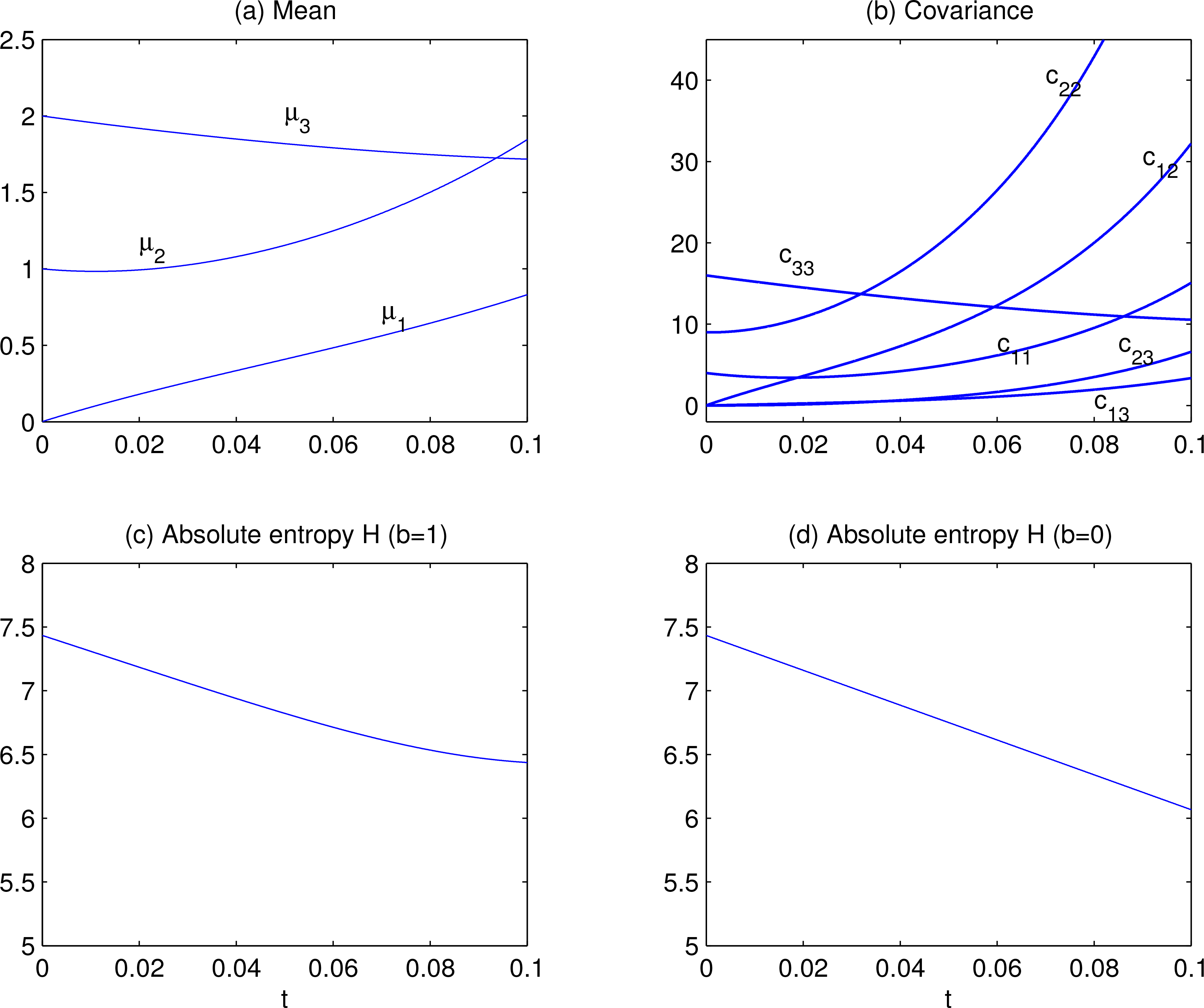
with b a tunable parameter. When b = 0, the stochasticity is turned off. Initialize (24) and (25) with μ = (0, 1, 2)^T, and c₁₁ = 4, c₂₂ = 9, c₃₃ = 16, c_ij = 0 for all i ≠ j. The solutions of μ and C are shown in Figure 1a,b. Correspondingly the absolute entropy H is plotted in Figure 1c,d is the entropy evolution of the corresponding deterministic system, i.e., b = 0. In this case, it is a straight line, with intercepts at t = 0 and t = 0.1 being 7.4335 and 6.0668, respectively, yielding a slope of

$$\frac{6.0668-7.4335}{0.1}=-13.667$$

On the other hand,

$$\nabla \cdot \mathbf{F}=Tr\left(\mathbf{A}\right)=-\left(\sigma +1+\beta \right)$$

and

$$\nabla \left(\text{log}\rho \right)=-\frac{1}{2}\nabla {\left(\mathbf{x}-\mathit{\mu }\right)}^T{\mathbf{C}}^{-1}\left(\mathbf{x}-\mathit{\mu }\right)=-{\mathbf{C}}^{-1}\left(\mathbf{x}-\mathit{\mu }\right)$$

which gives ∇[∇(log ρ)] = −C⁻¹. So, by the formula (11),

$$\frac{dH}{\mathit{dt}}=-\left(\sigma +1+\beta \right)+\frac{b^2}{2}\left(\tilde{\mathbf{B}}{\tilde{\mathbf{B}}}^T\right):{\mathbf{C}}^{-1}.$$

With the computed covariances, H can be integrated out, and the result is the same as that in Figure 1c (not shown). Particularly, when b =0, the slope of H is a constant, i.e., −(σ +1+ β) = 13.667, which is precisely what we obtained above in Figure 1d. With this linear system, the formula (11) and, particularly, Equation (5), is thence verified.

It should be noted that, in Figure 1d, the absolute entropy decreases linearly with time. Sooner or later it will hit the abscissa and become negative. This is a well-known fact for differential entropy, to which we limit our study. A simple example can illustrate this: Let x obey a uniform distribution on (0, $\frac{1}{2}$), then H = − log 2 < 0.

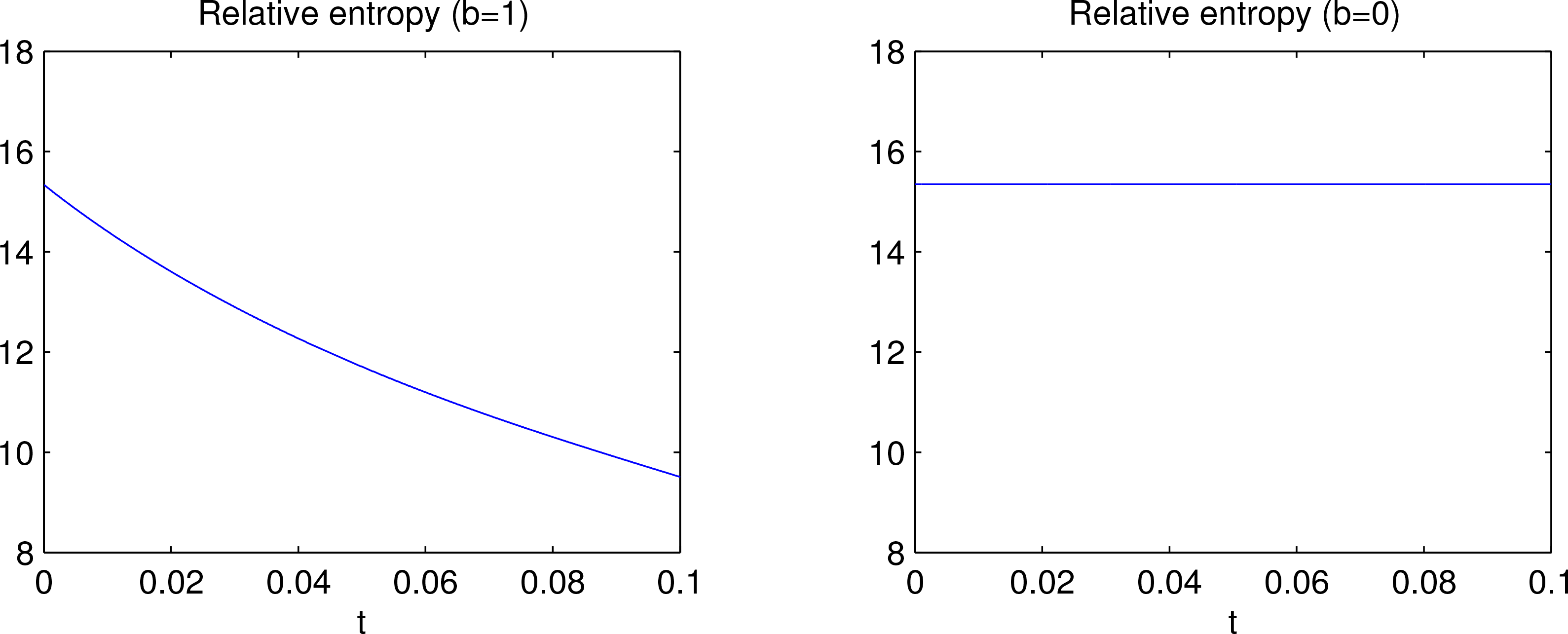
To see the relative entropy evolution, choose a mean vector and covariance matrix for the initial reference density:

$${\mathit{\mu }}_q\left(0\right)=\left(\begin{array}{c}1\\ -1\\ -2\end{array}\right),\hspace{0.17em}\hspace{0.17em}\hspace{0.17em}\hspace{0.17em}\hspace{0.17em}\hspace{0.17em}\hspace{0.17em}{\mathbf{C}}_q\left(0\right)=\left[\begin{array}{ccc}25& 0& 0\\ 0& 4& 0\\ 0& 0& 1\end{array}\right].$$

Then the relative entropy D evolution with time is shown as in Figure 2. Particularly, when the stochasticity is turned off, then D = 15.35 is a constant. This is precisely what the law on relative evolution, viz., Equation (8), would state for any deterministic systems.

5. Lorenz System

We now turn to the Lorenz system,

$$\frac{d{x}_1}{\mathit{dt}}=\sigma \left(x_2-x_1\right),$$

(30)

$$\frac{d{x}_2}{\mathit{dt}}=x_1\left(\rho -x_3\right)-x_2,$$

(31)

$$\frac{d{x}_3}{\mathit{dt}}=x_1{x}_2-\beta x_3,$$

(32)

which has a vector field

$$\mathbf{F}\left(\mathbf{x}\right)={\left[\sigma \left(x_2-x_1\right),x_1\left(\rho -x_3\right)-x_2,x_1{x}_2-\beta x_3\right]}^T.$$

We need to find its absolute entropy evolution. As normal, look at its density evolution first.

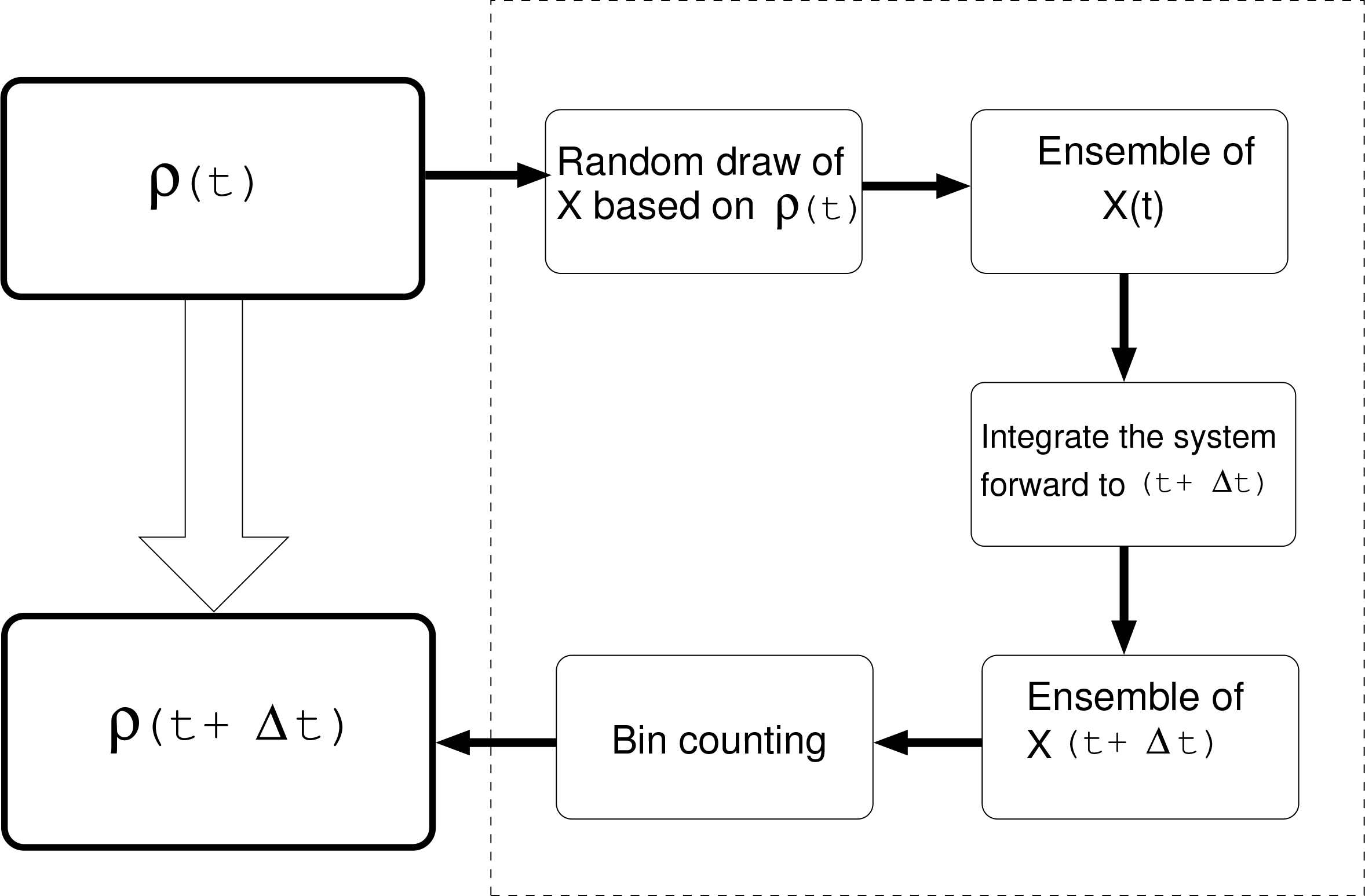
Different from the above linearized counterpart, the system is nonlinear and hence does not carry a probability density distribution known in form a priori as time moves on. To compute the density ρ, one naturally thinks of solving the Liouville Equation (4). This could be realized using a basis set or modes over its support, or numerical methods. An alternative but much more convenient and less expensive way is through ensemble prediction. As schematized in Figure 3, in order to predict ρ(t +Δt), given that all information at t is known, an ensemble prediction does not seek the solution from the Liouville Equation (4); rather, it makes a detour through the steps shown in dashed box. Both these techniques namely the Liouville equation method and ensemble prediction method are equivalent, but the former is way more expensive in terms of computation.

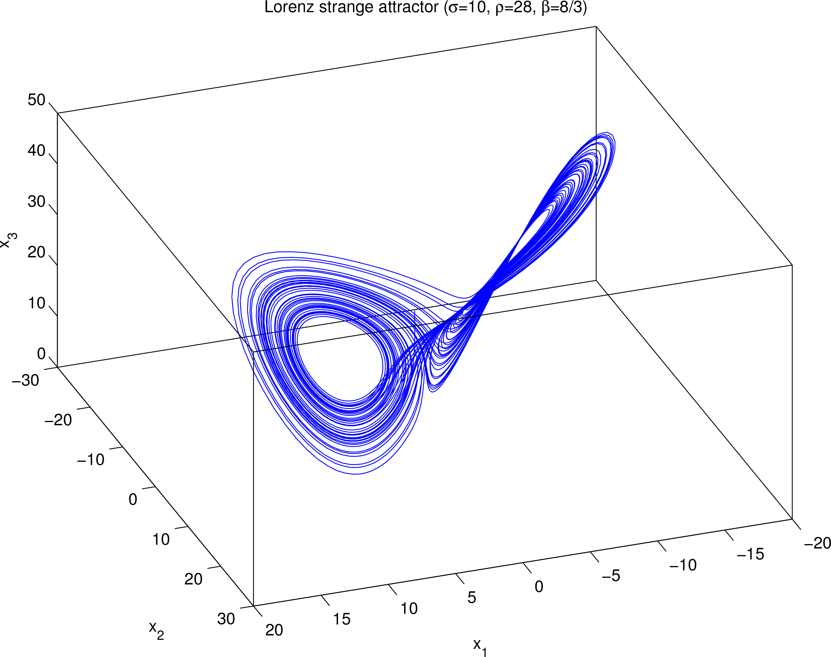
Figure 4 is the trajectory of Equations (30)–(32) starting at (6, 5, 30), with a time interval Δt = 0.01. The butterfly-like strange attractor demarcates the bounds for the 3D vector x: −17 < x₁ < 22, −22 < x₂ < 30, 0 < x₃ < 55. Thus it suffices to consider a sample space:

$$\Omega =\left[-25,35\right]\times \left[-25,35\right]\times \left[-2,58\right]$$

for all the trajectories, at least after enough long time of integration. We now discretize the sample space equally, with 101 grid points in each dimension, forming 100³ or one million cubic bins. Make random draws according to a normal distribution

$$N\left(\left[\begin{array}{c}0\\ 1\\ 28\end{array}\right],\hspace{0.17em}\hspace{0.17em}\hspace{0.17em}\left[\begin{array}{ccc}4& 0& 0\\ 0& 9& 0\\ 0& 0& 16\end{array}\right]\right)$$

so as to ensure that there are 161 draws for each dimension (which totals more than four million draws). Just as in the preceding section, the means are not essential; we choose μ = (0, 1, 28)^T for the convenience of computation, as it lies near the center of the attractor. We then integrate the system forward with a time step Δt = 0.01, and at each step count the bins with a population of 161³ ensemble members. The resulting density distribution is then used to estimate the absolute entropy H.

The computed H versus time is plotted in Figure 5 (thick solid line). Clearly, in the early stage of evolution, say, as t < 0.15, H declines linearly, with a slope of approximately −14, the same as that in the linear model (see Figure 1d). But beyond that, the trend is gradually reversed and then oscillates afterwards. To see how resolution of the sample space may affect the results, we try a low resolution, with only 51 grid points in each dimension (keep the same number of draws). The result is plotted in the figure as thin dashed lines. Apparently, the linear trend is also seen, but broken earlier. In another experiment, we increase the resolution so that there are 141 grid points in each dimension and, correspondingly, increase the number of random draws to 181 for each dimension, which totals almost 6 million draws. The result, however, is almost the same as that in the standard experiment. It seems that the absolute entropy shown as the solid line in Figure 5 is what we can get through numerical computation.

The above result, however, is at odds with what Equation (5) predicts. In the preceding section the Lorenz equations are linearized and the corresponding joint absolute entropy H is found to decrease with time at a constant rate (cf. Figure 1d). In fact, this is a property of the Lorenz system:

$$\frac{dH}{\mathit{dt}}=E\left(\nabla \cdot \mathbf{F}\right)=-\left(\sigma +1+\beta \right)=\text{const}.$$

(33)

Since the parameters σ, ρ, β are normally assumed to be positive (e.g., σ = 10, ρ = 28, β = 8/3, the values originally chosen by Lorenz), H will be on the decline forever. So, what is wrong here with the computation?

As discussed in the previous section, if H keeps decreasing at the same rate, sooner or later it will cross the abscissa and become negative. A problem arises at this junction. While the differential absolute entropy H admits negative values (see the example of uniform distribution in the preceding section), its discrete counterpart does not. If P_i is the probability for state i, one has

$$-\sum _i{P}_i\text{log}{P}_i\ge 0$$

(see Cover and Thomas, 1991). In discretizing the sample space for density estimation, one actually changes the problem of finding differential entropy into finding discrete entropy through bin counting. This is doomed to fail as the H approaches zero. As we have seen above, increasing the resolution of the sample space does help, either, since there is no way for discretized entropy to cross the abscissa! In this case, caution should be used when entropy is estimated using the technique of ensemble prediction and the subsequent bin-counting, particularly with real atmosphere-ocean problems, where this has been a widely accepted and efficient technique. This example tells us that, if absolute entropy H is computed, the concise formula (5) should be preferred.

6. Application to a Large-Dimensional Problem

We now consider a large-dimensional system, a fluid flow system. This kind of problems, which are described by partial differential equations (PDEs), are essentially of infinite size. But if we instead look at their numerical models, the dimensionality becomes finite, though very large in general. This section supplies a demonstration how the above formulas, namely, Equations (5), (8), (12), (14) and (15), may be applied to such a system. The purpose here is two-fold: The first is to provide a concrete example with technical details; the second is, in demonstrating the application, to look at how the uncertainty of the originally deterministic system is influenced after some stochasticity is added. For the former, we specifically need to

• Form the dynamical system;
• Find a way to initialize the system so as to get a chaotic attractor (only some particular pattern can destabilize the system);
• Drive the system toward a statistical equilibrium;
• Perform an EOF analysis to reduce the model to a low-dimensional system;
• Make random draws with the reduced model;
• Perform ensemble forecasts;
• Compute the entropy evolution using the above laws.

These will be shown in sequel in the following.

On the physics side, the motivation comes from the recent surge of interest in stochastic modeling of geophysical fluid flows–atmospheric and oceanic circulations. Realizing that model inaccuracy is inevitable (for example, it is impossible to accurately specify the boundary conditions in a weather forecast model), people have been turning their attention to stochastic PDEs, or SPDEs, with a stochastic term replacing the poorly represented physics in the governing equations (e.g., [33]). On the other hand, fluid flows are in general multiscale interactive. The atmospheric system, for example, contains millions of scales, from millimeters to tens of thousands kilometers, which cannot be all resolved in a computer model; the effect of the unresolved or subgrid processes must be parameterized for a reliable modeling. A promising approach to the parameterization problem is stochastic closure, which has been of great interest recently (e.g., [34,35]). All these concern of adding stochasticity to the original deterministic equations; it would be of interest to see how uncertainty may change when a system is changed from deterministic to stochastic.

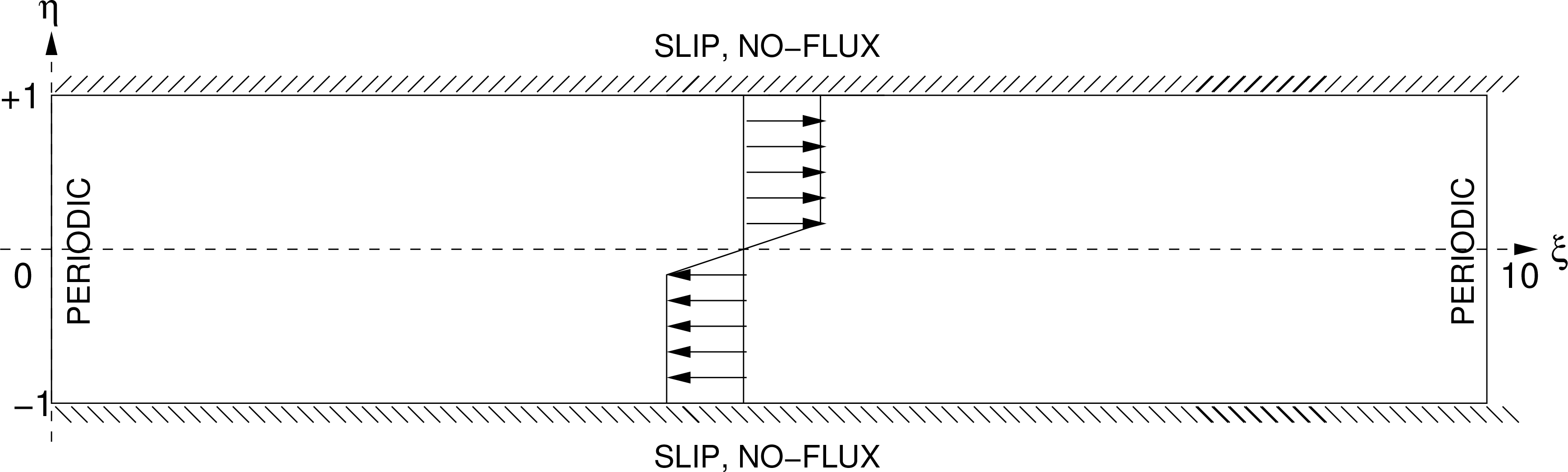
Consider a flow with a model domain as schematized in Figure 6. For the sake of simplicity, the study is limited to a horizontal flow, with independent variables ξ and η. (We write this way, instead of the conventional (x, y), to avoid confusion in notation.) Further, assume that the flow is quasi-geostrophic, so that only one state variable, namely, streamfunction, is needed (cf. [36,37]). Consider the perturbation from a zonal basic flow (U, V) = (U(η), 0), and define a perturbation streamfunction ψ such that $u=-\frac{\partial \psi }{\partial \eta }$, $v=\frac{\partial \psi }{\partial \xi }$ where (u, v) is the perturbation velocity. The SPDE of concern is

$$\frac{\partial ℒ\psi }{\partial t}=-\alpha \left(\frac{\partial \psi }{\partial \xi }\frac{\partial ℒ\psi }{\partial \eta }-\frac{\partial \psi }{\partial \eta }\frac{\partial ℒ\psi }{\partial \xi }\right)-U\frac{\partial ℒ\psi }{\partial \xi }-\left(\beta -U_{\eta \eta }\right)\frac{\partial \psi }{\partial \xi }+𝒦h\left(\xi ,\eta \right)\dot{w}.$$

(34)

Here $ℒ$ is the Laplacian operator: $ℒ$ = ∂²/∂ξ² +∂²/∂η², $𝒦$ a preset linear operator, h a given function of (ξ, η), and w˙ white noise with respect to some given filtration {$ℱ$_t}_t≥0. The boundary conditions are such that at η = ±1, ψ =0 (slip boundaries), and ξ =0 and ξ =10 are periodic. For simplicity, h is taken to be a constant. In this section two types of stochasticity are considered according to the operator $𝒦$ : (1) $𝒦$ = $ℒ$ ⁻¹; (2) $𝒦$ = 1. The first means that stochasticity applies to the streamfunction at each location, while in the second case stochasticity comes in with the vorticity equation at each location. In forming the discretized version large-dimensional system, the former results in a diagonal matrix B = hE in Equation (9); the latter leaves a B = hL⁻¹, where L is the discretized version of the Laplacian $ℒ$ .

The deterministic counterpart of the above SPDE is the barotropic quasi-geostrophic perturbation evolution equation in the absence of external forcing and friction. It and can be found in, say [37]. Its discretization is referred to [38], Appendix B.

We choose the shear instability model for our demonstration purpose. This extensively studied model has a velocity profile with a constant shear in the neighborhood of the axis, and zero elsewhere. Specifically, let

$$U\left(\eta \right)=\{\begin{array}{ll}1,\hfill & \hfill \eta >0.15\\ -1+\frac{20}{3}\left(\eta +0.15\right),\hfill & \hfill -0.15\le \eta \le 0.15\\ -1,\hfill & \hfill \eta <-0.15\end{array}$$

With this background flow we investigate the entropy evolution for the system (34). The forming of the large-dimensional system follows what we did in [38]. First, the domain as shown in Figure 6 is discretized into a grid with 80 × 40 cells; next Equation (34), together with the boundary conditions, is discretized on the grid using the central difference scheme. Invert the Laplacian and we then obtain the system. Specifically, Equation (34) is now replaced by its difference form:

$$\begin{array}{lll}L\frac{d{\psi }_{i,j}}{\mathit{dt}}\hfill & =\hfill & -\alpha \left(\frac{{\psi }_{i+1,j}-{\psi }_{i-1,j}}{2\Delta \xi }\times \frac{{\left(ℒ\psi \right)}_{i,j+1}-{\left(ℒ\psi \right)}_{i,j-1}}{2\Delta \eta }-\frac{{\psi }_{i,j+1}-{\psi }_{i,j-1}}{2\Delta \eta }\times \frac{{\left(ℒ\psi \right)}_{i+1,j}-{\left(ℒ\psi \right)}_{i-1,j}}{2\Delta \xi }\right)\hfill \\ \hfill & \hfill & -U_j\times \frac{{\left(ℒ\psi \right)}_{i+1,j}-{\left(ℒ\psi \right)}_{i-1,j}}{2\Delta \xi }-\left(\beta -U_{\eta \eta ,j}\right)\times \frac{{\psi }_{i+1,j}-{\psi }_{i-1,j}}{2\Delta \xi }+K{h}_{i,j}{\dot{w}}_{i,j}\hfill \\ \hfill & \equiv \hfill & N_{i,j}+K{h}_{i,j}{\dot{w}}_{i,j},\hfill \end{array}$$

(35)

where

$${\left(ℒ\psi \right)}_{i,j}=\frac{{\psi }_{i+1,j}-2{\psi }_{i,j}+{\psi }_{i-1,j}}{\Delta {\xi }^2}+\frac{{\psi }_{i,j+1}-2{\psi }_{i,j-1}}{\Delta {\eta }^2},$$

N_i,j is a nonlinear function of ψ and $ℒ$ ψ at the five grid points (i + 1, j), (i, j), (i − 1, j, (i, j + 1), (i, j − 1), and L and K are, respectively, the discretized forms of $ℒ$ and $𝒦$ . Left multiplication by L⁻¹, together with the boundary conditions, yields a stochastic dynamical system in the desired form:

$$\frac{d{\psi }_{i,j}}{\mathit{dt}}=L^{-1}N+L^{-1}K{h}_{i,j}{\dot{w}}_{i,j}.$$

(36)

In this study, the two parameters α = 2 and β = 1 are used.

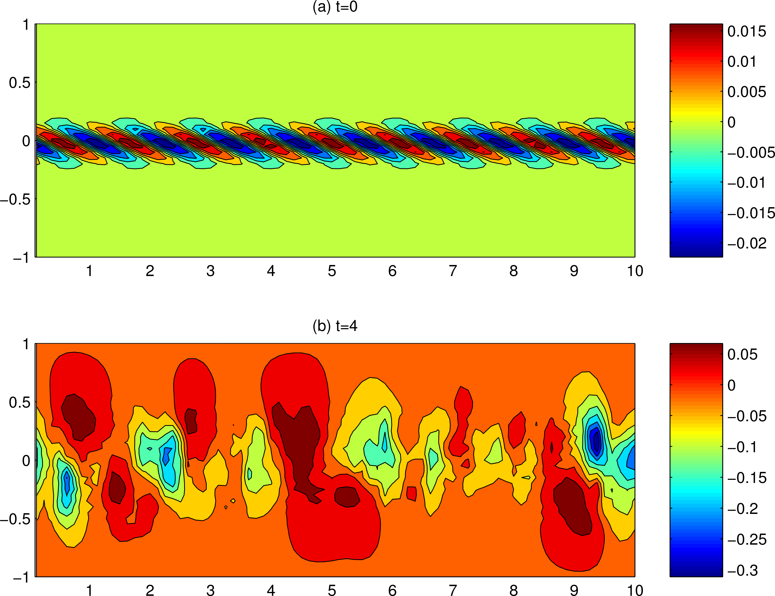
We look at how entropy evolves after the flow loses its stability and becomes chaotic. The first issue is how the integration should be initialized—different initializations will generally give different predictions, and not just any initialization may destabilize the flow. Here we use the optimal perturbation technique of [39] to find the optimal excitation mode (for details, see [38]). This mode is plotted in Figure 7a, where the perturbation amplitude is chosen to be 0.02. Once initialized, the deterministic model is integrated forward until it reaches a quasi-equilibrium, as shown in the chaotic state of Figure 7b.

The second issue is how the ensemble may be generated. Different from the Lorenz system as shown before, the dimensionality is huge here, and the ensemble generation method cannot be applied directly. To solve this problem, we use the empirical orthogonal function (EOF) technique [40] to reduce the system size. Starting from the chaotic state shown in Figure 7b, the model is further integrated for 5000 steps (or a duration t = 1.25 with time step Δt = 2.5 × 10⁻⁴), to form a time sequence of the ψ distribution.

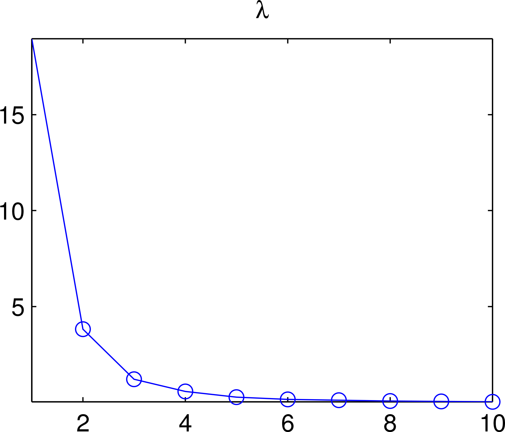
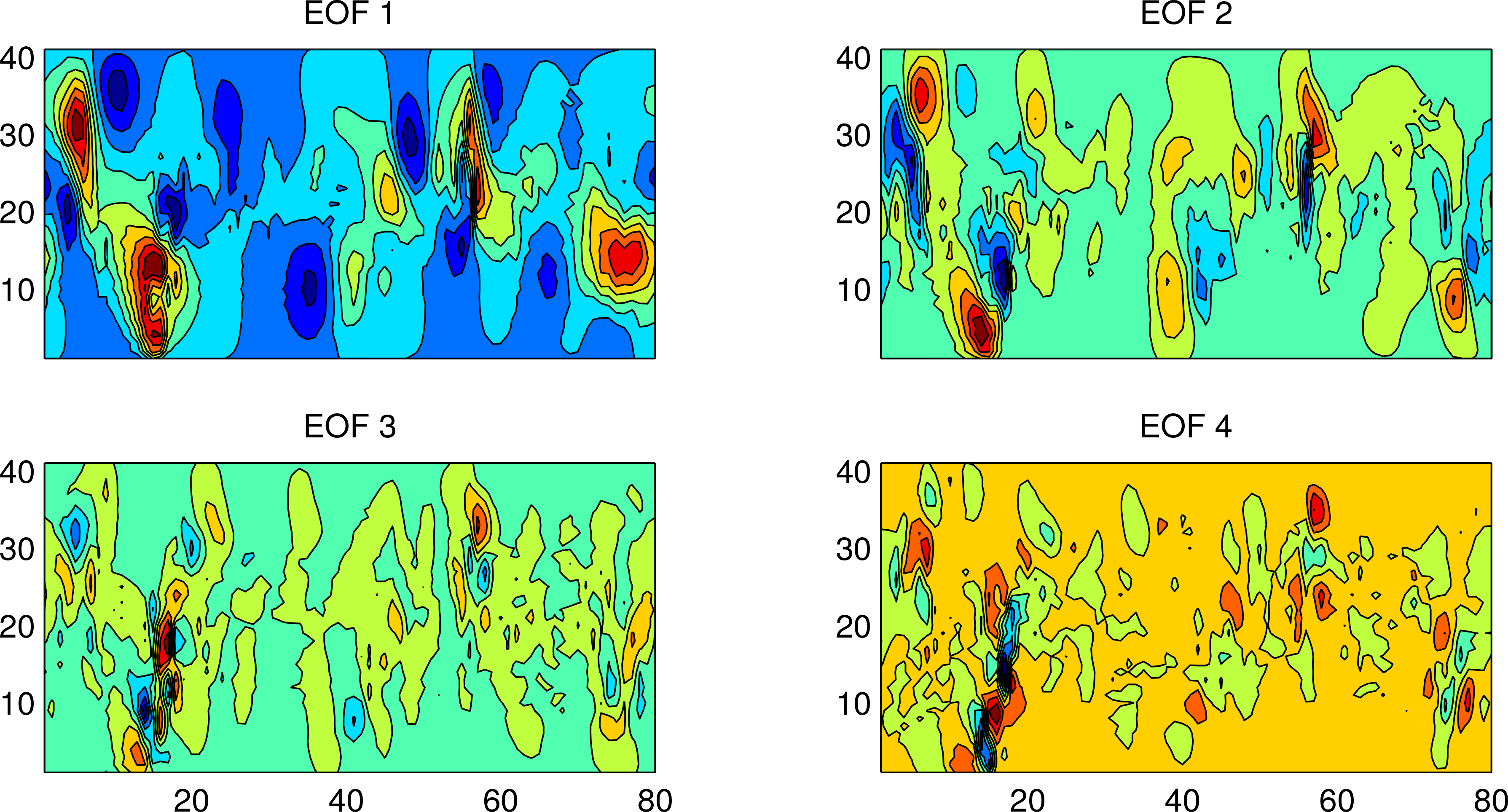
With the time sequence we perform the EOF analysis. Shown in Figure 8 are the variances associated with the modes. By calculation the first three account for 95% of the total variance; that is to say, the system essentially has a dimensionality of 3, rather than 80 × 40 = 3200. For safety, we choose 1 more mode to generate the ensemble. Shown in Figure 9 are these four modes.

We make random draws according to a joint Gaussian distribution of the above four modes. We use the Gaussian distribution not just because of its simplicity, but also because of the observation that, in a large system after sufficiently large number of iterates, the resulting distribution tends to be a Gaussian, thanks to the central limit theorem. Besides, given mean and variance, a distribution that maximizes absolute entropy must be a Gaussian. For convenience, let initially the four modes be uncorrelated so that we may consider each dimension independently (for a Gaussian, uncorrelatedness is equivalent to independence). From the time-varying coefficients in the above EOF analysis, the means and variances (μ_i,σ_i) for the four modes are estimated as: (0, 3.8 × 10⁻²), (0, 7.6 × 10⁻³), (0, 2.4 × 10⁻³), (0, 1.1 × 10⁻³), and the distributions are formed accordingly. We make five draws in each dimension; this yields an ensemble with a total of 5⁴ = 625 members.

For each member of the ensemble, the state is steered forth by the stochastic system; for simplicity, the stochastic perturbation amplitude is set to be a constant h = 0.01. This results in an ensemble, and hence a distribution, at each time step. As an example, shown in Figure 10a is a snapshot of the computed histogram of ψ at point (70, 25). An observation about the distributions: the spread growth is inhomogeneous in space; actually at some points it may not grow at all, though it is generally believed that, for a weather system, any prediction tends to deteriorate rapidly. In order to examine the impact of stochasticity perturbation, a model run with h =0 is launched. For comparison, we draw the histograms of ψ at some points; shown in Figure 10b is an example at (70, 25). The interesting thing here is, though stochasticity literally means uncertainty, at some points the spread of ψ with the stochastic system is slower than that with the corresponding deterministic system. Spread alone, of course, is not enough to characterize the uncertainty. We next estimate the entropy evolution. Note that the initial condition H(0) = const does not affect our study of the evolution of H(t), this constant can be anything.

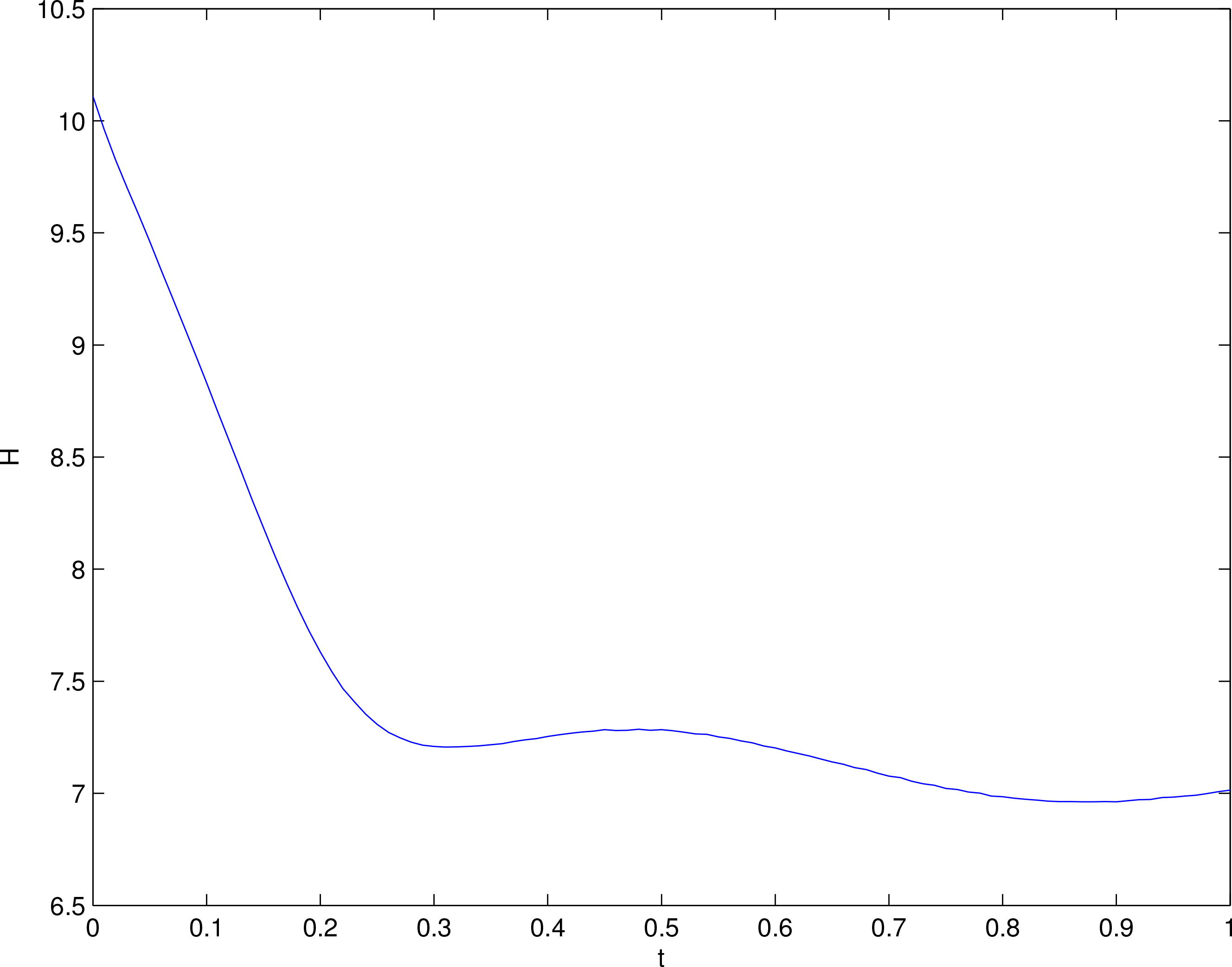
The computed entropy evolutions with the deterministic and stochastic systems are shown in Figure 11, where the blue curve stands for the case h = 0, and the green curve for h = 0.01. Different from its relative entropy counterpart, the absolute entropy H does not need to grow as stochasticity comes in. In the figure this is particularly clear around t = 0.1, where the entropy of the deterministic case attains a local maximum but that of the stochastic system is a minimum. Obviously, stochasticity does not always leave a system more uncertain.

The phenomenon of uncertainty reduction, albeit seemingly counterintuitive, actually can be understood from the formulas. By Equations (8) and (15), a deterministic system conserves its relative entropy D, and stochasticity reduces it. That is to say, stochasticity always causes a system to lose predictability. This is the natural result that one would expect. For absolute entropy H, one may also argue, based on a comparison of Equation (12) to (5), that stochasticity increases H and hence uncertainty. This, unfortunately, need not always be true. The issue here is, the part E(∇·F) in the two formulas are not the same thing; when stochasticity is introduced, E(∇·F) may vary accordingly—it may rise or fall. If it falls, the decrease could surpass the increase due to the stochastic process, resulting in a deficit in absolute entropy, and hence a reduced uncertainty. This is what is shown in the above model result.

7. Discussion

We have presented a comprehensive introduction and a systematic derivation of the evolutionary laws for absolute entropy H and relative entropy D with respect to dynamical systems, both deterministic and stochastic, and explored applications to the renowned Lorenz system and a large-dimensional system namely a stochastic fluid flow problem. For easy reference, the resulting formulas are wrapped up in the following.

If a deterministic system

$$\frac{d\mathbf{x}}{\mathit{dt}}=\mathbf{F}\left(\mathbf{x},t\right)$$

(37)

is considered, its absolute entropy H and relative entropy D evolve as:

$$\frac{dH}{\mathit{dt}}=E\left(\nabla \cdot \mathbf{F}\right),$$

(38)

$$\frac{dD}{\mathit{dt}}=0.$$

(39)

If the system has stochasticity included:

$$d\mathbf{x}=\mathbf{F}\left(\mathbf{x},t\right)dt+B\left(\mathbf{x},t\right)d\mathbf{w},$$

(40)

then

$$\frac{dH}{\mathit{dt}}=E\left(\nabla \cdot \mathbf{F}\right)-\frac{1}{2}E\left(\mathbf{G}:\nabla \nabla {\ell }_p\right),$$

(41)

$$\frac{dD}{\mathit{dt}}=-\frac{1}{2}E\left[\nabla {\ell }_{\rho /q}\cdot \mathbf{G}\cdot \nabla {\ell }_{\rho /q}\right],)$$

(42)

where ℓ_ρ = log ρ, ℓ_ρ/q = log ρ/q, and G = BB^T . In Equation (40), if B has no dependence on x, in other words, if the noise is additive, then

$$\frac{dH}{\mathit{dt}}=E\left(\nabla \cdot \mathbf{F}\right)+\frac{1}{2}E\left(\nabla {\ell }_{\rho }\cdot \mathbf{G}\cdot \nabla {\ell }_{\rho }\right).$$

(43)

Moreover, if the parameters, say, the means μ_i, of the pdf are bound to the state variables in a form of translation (as that in a Gaussian), then the above formula is further reduced to

$$\frac{dH}{\mathit{dt}}=E\left(\nabla \cdot \mathbf{F}\right)+\frac{1}{2}\mathbf{G}:\mathbf{I},$$

(44)

where I = (I_ij) is the Fisher information matrix.

Among the above Equations (38), (39) and (41)–(44), Equations (41), (43) and (44) are new. Equation (42) is a generalization of that in [30] with their positivity assumption relaxed. Since a mathematical expectation may be well estimated by an ensemble mean, and there are many ways to estimate I⁻¹ the Cramér–Rao bound, Equation (44) enables us to avoid the expensive yet inaccurate pdf estimation in investigating the uncertainty evolution in large-dimensional systems.

For a linear system

$$d\mathbf{x}=\mathbf{A}x+\mathbf{B}d\mathbf{w},$$

(45)

the above formulas can be explicitly written out in terms of means and covariances. Here x = (x₁, x₂, ..., x_n)^T, and A and B are constant matrices. For such as system, if initially x is Gaussian-distributed, it will keep being a Gaussian forever. Let the mean vector be μ and covariance matrix be C. Then

$$H=\text{log}\left[{\left(2\pi \right)}^{n/2}{\left(\text{det}\hspace{0.17em}\mathbf{C}\right)}^{1/2}\right]+\frac{n}{2}.$$

(46)

$$D=\frac{1}{2}\text{log}\left(\frac{{\text{det}\hspace{0.17em}\mathbf{C}}_q}{\text{det}\hspace{0.17em}\mathbf{C}}\right)-\frac{n}{2}+\frac{1}{2}\mathbf{C}:{\mathbf{C}}_q^{-1}+\frac{1}{2}{\left(\mathit{\mu }-{\mathit{\mu }}_q\right)}^T{\mathbf{C}}_q^{-1}\left(\mathit{\mu }-{\mathit{\mu }}_q\right),$$

(47)

where μ_q and C_q are the means and covariances of the reference distribution. Subsequently we have the time rate of change of H and D

$$\frac{dH}{\mathit{dt}}Tr\left(\mathbf{A}\right)+\frac{1}{2}\left({\mathbf{BB}}^T\right):{\mathbf{C}}^{-1},$$

(48)

$$\frac{dD}{\mathit{dt}}=\left({\mathbf{BB}}^T\right):{\mathbf{C}}_q^{-1}-\frac{1}{2}\left({\mathbf{BB}}^T\right):\left({\mathbf{C}}^{-1}+{\mathbf{C}}_q^{-1}{\mathbf{CC}}_q^{-1}\right)-\frac{1}{2}{\left(\mathit{\mu }-{\mathit{\mu }}_q\right)}^T{\mathbf{C}}_q^{-1}{\mathbf{BB}}^T{\mathbf{C}}_q^{-1}\left(\mathit{\mu }-{\mathit{\mu }}_q\right).$$

(49)

Particularly, in the absence of stochasticity, $\frac{dH}{\mathit{dt}}$ can be obtained without solving the governing equation or the equation for μ and C: dH/dt = Tr (A) . In this case, the time rate of absolute entropy change is precisely equal to the trace of A. For relative entropy, we recover the conservation law, i.e., dD/dt = 0. These results have been tested with a specific linear system.

One may ask about how the result may comply to the second law of thermodynamics. As discussed extensively before [21,25], relative entropy is always dissipated and non-increasing, in accordance to the law; Equation (42) particularly shows that its dissipative representation in the equation has a form reminiscent of the Fisher information. The absolute entropy, in contrast, need not be increasing all the time (see below for a specific example). It is a proved fact in probability theory that a distribution that maximizes absolute entropy unconditionally must be uniform. One may argue that, if initially a system has a uniform distribution, then it cannot change any more, otherwise the entropy will fall as time goes on, violating the above second law. This is, of course, not true in reality, and hence absolute entropy need not increase with a dynamical system. This, however, does not mean that the second law of thermodynamics is violated. What the second law states applies to isolated systems, excluding the possibility of phase space expansion or contraction. When the conformity between the law and Equation (41) is discussed, it would be more appropriate to limit the discussion to divergence-free systems like the Hamiltonian systems. (Recently, the second law is generalized for open systems; see the fluctuation theorem in [41].)

We have put the obtained evolutionary laws to application to the renowned Lorenz system, and a large-dimensional system. The Lorenz system, though highly nonlinear, actually has a constant vector field divergence, and the constant is negative. By Equation (38), this implies a constantly decreasing absolute entropy H. That is to say, on a plot of H versus time, sooner or later it will hit the abscissa and become negative, no matter how it is initialized. Though absolute entropy in the discrete sense is always above or equal to zero, a negative differential entropy is not uncommon; a simple example is a uniformly distributed random variable x on (0, $\frac{1}{2}$), which by calculation has an H = − log 2 < 0. The makes a big issue in computing uncertainties in ensemble prediction problems (such as weather forecasting), where sample space coarse-graining is a common practice. In these computations, statistical properties are estimated through counting the bins on the discretized sample space—The widely used histogram plot drawing is just such an exercise. The resulting estimate of H is, therefore, a discrete one, and hence can never go below zero. In this study we showed that, the H estimated through bin counting is relevant only on the short interval before it approaches zero. Here the moral is: when dealing with highly dissipative systems such as the Lorenz system, caution should be used in estimating its absolute entropy.

Heuristically, if we imagine a dynamical system with a point attractor then, when the system is deterministic, its ensemble density will shrink to a delta function over the point attractor. During this process, absolute entropy will decrease at a constant rate. If we now add stochastic fluctuations, at some point the contraction of phase space to the point attractor and the dispersive effect of fluctuations will balance and the absolute entropy will asymptote to a (usually negative) constant value (at the steady state solution of the Fokker–Planck equation). On the other hand, if we consider the relative entropy, for deterministic systems this will be conserved as time progresses. The addition of random fluctuations will, in contrast, render the initial distributions indistinguishable, making the relative entropy fall to its lower bound of zero as the ensemble converges on the point attractor.

The application of the formulas requires ensemble prediction, and this is computationally tractable only for low-dimensional systems (as the above Lorenz system). To see how this may work for large-dimensional systems, we examined a stochastic quasi-geostrophic flow model. Stochastic modeling is hot these days in oceanography and atmospheric science, partially reflecting the effort to recover the unresolved small-scale processes and to remedy the model inaccuracies. In this study we particularly investigated through a shear-instability problem how the addition of stochasticity may change the uncertainty of the system which would otherwise be deterministic. Initialized with an optimal excitation perturbation, the pattern appears chaotic. To see how its uncertainty evolves, first we reduced the model to a computationally tractable 3D problem, using the EOF analysis, then generated an ensemble with respect to the resulting EOF modes. The above formulas, after being applied to this ensemble and the vector field derived from the discretized system, yield an absolute entropy oscillating with time. An interesting observation is that, though stochasticity has almost been taken as a synonym of uncertainty, it does not necessarily leave a system more uncertain. In fact, sometimes introduction of noise may reduce the uncertainty of the system!

Uncertainty reduction due to noise addition occurs in a system when the reduction in phase volume expansion exceeds the uncertainty that the noise brings in. In Equation (41), that is to say, the reduction of E(∇ · F) exceeds the reduction of $\frac{1}{2}E\left(\mathbf{G}:\nabla \nabla \text{log}{\ell }_{\rho }\right)$. For this reason, uncertainty reduction does not happen just under any circumstances. First, it is not permissible in linear systems. By Equation (48), a linear system always has a constant ∇ · F. For example, the most common mean reverting stochastic process, Ornstein–Uhlenbeck process,

$$dx=\lambda \left(\mu -x\right)dt+\sigma dw$$

(50)

(λ > 0, σ > 0, and μ are parameters), has a constant divergence −λ. There is no way to have it decreased with the addition of σdw in the equation. Clearly, uncertainty reduction can only occur in nonlinear systems.

Nonlinearity, however, is not a sufficient condition. The Lorenz system shown above is an example—albeit highly nonlinear, E(∇ · F) is always a constant. Another example is the Schwartz type 1 process, a popular stochastic process in finance:

$$dx=\kappa \left(\mu -\text{log}x\right)xdt+\sigma xdw.$$

(51)

Here E(∇ · F)= −κE(log x) − κ. This is not a constant, but depending on E(log x). However, the process is actually a log price Ornstein–Uhlenbeck process:

$$d\text{log}x=\kappa \left(\mu -\text{log}x\right)dt+\sigma dw,$$

and hence

$$\frac{dE\left(\text{log}x\right)}{\mathit{dt}}=\kappa \left(\mu -\text{log}x\right),$$

which gives an evolution of E(log x) independent of σ. That is to say, stochasticity exerts no effect on E(∇ · F); in this case uncertainty always rises when stochasticity is included.

The Lorenz system and the quasi-geostrophic flow system are examples of self-organization, a process with which a system spontaneously moves from more probable states towards states of low probability, and through which the system reduces its absolute entropy, via exchanging information with the outside world (e.g., [42]). Both systems show that self-organization is manifested in phase space contraction. The flow instability problem particularly shows that the white noise from without may facilitate this process, leading to a reduction of uncertainty in comparison to the corresponding deterministic case. Obviously, for this to happen, nonlinearity is a necessary, albeit not sufficient, condition. But how nonlinearity and stochasticity work together to fulfill a reorganization of otherwise random states is not clear. This is, of course, beyond the scope of the present study, which is only for a demonstrating purpose. We will follow that up in future investigations.

References

- Shannon, C.E. A mathematical theory of communication. Bell Syst. Tech. J. 1948, 27, 379–423. [Google Scholar]
- Jaynes, E.T. Information theory and statistical mechanics. PhysRev 1957, 106, 620–630. [Google Scholar]
- Georgescu-Roegen, N. The Entropy and the Economic Process; Harvard University Press: Cambridge, MA, USA, 1971. [Google Scholar]
- Lin, S.-K. Diversity and entropy. Entropy 1999, 1, 1–3. [Google Scholar]
- Maes, C.; Redig, F.; Moffaert, J. On the definition of entropy production via examples. MathPhys 2000, 41, 1528. [Google Scholar]
- Ruelle, D. How should one define entropy production for nonequilibrium quantum spin systems? MathPhys 2002, 14, 701–707. [Google Scholar]
- Jakšić, V.; Pillet, C.-A. A note on the entropy production formula. ContempMath 2003, 327, 175. [Google Scholar]
- Gallavotti, G. Entropy production in nonequilibrium stationary states: A point of view. Chaos 2004, 14, 680–690. [Google Scholar]
- Goldstein, S.; Lebowitz, J. On the (Boltzmann) entropy of nonequilibrium systems. Physica D 2004, 224, 53–66. [Google Scholar]
- Tomé, T. Entropy production in nonequilibrium systems described by a Fokker–Planck equation. Braz. J. Phys 2006, 36, 1285–1289. [Google Scholar]
- Pavon, M.; Ticozzi, F. On entropy production for controlled Markovian evolution. J. Math. Phys 2006, 47, 1–11. [Google Scholar]
- Polettini, M. Fact-checking Ziegler’s maximum entropy production principle beyond the linear regimes and towards steady states. Entropy 2013, 15, 2570–2584. [Google Scholar]
- Martyushev, L.M. Entropy and entropy production: Old misconceptions and new breakthroughs. Entropy 2013, 15, 1152–1170. [Google Scholar]
- Lorenz, E. A study of the predictability of a 28-variable atmospheric model. Tellus 1965, 17, 321–333. [Google Scholar]
- Epstein, E.S. Stochastic dynamic prediction. Tellus 1969, 21, 739–759. [Google Scholar]
- Leith, C.E. Theoretical skill of Monte Carlo forecasts. MonWeather Rev 1974, 102, 409–418. [Google Scholar]
- Ehrendorfer, E.; Tribbia, J. Optimal prediction of forecast error covariances through singular vectors. J. AtmosSci 1997, 54, 286–313. [Google Scholar]
- Moore, A.M. The dynamics of error growth and predictability in a model of the Gulf Stream. II. Ensemble prediction. J. PhysOceanogr 1999, 29, 762–778. [Google Scholar]
- Schneider, T.; Griffies, S.M. A conceptual framework for predictability studies. J. Clim 1999, 12, 3133–3155. [Google Scholar]
- Palmer, T.N. Predicting uncertainty in forecasts of weather and climate. Rep. ProgPhys 2000, 63, 71–116. [Google Scholar]
- Kleeman, R. Measuring dynamical prediction utility using relative entropy. J. AtmosSci 2002, 59, 2057–2072. [Google Scholar]
- Kirwan, A.D.; Toner, M.; Kantha, L., Jr. Predictability, uncertainty, and hyperbolicity in the ocean. Int. J. EngSci 2003, 41, 249–258. [Google Scholar]
- Lermusiaux, P.F.J. Uncertainty estimation and prediction for interdisciplinary ocean dynamics. J. Comput. Phys 2006, 217, 176–199. [Google Scholar]
- Evangelinos, C.; Lermusiaux, P.F.J.; Xu, J.; Haley, P.J.; Hill, C.N. Many task computing for real-time uncertainty prediction and data assimilation in the ocean. IEEE Trans. Parallel. DistrSyst 2011, 22, 1012–1024. [Google Scholar]
- Cover, T.M.; Thomas, J.A. Elements of Information Theory; Wiley: New York, NY, USA, 1991. [Google Scholar]
- Andrey, L. The rate of entropy change in non-Hamiltonian systems. PhysLett 1985, 111A, 45–46. [Google Scholar]
- Liang, X.S.; Kleeman, R. Information transfer between dynamical system components. Phys. Rev. Lett 2005, 95, 244101. [Google Scholar]
- Plastino, A.R.; Daffertshofer, A. Liouville Dynamics and the conservation of information. Phys. Rev. Lett 2004, 93, 138701. [Google Scholar]
- Liang, X.S. Local predictability and information flow in complex dynamical systems. Physica D 2013, 248, 1–15. [Google Scholar]
- Plastino, A.R.; Miller, H.G.; Plastino, A. Minimum Kullback entropy approach to the Fokker–Planck equation. Phys. Rev. E 1997, 56, 3927. [Google Scholar]
- Liang, X.S.; Kleeman, R. A rigorous formalism of information transfer between dynamical system components. I. Discrete mapping. Physica D 2007, 231, 1–9. [Google Scholar]
- Friston, K.; Ao, P. Free energy, value, and attractors. Comput. Math. Methods Med. 2012. [Google Scholar] [CrossRef]
- Duan, J.; Gao, H.; Schmalfu, B. Stochastic dynamics of a coupled atmosphere-ocean model. StochDyn 2002. [Google Scholar] [CrossRef]
- Majda, A.J.; Timofeyev, I.; Vanden-Eijnden, E. A mathematical framework for stochastic climate models. Commun. Pure Appl. Math 2001, 54, 891–974. [Google Scholar]
- Mana, P.G.L.; Zanna, L. Stochastic parameterization of ocean mesoscale eddies. Ocean Model 2014, 79, 1–20. [Google Scholar]
- Pedlosky, J. Geophysical Fluid Dynamics, 2nd ed; Springer: New York, NY, USA, 1979; p. 710. [Google Scholar]
- Vallis, G.K. Atmospheric and Oceanic Fluid Dynamics; Cambridge University Press: Cambridge, MA, USA, 2006; p. 745. [Google Scholar]
- Liang, X.S. Uncertainty generation in deterministic flows: Theory and application with an atmospheric jet stream model. Dyn. Atmos. Ocean 2011, 52, 51–79. [Google Scholar]
- Farrell, B.F.; Ioannou, P.J. Generalized stability theory. Part I. Autonomous operators. J. AtmosSci 1996, 53, 2025–2040. [Google Scholar]
- Preisendorfer, R.W. Principal Component Analysis in Meteorology and Oceanography; Elsevier: Amsterdam, The Netherlands, 1988. [Google Scholar]
- Evans, D.J. A non-equilibrium free energy theorem for deterministic systems. MolPhys 2003, 101, 1551–1554. [Google Scholar]
- Bar-Yam, Y. Dynamics of Complex Systems; Perseus Books: Reading, MA, USA, 1997; p. 848. [Google Scholar]
Figure 1.
The solution of Equations (24) and (25) with the parameters as specified in the text: (a) the means (b = 1); (b) the covariances (b = 1); (c) the absolute entropy H (b = 1). (d) H versus time for the corresponding deterministic system (b = 0); here H evolves as a straight line with a slope of −13.667.
Figure 2.
Relative entropy evolution with a stochastic system (left) and its corresponding deterministic system (right).
Figure 3.
Schematic of ensemble prediction. Given the density at t, ρ(t), one makes a detour as shown in the dashed line box to get the density at t+Δt, i.e., ρ(t+Δt), rather than obtains the latter directly from the Liouville equation.
Figure 4.
Solution of the Lorenz system (30)–(32) with Δt = 0.01. It is initialized at x0 = (6, 5, 30)T .
Figure 5.
Evolution of absolute entropy obtained through ensemble prediction and pdf estimation.
Figure 6.
Configuration of the shear instability model.
Figure 7.
Snapshots of ψ, the dimensionless perturbation streamfunction: (a) initial condition; (b) distribution at t = 4.
Figure 8.
Variance versus EOF modal number.
Figure 9.
Structures of the first four EOF modes. These modes are normalized.
Figure 10.
A snapshot of the histograms of the streamfunction at point (70, 25) predicted with the stochastic and deterministic systems: (a) stochastic system (h = 0.01); (b) deterministic system (h = 0).
Figure 11.
Evolution of absolute entropy H with the system (34) for h = 0.01 (green) and h = 0 (blue).
© 2014 by the authors; licensee MDPI, Basel, Switzerland This article is an open access article distributed under the terms and conditions of the Creative Commons Attribution license (http://creativecommons.org/licenses/by/3.0/).
Share and Cite
MDPI and ACS Style
Liang, X.S. Entropy Evolution and Uncertainty Estimation with Dynamical Systems. Entropy 2014, 16, 3605-3634. https://doi.org/10.3390/e16073605
AMA Style
Liang XS. Entropy Evolution and Uncertainty Estimation with Dynamical Systems. Entropy. 2014; 16(7):3605-3634. https://doi.org/10.3390/e16073605
Chicago/Turabian StyleLiang, X. San. 2014. "Entropy Evolution and Uncertainty Estimation with Dynamical Systems" Entropy 16, no. 7: 3605-3634. https://doi.org/10.3390/e16073605