Article

Accuracy of 3D Landscape Reconstruction without Ground Control Points Using Different UAS Platforms

1
Applied Remote Sensing Lab, Department of Geography, McGill University, Montreal, QC H3A 0B9, Canada
2
National Research Council of Canada, Flight Research Lab, Ottawa, ON K1A 0R6, Canada
3
Institut de recherche en biologie végétale, Université de Montréal, Montreal, QC H1X 2B2, Canada
4
Durham Regional Police, Whitby, ON L1N 0B8, Canada
*
Author to whom correspondence should be addressed.
Drones 2020, 4(2), 13; https://doi.org/10.3390/drones4020013
Submission received: 26 March 2020 / Revised: 20 April 2020 / Accepted: 20 April 2020 / Published: 24 April 2020
(This article belongs to the Special Issue She Maps)

Abstract

:
The rapid increase of low-cost consumer-grade to enterprise-level unmanned aerial systems (UASs) has resulted in the exponential use of these systems in many applications. Structure from motion with multiview stereo (SfM-MVS) photogrammetry is now the baseline for the development of orthoimages and 3D surfaces (e.g., digital elevation models). The horizontal and vertical positional accuracies (x, y and z) of these products in general, rely heavily on the use of ground control points (GCPs). However, for many applications, the use of GCPs is not possible. Here we tested 14 UASs to assess the positional and within-model accuracy of SfM-MVS reconstructions of low-relief landscapes without GCPs ranging from consumer to enterprise-grade vertical takeoff and landing (VTOL) platforms. We found that high positional accuracy is not necessarily related to the platform cost or grade, rather the most important aspect is the use of post-processing kinetic (PPK) or real-time kinetic (RTK) solutions for geotagging the photographs. SfM-MVS products generated from UAS with onboard geotagging, regardless of grade, results in greater positional accuracies and lower within-model errors. We conclude that where repeatability and adherence to a high level of accuracy are needed, only RTK and PPK systems should be used without GCPs.

Graphical Abstract

1. Introduction

The recent rapid development of relatively low-cost (<US$25,000) small unmanned aerial systems (UASs) (<25 kg) has resulted in their use in a myriad of disciplines. Applications in precision agriculture [1,2], archeological reconstruction [3,4], forestry [5,6], geomorphology [7,8,9], freshwater and marine systems [10,11,12], environmental monitoring [13,14], animal population studies [15,16,17,18], and recently, traffic accident reconstruction [19,20] are just a few of the fields where UASs have been exploited and continue to grow with enhanced platform capabilities (e.g., real-time analysis) [21], advanced sensors [22,23,24] and diverse software implementations [25,26]. The high accuracy and precision (i.e., cm error) of results obtained for 2D (e.g., orthomosaics) and 3D (e.g., digital surface model—DSM) mapping, based on structure from motion with multiview stereo photogrammetry (SfM-MVS), is transforming most disciplines where studies need to characterize areas up to ~100 hectares [1,27,28]. In addition, more operationally demanding systems such as hyperspectral pushbroom sensors [22,29], thermal imagers [24] and LiDAR [30] are being implemented on UASs, providing new insights for data fusion and advanced data analysis [31]. Centimeter level accuracies are particularly important in these multi-sensor applications where spatial alignment of the different datasets is needed. At the moment, the vast majority of applications within the public-domain, are limited to small UASs with limited coverage due to the near-universal regulatory requirement that these systems be flown within visual-line-of-sight (VLOS) [32]. As well, limited battery performance [33] and a restricted envelop of weather conditions for operations compounds the current limitations of small UAS operations. However, as UAS technology matures and more robust operations such as beyond-visual-line-of-sight (BVLOS) become common [34], novel applications will continue to be tested [35]. It is important to recognize, however, that small UAS BVLOS is still in its early stages of development [36] and it will be some time before unfettered BVLOS operations will be allowed by airspace regulators. In these future BVLOS applications, using GCPs collected on-site will not always be a viable option because of the large extents that will be covered by the imagery and the potential remoteness or inaccessibility of the study area (e.g., [35,37]).
While the early development of SfM photogrammetry emerged approximately 40 years ago [38], its popularity in geomatics has increased with access to higher performance computers/workstations and the availability of UAS-based photography [39]. A generic SfM pipeline reconstructs the landscape as a sparse 3D point cloud from overlapping 2D photographs. Additional products such as a dense 3D point cloud (through the application of an MVS algorithm), a DSM from interpolation of the point cloud or a textured mesh can also be generated. The SfM algorithms locate common points in the multiple 2D photographs taken from different viewing positions (and angles) from which the landscape is reconstructed in 3D [40,41]. The SfM pipeline does not actually require any geopositioned information for the photographs. In the absence of coordinates, it recovers the camera parameters, and position and orientation estimates from the photographs resulting in more flexibility than conventional photogrammetry from stereo-pairs [42]. A review of different algorithms and implementations of SfM can be found in [43].
Many factors that affect the quality of the UAS-based SfM-MVS photogrammetry products (e.g., orthomosaic and DSM) are described in detail by [44,45]. The first consideration is the image size as defined by the number of pixels on the imaging sensor, namely the pixel size and pixel pitch (i.e., the linear distance from the center of a pixel to the center of the adjacent pixel on the detector array). The size of the detector array and the size of the pixels affect the resolving power of the sensor. Given a specific pixel size, larger arrays accommodate more pixels that capture more incoming electrons, but given a specific sensor size, larger pixels are a tradeoff in a corresponding loss of spatial resolution. The second factor is the sensor’s radiometric resolution (e.g., 8–14 bits), where a higher radiometric resolution corresponds to the system being able to accommodate a greater range of intensities of incoming radiation. A final important factor to consider is the accurate location of imaged features with respect to the real-world coordinates (absolute position) and accurate geometries (dimensions, distances and volumes) as they are represented in the products (relative accuracy). In addition, minimization of image blur and distortion for a given camera and lens implementation during mission planning requires the consideration of specific camera and lens parameters (e.g., f-stop, shutter speed and ISO) [44]. In addition to hardware specifics, several studies have addressed equally important aspects of data collection from UASs such as flight altitude [46,47], image overlap [48] and environmental conditions (i.e., wind speed) for optimizing data collection [22], which are closely related to the implementation’s objective(s).
However, positional accuracy is still a very challenging attribute to conceive and quantify for many UAS practitioners. The general lack of knowledge of true positional errors is in part, due to the relatively high degree of ease of collecting ultra-high-resolution (few cm) images. It has been recognized, previously, that UASs and their system implementation requires improvement [49,50]. Applications where high accuracy and/or precision (e.g., repeatability) are required, have relied on the use of ground control points (GCPs) for improving product geolocation with respect to real-world coordinates and for ensuring accurate measurements of geometries within the end-products (e.g., [51]). For instance, [52,53,54] have shown the utility of GCPs for improving horizontal and vertical positional accuracy for different data acquisition scenarios (e.g., GCP density and distribution). Nevertheless, as stated by [55], implementing a GCP network can be impractical in certain situations, for example, glacial terrains and fluvial systems [11] or with BVLOS flights. Similar situations where GCPs are logistically unfeasible or dangerous are volcanic crater mapping, post-fire landscape (before fully cooled), fragile ecosystems (e.g., peatlands), marine studies, glacier/snowpack and animal counts/population studies.
Given a stable platform and the implementation of a gimbal and inertial measurement unit (e.g., attitude) to record the position and orientation of photographs, the positional accuracy of UAS derived photogrammetry products that do not use GPCs is largely determined by the type, frequency(ies) and number of global navigation satellite systems (GNSS) constellations used for navigation purposes and geotagging. Moreover, the accuracy obtained is influenced by the type of data processing option, which ranges from basic onboard position calculation to more advanced post-processing kinematic (PPK) or real-time kinematic (RTK) solutions (Figure 1). Here, we provide a brief description from low-cost onboard position acquisition, to PPK and RTK solutions. Onboard low-cost GNSS systems (Figure 1A), for example, generally use single-frequency receivers (L1 and/or F1), which are sufficient for navigation but the accuracy of positioning remains metric (1–3 m) [56,57]. Although less common, dual-frequency GNSS receivers (L1/L2 and/or F1/F2) provide a faster position lock with higher accuracy and precision [58] but not necessarily enough for applications where cm level accuracy is required [22]. Post-processing kinematic (Figure 1B) solutions rely on a high precision and accurate GNSS base station that can be a local receiver or a commercial service provider. The fixed location of the base station is used to compute the geotags after data acquisition. The PPK solution can also use precise clock and ephemeris data in post-processing, providing consistent and repeatable positions with an accuracy of several centimeters [59]. In addition to a precisely located base station, RTK solutions (Figure 1C) also rely on a stable radio, cellular or Wi-Fi link between the base station and the GNSS receiver to geotag the photographs with an accurate location in real-time. For example, based on a single frequency RTK module, [60] a horizontal accuracy of 1.5 cm and a vertical accuracy of 2.3 cm was obtained.
The purpose of this study is to evaluate the positional and within-model relative accuracies of SfM and SfM-MVS photogrammetry reconstructions of low relief landscapes without the inclusion of GCPs for a range of multirotor VTOL (vertical takeoff and landing) UAS with camera systems from various price points (US$1000 to >US$50,000). We follow the American Society for Photogrammetry and Remote Sensing 2015 [61] definitions of absolute accuracy as “a measure that accounts for all systematic and random errors in a data set”; positional accuracy as “the accuracy of the position of features, including horizontal and vertical positions, with respect to horizontal and vertical datums”; and relative accuracy as “a measure of variation in point-to-point accuracy in a data set”. We further refer to positional error as “the difference between data set coordinate values and coordinate values from an independent source of higher accuracy for identical points”.
Overall, the following study used 14 distinct UASs wherein, there was one high-cost enterprise UAS manufactured by Aeyron Labs and the remaining 13 were all manufactured by DJI (Dà-Jiāng Innovations). Our decision to focus mainly on these systems stems from four factors which are: (1) airframe market share, (2) range of performances, (3) flight controller supply market, and (4) access. First, as of 2019, DJI accounted for approximately 76.8% of the market in the USA (based on FAA registrations) [62]. In Canada, in the first quarter of 2020, 30 of 241 UAS models with manufacturer assurance declarations submitted to Transport Canada for advanced operations were DJI systems. An additional 23 UASs on the Transport Canada list were from manufacturers that modified various DJI UASs [63]. Second, the UAS from our study covers a range of grades from consumer (mass market) to professional and enterprise systems, which are accessible to most users. Third, many custom-built systems or third-party manufactured systems’ flight controllers are frequently purchased from DJI. On the Transport Canada list, a minimum of 15 additional UASs were listed with safety declarations in configurations using the DJI flight controllers (e.g., A3, A3 Pro and N3). By evaluating these systems, our study provides a large number of entities (e.g., service providers and individuals), who use commercial off-the-shelf UASs, an assessment of the accuracy of the systems for the scenario we cover in this study. Lastly, the UASs tested here are the systems we had access to over the course of the study.

2. Materials and Methods
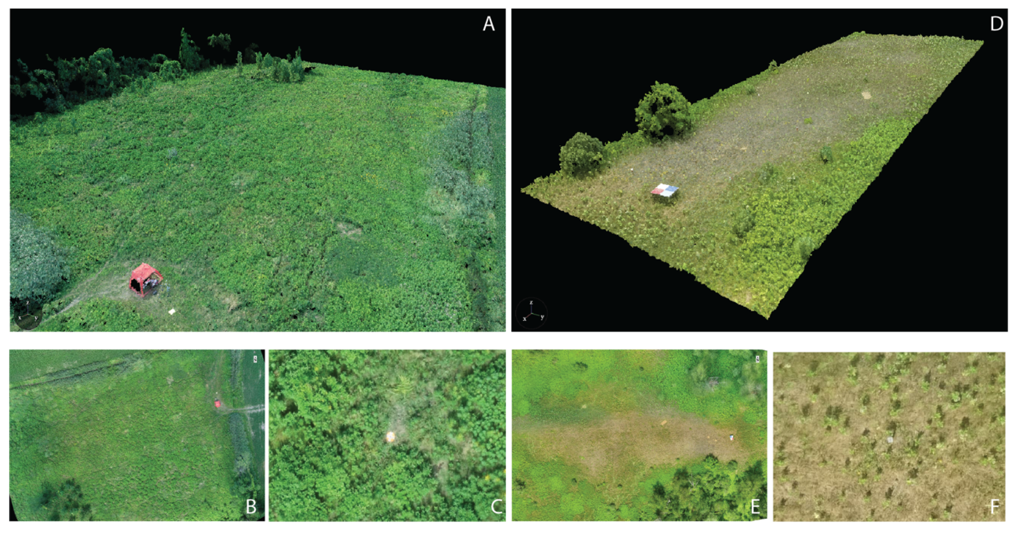
2.1. Study Sites

This study was carried out over a three-year period at three mid-latitude sites in Eastern Canada (shown in Figure 2): (1) a 2.8 ha field of herbaceous vegetation next to the Mer Bleue peatland (MB), near Ottawa, Ontario (Figure 2A); (2) an abandoned 3.7 ha agricultural field on île Grosbois (IGB), near Montreal, Quebec (Figure 2B); (3) a 1.5 ha agricultural field in Rigaud, Quebec (Figure 2C). As a means to introduce checkpoints to validate the horizontal and vertical accuracies of the SfM and SfM-MVS products, 70 cm tall wooden posts were placed in the field at MB. Each post had a 10 cm wide metal plate affixed to the top. The plates were painted matte grey and marked with an “X” in the center using contrasting (black and white) tape. These posts were installed for multi-year use at the site (Figure 2D). At the two other sites, checkpoints consisted of circular plastic orange bucket lids (30.5 cm diameter and 23.5 cm diameter) marked with an “X” in contrasting tape that were placed flat on the ground randomly before each flight (Figure 2E). All three study sites have relatively low topographic variability comprised of the variable herbaceous vegetation height at MB and IGB and the soil separating the furrows in the plowed field (Rigaud). For all flights, the weather was sunny with few clouds and little wind.

2.2. UASs and Camera Systems Tested

We tested fourteen UASs ranging in weight from 430 g to 14 kg (Table 1 and Table 2). Flights were conducted at 30–45 m above ground level (AGL) nominally, with orthogonal flight lines. The Phantom 4 RTK (P4RTK), the Matrice 600 Pro RTK (M600P), and Matrice 210-RTK (M210-RTK) required an external base station to function in RTK flight mode. Flight line spacing and camera triggering were optimized for each system by the flight controller software while maintaining 80% frontlap and sidelap coverage. Photographs were collected at nadir with the exception of the Mavic Air for which the maximum allowable angle by the flight controller software was –80°. All onboard cameras were triggered directly by the UAS. Shutter speed, ISO, aperture and exposure compensation were automatically set by the on-board cameras without user intervention. The onboard cameras were also set to autofocus mode.
For the M600, the digital single-lens reflex (DSLR) camera was mounted on a Ronin MX gimbal (DJI, Shenzhen China) for stabilization and orientation. Two configurations were evaluated: (1) PPK mode where geotagging was achieved via an M+ RTK GNSS module (Emlid, St Petersburg, Russia) to record the position and altitude and a PocketWizard MultiMax II intervalometer (LPA Design, South Burlington, VT, USA) to trigger the camera at 2-second intervals; (2) in stand-alone mode, the DSLR was also triggered by the intervalometer but geotagging was automated with a Canon GP-E2 GPS receiver connected to the DLSR’s hot shoe. In all cases, the DLSR was operated in “programmed auto” mode, in which the aperture and shutter speed are automatically set by the camera but the user has control of the ISO and exposure compensation. The ISO was set to 800 with no exposure compensation. The lens was set to autofocus, using all of the available points of the camera’s autofocus sensor.
The P4RTK received RTK corrections from the Can-Net CORS network via a virtual reference station (VRS) mountpoint utilizing both GPS and GLONASS constellations. All P4RTK photographs were captured in the fixed status for maximum geolocation accuracy. Three types of geotagging were implemented for the M600P DSLR photographs collected in PPK mode. First, with the “local base” configuration (PPKLB) a base station dedicated to collecting GNSS data for the photographs was set up. For this, we used an RS+ single-band receiver (Emlid, St Petersburg, Russia). Second, for the local base configuration with the added NTRIP correction (Networked Transport of Radio Technical Commission for Maritime Services (RTCM) via Internet Protocol), PPKLB-NTRIP, the RS+ base station received the incoming corrections from the SmartNet North America NTRIP casting service on an RTCM3-iMAX (individualized master-auxiliary) mount point utilizing both GPS and GLONASS constellations. These corrections were transmitted to the M+ receiver onboard over LoRA (long-range) 915 MHz radio. Lastly, for the PPK configuration with a commercial base station, PPKCB, the SmartNet North America station in Vaudreuil-Dorion (Station QCVD—16 km baseline) was used in post-processing.
All photographs (from all UASs) were acquired as jpgs except for the DSLR, which acquired photographs in Canon RAW (.CR2) format. These were subsequently converted to large jpg in Adobe Lightroom® with minimal compression for analysis.

2.3. Photograph Geotagging

The non-RTK/PPK systems automatically geotag the acquired photographs with the horizontal and vertical position of the UAS time-synchronized to the onboard GNSS receiver (and camera attitude) with the exception of the Mavic Air that writes the horizontal position to the Exif data, but for altitude only records the barometer measurement (height above the take off point). Therefore, for the Mavic Air, elevation (HAE) was manually calculated based on the flight altitude and the elevation of the take-off point and added to the Exif. The P4RTK automatically geotagged photographs with the incoming RTK corrections applied. For all UASs, in addition to the geotagged position, the camera roll, pitch and yaw at the time of frame acquisition was also written into the Exif.
For the DSLR photographs with positions determined via PPKCB, PPKLB and PPKLB-NTRIP, the horizontal coordinates and altitude needed to be calculated in post-processing. The open-source RTKLib software [65] was used to calculate the geotag of each DSLR photograph. For the PPKLB-NTRIP configuration, the geotags were calculated with and without precise clock and ephemeris data downloaded from the Natural Resources Canada’s Canadian Geodetic Survey. For each of the DSLR PPK configurations, a lever arm correction was also applied. The precise DSLR attitude on the Ronin MX at the time of frame acquisition is not recorded.
For the photographs geotagged with the onboard GNSS receivers (no RTK or PPK correction), the altitude tags were discarded due to the large errors recorded in the Exif data by each system (>10 m in some cases). The altitude tags were manually recalculated from the barometer measurements of altitude above the take off point (m ASL or HAE) added to the known ground elevation. The accuracy of the barometer measurements had previously been assessed to be ±10 cm [22]. Because the GP-E2 does not have a barometer the correct altitude was determined from the flight logs and a lever arm correction. For the P4RTK the lever arm correction is automatically taken into account in the positions recorded in the Exif.

2.4. Checkpoint Position Measurement

The targets used as checkpoints were measured after every flight. On August 15, 2019, ten checkpoints were measured using a Trimble Catalyst GNSS/RTK receiver with corrections obtained using the Can-Net VRS network. Only points with a fixed status were considered in the analyses. At MB and Rigaud, the RS+ with incoming corrections from the SmartNet North America NTRIP service was used after all flights (fifteen checkpoints). The accuracy of the RS+ with the incoming NTRIP correction was previously verified in comparison to the location of the Natural Resources Canada High Precision 3D Geodetic Passive Control Network station 95K0003 in Dorval, Quebec. The error in the computed position of the station by the RS+ was determined to be 0.6 cm (X), 2.7 cm (Y) and 5.1 cm (Z). For the Trimble Catalyst, the accuracy was assessed to be <2.5 cm (X and Y) and <3 cm (Z) as reported by the system. The dual-frequency Trimble Catalyst was considerably faster at achieving a fixed position than the RS+ (<10 sec vs up to 15 min).

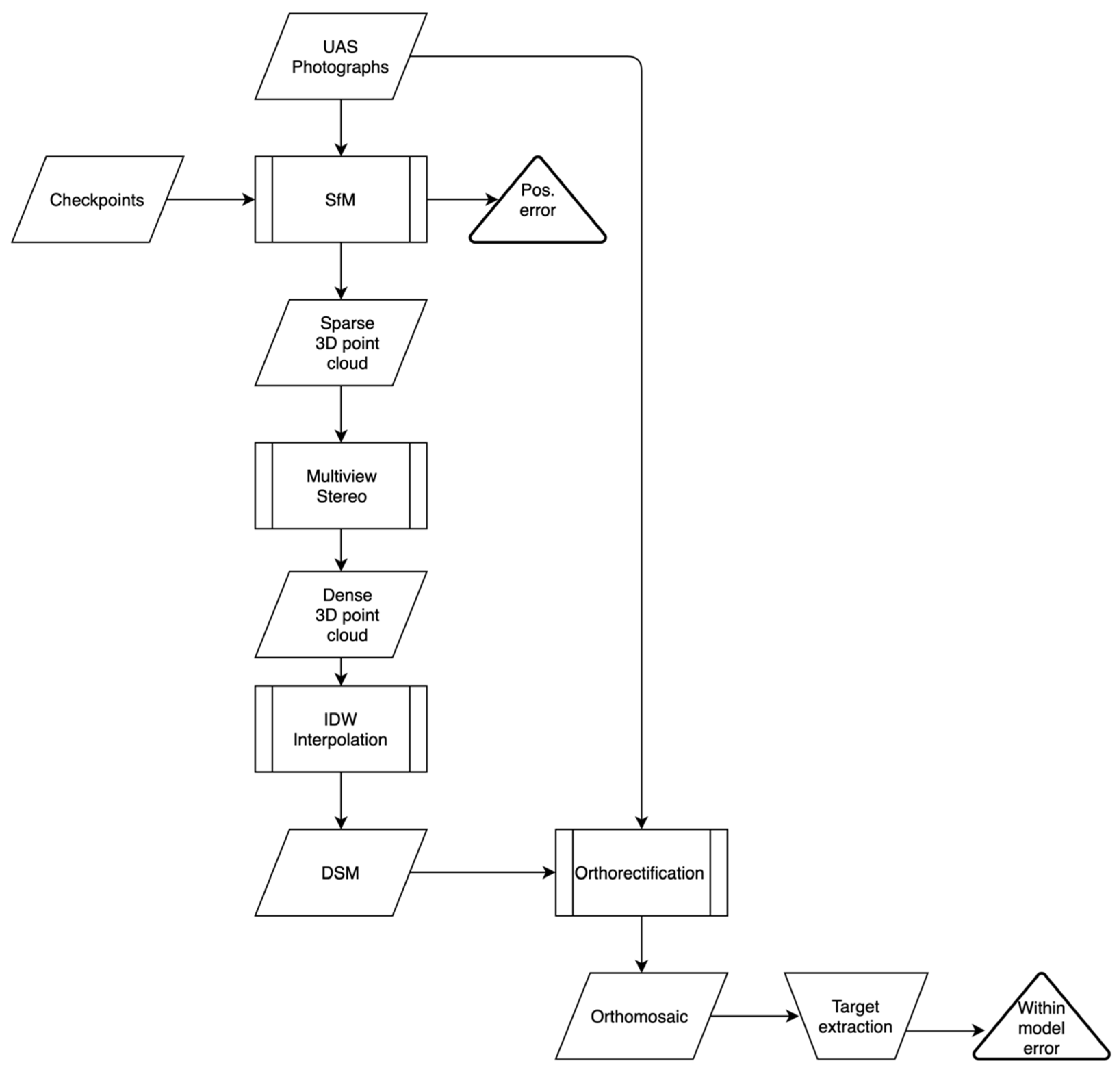
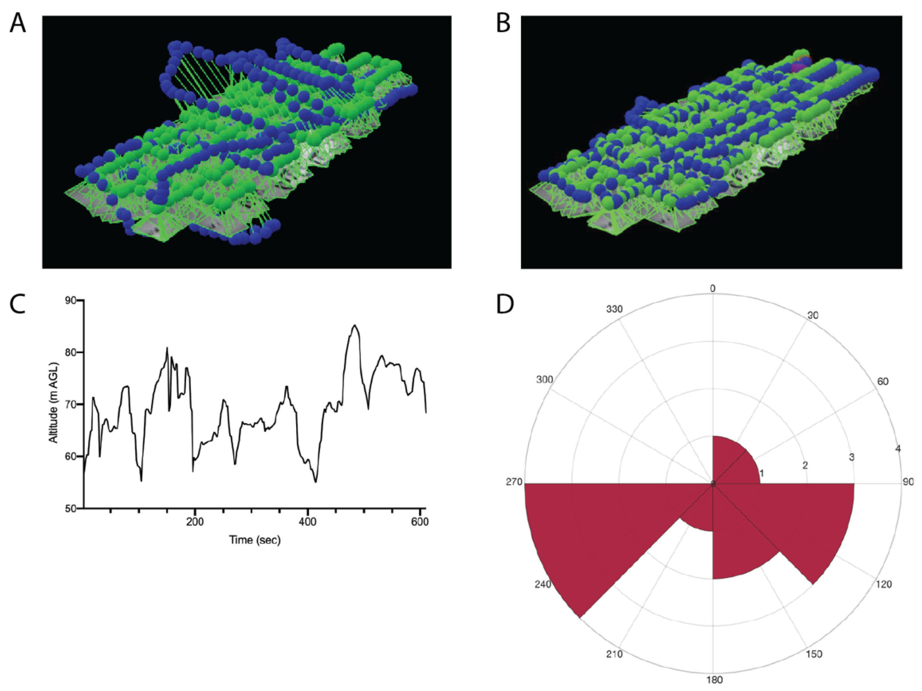
2.5. Structure from Motion–Multiview Stereo (SfM-MVS) Processing

An SfM-MVS workflow (Figure 4) was carried out in Pix4D Mapper (Pix4D S.A, Prilly, Switzerland) to reconstruct the study areas after each flight. The two main products of interest in our study were the sparse 3D point cloud because during its generation the positional accuracy of the model is computed in relation to the checkpoints, and the orthomosaic from which the within-model horizontal distances were computed. For photographs with camera orientation information in the Exif (i.e., all except the DSLR), Pix4D converts these to Omega, Phi and Kappa angles (rotation between the image coordinate system and a projected coordinate system) [66,67]. Key components of Pix4D’s workflow are the calibration and optimization during which an automatic aerial triangulation, bundle block adjustment, and camera self-calibration steps are carried out (see [68] for details). Pix4D generates the sparse 3D point cloud through a modified scale-invariant feature transform (SIFT) algorithm [69,70]. Following the generation of this initial 3D point cloud, an MVS photogrammetry algorithm densifies the point cloud [71] (Figure 4). Subsequently, a raster DSM is created through an inverse distance weighting (IDW) interpolation of the dense 3D point cloud. The DSM includes objects such as trees and buildings as part of the model (as opposed to a digital terrain model (DTM), which represents the bare earth elevation). The DSM and the input photographs are used to create an orthomosaic without perspective distortion.

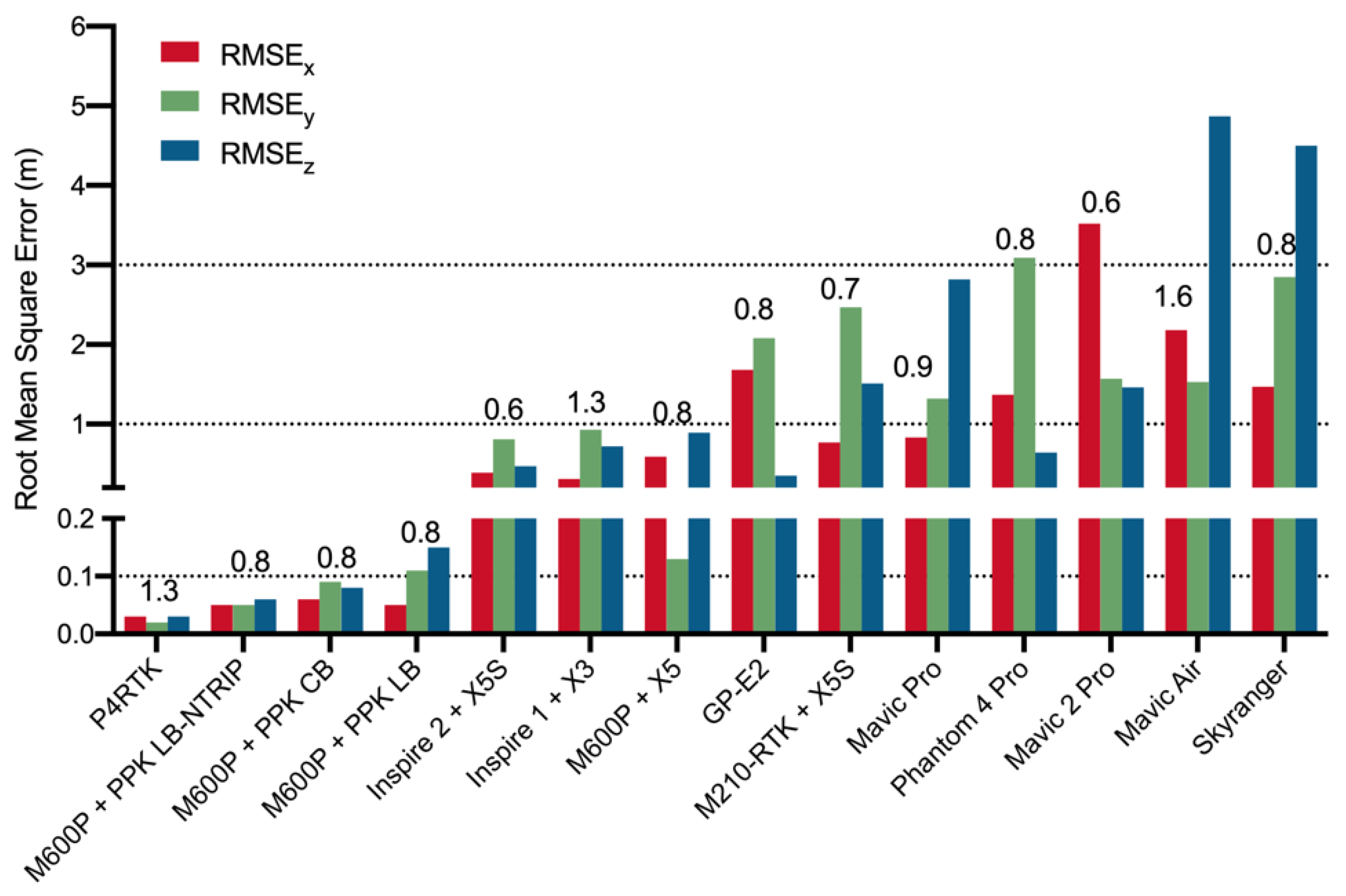
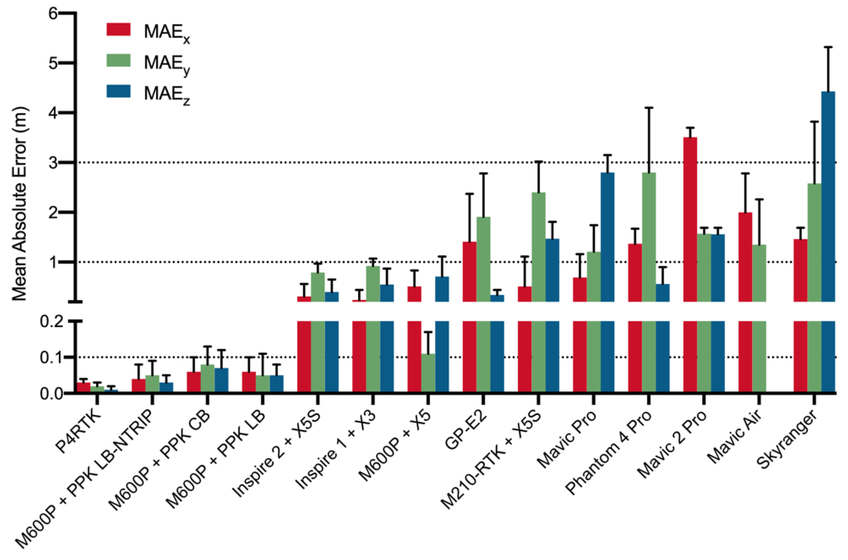
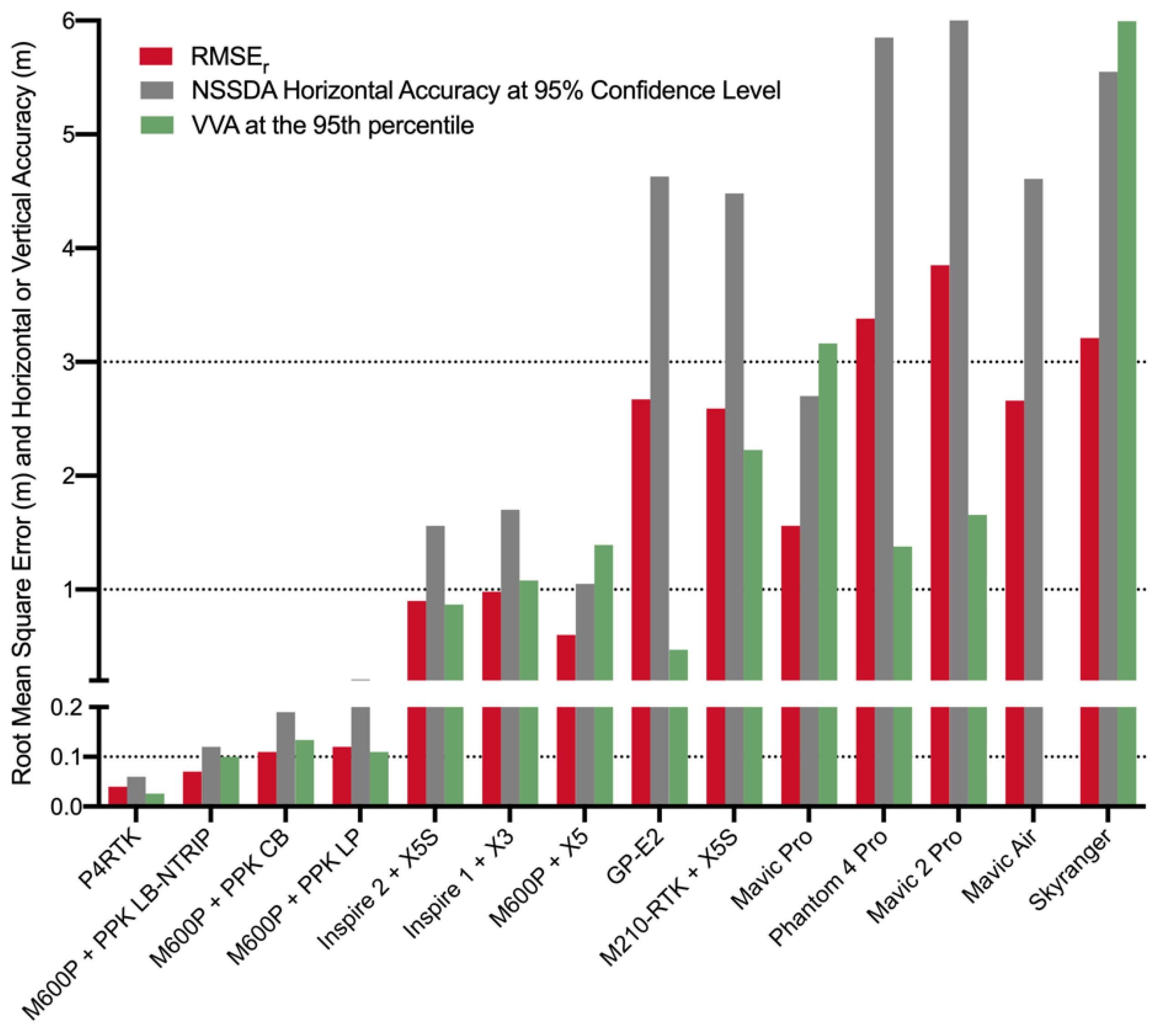
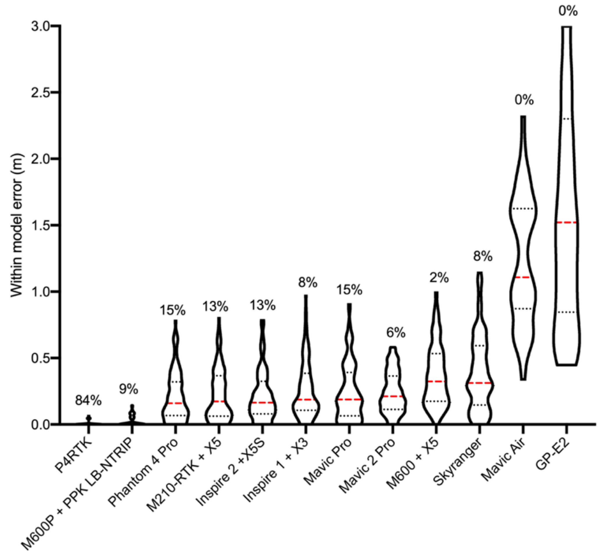
2.6. Model Accuracy Assessment

Horizontal (x and y) and vertical (z) positional accuracies were determined for the SfM models from the coordinates of the checkpoints within Pix4D (Figure 4). From the reported values of RMSEx and RMSEy, the horizontal linear RMSE in the radial direction (includes both x- and y-coordinate errors, RMSEr) and National Standard for Spatial Data Accuracy (NSSDA) horizontal accuracy at a 95% confidence level were computed according to Equations 1 and 2 following [61]. Because the vertical error in vegetated terrain (z-component) typically does not follow a normal distribution, the vegetated vertical accuracy (VVA) at the 95th percentile is calculated following [61] (and discussed rather than RMSEz).
R M S E r = R M S E x 2 + R M S E y 2
H o r i z o n t a l   a c c u r a c y   a t   95 %   c o n f i d e n c e   l e v e l = 1.7308 × R M S E r
where RMSEx is the horizontal linear RMSE in the easting and RMSEy is the horizontal linear RMSE in the northing. In the computation of RMSEx and RMSEy the NSSDA assumes that the errors are random errors that follow a normal distribution. We computed the D’Agostino–Pearson omnibus k2 test for normality on Δx and Δy. This tests against the alternatives of skewed and/or kurtic distributions. Due to the smaller than recommended sample size for checkpoints [61], the significance of RMSEr and the VVA at the 95th percentile should be treated with caution.
The within-model horizontal accuracy was determined by comparing the distances between all pairs of checkpoints from the orthomosaic and from the field measured coordinates. The locations of the targets in the orthomosaics were manually located, and the coordinates extracted with ArcMap 10.7. For the distance calculations between pairs of checkpoints, we took into consideration standard error propagation of the uncertainty in the coordinates of the checkpoints as determined on the ground, as well as user uncertainty locating the exact center of checkpoints in the orthomosaics. User uncertainty in digitization was estimated at a maximum of 2 pixels in x and y. For the uncertainties in the ground GPS measurements, the values described in Section 2.3 were used. The error propagation to determine the uncertainty in the distance measurements was done by calculating the partial derivatives of the distance between two points with respect to both the x and y coordinates, multiplication with the uncertainty of those two variables, and addition of those terms in quadrature (Equations 3 and 4).
D = f ( x i , x j )
δ D = ( D x i × x i ) 2 + ( D x j × x j ) 2
where D is the distance between the location of the two checkpoints (xi and xj) and δD is the uncertainty in the distance calculation.

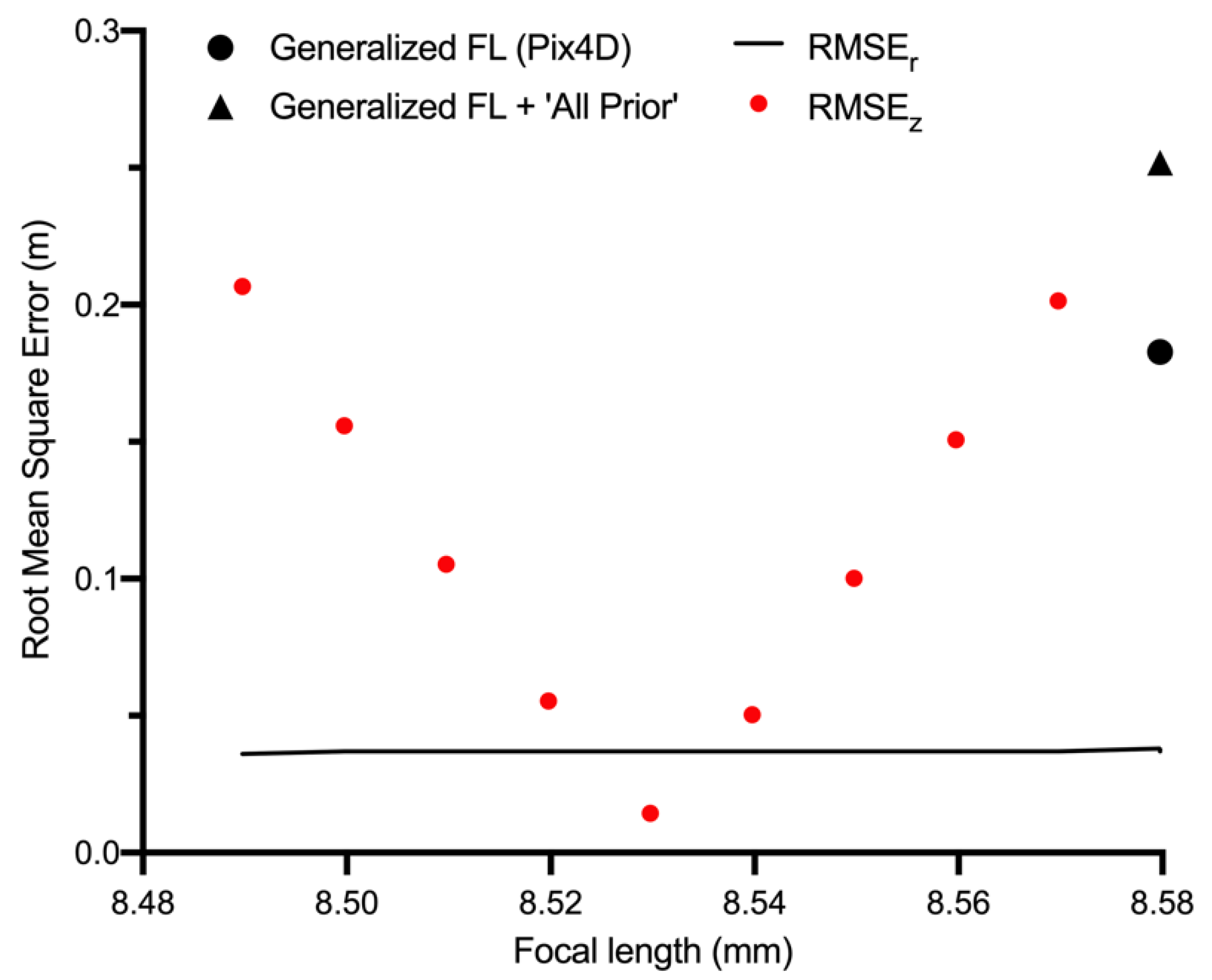
2.7. Camera Focal Length Considerations for the Phantom 4 RTK

For the P4RTK, we initially followed Pix4D’s recommended workflow [72], which included applying the built-in optimized camera parameters. For greatest accuracy, all photograph and checkpoint coordinates were first converted to UTM (zone 18N) coordinates and ellipsoidal heights with NAD83(CSRS) 2010 epoch as the reference frame, using Natural Resources Canada’s TRX software [73]. The same reference frame was used for the outputs. The TRX software also allows the user to set the GPS epoch correctly (i.e., provinces adopted different epochs, see [74]).
Initial results for the P4RTK using this recommended workflow yielded low RMSEx, RMSEy, RMSEr (2–4 cm), but an 18 cm RMSEz (Table 3, Figure 5). Setting the initial camera parameters from “All” to “All prior”, as recommended by Pix4D, actually made results worse (Table 3, second row). The “All prior” setting forces the optimal internal parameters (focal length, coordinates of principal point, radial distortion parameters and tangential distortion parameters), to be close to the initial values from the camera database. In contrast, “All” optimizes these parameters starting from the initial values in the database with subsequent recalculation. The values are recalculated based on the calibrated photographs in the dataset [68]. We manually decreased the focal length parameter in the camera description by 0.01 mm increments, keeping the “All prior” setting to fix the new focal length. The lowest RMSEz (1.4 cm; Table 3, Figure 5) was obtained by reducing the default focal length from 8.58 mm to 8.53 mm, after which the vertical accuracy gradually worsened (Table 3, Figure 5). Horizontal accuracy (RMSEx, RMSEy and RMSEr) was largely unaffected by the focal length. We used the optimized camera parameters from the best model for all other analyses, using the “All prior” initial camera parameter calibration setting.

3. Results

Summary statistics comprised of the RMSE(x,y,z,r) and mean absolute error (MAEx,y,z) are shown in Figure 6, Figure 7 and Figure 8 to illustrate Δx, Δy and Δz between the SfM model derived checkpoint locations and those measured in situ. Both MAE and RMSE measure the average magnitude of the positional errors, however, the RMSE is more sensitive to large errors (outliers). For this reason, and because RMSEz is not expected to follow a normal distribution in vegetated terrain, the VVA at the 95th percentile (Figure 8) is examined to quantify the positional accuracy in elevation.
As expected, the UAS with RTK or PPK geotagged photographs produced models with the lowest positional errors (RMSE, MAE and VVA). These were also the most accurate systems for the within-model measurements of distances between checkpoints (Figure 9). The P4RTK, a system specifically designed for enterprise SfM-MVS photogrammetry, includes an incoming NTRIP correction to its base station and directly applies RTK corrections to the geotags of the photographs. Both the positional error (RMSEr: 4 cm, MAEz: 1 cm, VVA: 3 cm) and within-model error (μ = 0.8 ± 2 cm) of this system are analogous to the low errors achieved by various UASs as reported in the literature with GCPs included in the processing (see summary by [59]) (Figure 10A–C). It is also the system with the highest percentage (84%) of within-model distance calculation errors that were less than the uncertainty of the measurements (Figure 9). In order to achieve the high vertical accuracy, an important consideration for the P4RTK is the calculation of the specific focal length of the lens unique to the system being used (Table 3, Figure 5). The generalized camera model focal length within Pix4D (8.58 mm) resulted in unreasonably high vertical errors (18–25 cm) for our particular camera. It is possible that other users with camera focal lengths closer to the default Pix4D values could get high vertical accuracies out of the box.
The UAS with the second-lowest positional and within-model errors (M600P + PPKLB-NTRIP) overcomes the lack of onboard generated geotags through third-party hardware and software resulting in a 7 cm RMSEr, 3 cm MAEz, 10 cm VVA and low within model error (μ = 3 +/− 4 cm) (Figure 6, Figure 7, Figure 8 and Figure 9). While this system had a low percentage of within model distance errors less than the uncertainty of the measurements (9%), the errors were close to the uncertainty estimates (Figure 9). The same system performed slightly worse (higher error) with PPKCB and PPKLB (Figure 6, Figure 7 and Figure 8). Negligible differences were seen by using the fast versus precise clock and ephemeris data (PPKLB-NTRIP).
The remaining systems relying on onboard GNSS geotagging resulted in positional errors ranging from an average RMSEr of 0.60 m (M600P + X5S) to >3 m (SkyRanger, Mavic 2 Pro and Phantom 4 Pro) (Figure 6, Figure 7 and Figure 8). It is important to note that for the three UASs with RMSEr > 3 m, there is a substantial difference in RMSEx vs RMSEy (and MAEx versus MAEy) (Figure 6 and Figure 7) resulting in the larger values of RMSEr. For operational use without GCPs for these UASs, results suggest further investigation would be warranted to determine, if possible, the reason for the larger error in one direction. Overall, the non-RTK/PPK systems were consistent in the within-model horizontal distance measurement errors (μ = 0.21–0.26 m) except for the SkyRanger (μ = 0.39 +/− 0.28 m) and Mavic Air (μ= 1.2 +/− 0.48 m) (Figure 9). All non-RTK/PPK systems have a lower within-model distance error compared to the positional error (RMSEx,y,r or MAEx,y) (Figure 6, Figure 7, Figure 8 and Figure 9).
The distributions of the within-model horizontal measurement errors presented as violin plots (Figure 9) are important to consider because this provides an indication of the homogeneity of the spatial errors throughout the SfM-MVS orthomosaics. For non PPK/RTK systems the broad range of within-model error values indicates that errors are spatially inconsistent. The greatest range can be seen for the GP-E2 (0.45–3.9 m, μ = 1.67). The original geotags of this GNSS module recorded the largest vertical errors and erratic horizontal positioning (Figure 11A,C). Following the replacement of the original altitude tags in the Exif by the altitude (AGL) recorded in the flight logs with a lever arm correction applied (Figure 11B), the SfM model still resulted in within-model errors with an inconsistent and variable (up to ~90°) orientation (Figure 11D). On the western side of the model, the displacement between known checkpoints and those in the orthomosaic are mainly E–W oriented, while on the eastern side they are predominantly N–S. The large discrepancies in the original altitude tags (Figure 11C) as well as horizontal position, indicates that the GP-E2 is inaccurate for SfM or SfM-MVS reconstructions. It has been previously shown that the M600P computes a GNSS altitude of +/− 1 m during flight. Furthermore, the altitude computed from each of the three A3 Pro modules can vary up to ~2 m between modules [22]. However, with RTK enabled in the flight controller (as was done here), the altitude difference recorded between the three modules is reduced to <1 cm and overall the altitude varies by 5–10 cm during flight [22]. This can also be seen in Figure 11A,B in the position of the optimized photograph locations in comparison to the original geotags.
The other UASs for which processing needed to be modified was the Mavic 2 Pro with the integrated Hasselblad L1D-2C camera. The standard pipeline for processing that allows Pix4D to optimize the camera internal parameters and recalculate/optimize the position and orientation of the photographs resulted in a domed SfM point cloud (radial distortion) (Figure 12A). By setting the initial camera parameters from “All” to “All prior” and selecting the “Accurate Geolocation and Orientation” option, the distortion was removed (Figure 12B). The “All prior” option alone did not remove the deformation. While this alternate pipeline is generally recommended for RTK/PPK solutions that also have accurate IMU information (≤3°) it can improve SfM products from other systems as well as seen here.
The lower positional and within-model accuracy for the Mavic Air (Figure 6, Figure 7, Figure 8 and Figure 9, Figure 13) was expected because it is a consumer-grade system that was not developed for photogrammetry purposes or precise flight controls as would be required by professional or enterprise systems. The high positional error (RMSE and MAE) and low within-model accuracy of the Skyranger were unexpected given it is an enterprise UAS (Figure 6, Figure 7, Figure 8 and Figure 9, Figure 10d–f, Figure 13).
In general, we found that the cost of the system is only weakly related to the accuracy of the models generated by the different systems (Figure 13). The two most accurate systems (P4RTK and M600P + PPKLB-NTRIP) fall into the second-highest cost category (US$5000–$15,000) but the most expensive system tested (SkyRanger, >US$100,000) has both low positional accuracy (high RMSEr and MAE) and high horizontal within-model measurement error (μ = 39 +/− 28 cm). The majority of the non-RTK/PPK systems, which ranged in price at the time of purchase from US$2000–$15,000, perform similarly in terms of both positional accuracy and within-model accuracy.
Based on the 2015 American Society for Photogrammetry and Remote Sensing (ASPRS) positional accuracy standards for digital geospatial data [61], only the P4RTK and the M600P + PPKLB-NTRIP SfM-MVS products could be used without GCPs for projects requiring high spatial accuracy (Figure 14). The accuracy requirements of SfM or SfM-MVS products (RMSEAT) to be used for elevation data and/or planimetric data (orthomosaic) production or analysis is calculated as (Equation (5)) [61]:
R M S E A T   = 1 2 × R M S E M a p , D E M
where RMSEAT is the RMSEx,y,z the SfM-MVS product must meet, and RMSMap,DEM is the project accuracy requirement. For example, a forestry inventory requirement of RMSEMap of 2 m would require an SfM-MVS orthoimage with an RMSEAT of no larger than 1 m. RMSEAT is shown as the finest RMSEMap,DEM for which the UAS products generated here could be used (Figure 14).
Figure 14 also illustrates that without GCPs, six UASs could be used to support manned aircraft such as airborne hyperspectral imagery or high spatial resolution satellite generated (e.g., Planet Dove, Pleiades). The remaining six UASs with the largest RMSEAT could be used to support projects with moderate resolution satellite data products (e.g., Sentinel-2, Landsat).

4. Discussion

We found that eight of the fourteen of UASs tested can achieve relatively high positional (RMSEr < 2 m) and within-model accuracies (<0.5 m) for SfM and SfM+MVS models without GCPs. A clear distinction in horizontal and vertical accuracy was whether the UAS photographs were tagged with a PPK/RTK solution or not, regardless of the flight controller’s use of RTK for navigation. Similar to other studies (e.g., [75,76]) a PPK/RTK GNSS solution resulted in low positional errors without GCPs. Depending on the purpose of the data collections (e.g., animal counts), users may not need high positional accuracy to real-world coordinates, and therefore, the within-model measurement error may be more important. Twelve of the UASs had average within-model errors of <0.4 m, four systems (the M600P PPK configurations and the P4RTK) each had an average error <3 cm, and one (P4RTK) had an average linear within-model error of 0.8 cm with a range of 0–6 cm. In this case, 0 refers to errors less than the uncertainty of the measurements.
As this work shows, in order to achieve the low vertical positional error with the P4RTK, the user must determine the camera-specific focal length (one of the leading internal camera parameters); a calculation that is relatively easy to do. This is likely due to minute differences in lens element distortions and other internal camera parameters between individual units. As such, it is likely that the out-of-the-box generalized focal length will not result in the advertised survey-grade accuracy for all units. It is also the only UAS we tested where the integrated camera tagged the photographs with a dual-frequency GNSS position calculation using both GPS and GLONASS. Additional frequencies provide for better signal reception within close proximity to obstacles such as trees and buildings and reduce ionospheric error in the position calculation. Generally, dual-frequency systems also achieve a “fixed” GNSS solution considerably faster than single-band systems and are more accurate. While not tested here, it is also likely that the D-RTK2 base station of the P4RTK (can utilize GPS L1, L2, L5, GLONASS F1 and F2, Galileo E1, E5A and E5B, and BEIDOU B1, B2 and B3) can achieve a more precise position calculation even without an incoming correction than the earlier generation D-RTK base station of the M600P and M210-RTK (GPS L1 and L2, GLONASS F1 and F2). However, an incoming correction is important to achieve the highest positional accuracy. Contrary to expectations, the model from the Inspire 1, which uses a single frequency GNSS receiver that also only receives GPS L1 with no GLONASS support had lower positional and within-model errors than six other UASs that also support GLONASS F1 (Table 1, Figure 13) indicating that under the right conditions (i.e., good GNSS geometry, no obstacles and a low planetary k index) it is possible to achieve acceptable results using a single GNSS constellation.
Not all “RTK” systems geotag the photographs with the RTK corrected coordinates (e.g., M210-RTK, M600P + X5). In these systems, RTK is only used for accurate navigation. Newer systems such as the M210-RTK v2 (not tested here) and the P4RTK include the RTK corrections in the geotags. As such, users need to be aware of the characteristics of the systems they purchase. In order to accurately geotag the photographs from the M600P with the DSLR camera, third-party hardware and software needed to be incorporated into the setup with a PPK workflow. While this did result in high accuracy, these configurations (PPKLB, PPKCB, PPKLB-NTRIP) are considerably more complicated to operate with multiple potential points of failure (i.e., hardware from multiple manufacturers and human error in setup/operation) than integrated systems such as the P4RTK. These DSLR configurations also require precise lever arm measurements to correct for the distance from the GNSS antenna to the film plane (detector array) on camera when the geotags are calculated in post-processing. For example, for the DLSR mounted on the Ronin MX gimbal on the M600P, the vertical distance between the GNSS antenna of the M+ and the DSLR’s film plane was –50.2 cm. These measurements should be taken every time the DSLR is installed and balanced on the gimbal. Novel SfM-MVS object reconstructions of the airframe, as shown by [77], allow for digital preservation of the system and precise measurements post-flight.
A common aspect of all non-RTK/PPK systems was that the altitude recorded in the Exif is of very low accuracy and should not be used for SfM-MVS if GCPs are not included in the processing pipeline. We recommend that users replace these values by ones they calculate themselves from the barometer value added to the ground elevation (m AGL or m HAE). Until more accurate GNSS altitudes are possible from small non-RTK/PPK UASs, the original values (errors in altitude up to >10 m) recorded in the Exif are unreliable (e.g., Figure 11A). Furthermore, manufacturer documentation related to the coordinate systems (horizontal and vertical) generally lacks critical details, especially for the vertical component, which would allow for more precise transformations between datasets. In the case of RTK/PPK systems, the coordinate systems are readily determined because they correspond to those of the base station, and therefore, precise transformations can be carried out.
The relatively high errors of the Mavic 2 Pro (compared to the Mavic Pro) and the SkyRanger were unexpected. Despite having a superior camera in comparison to its predecessors, the Mavic 2 Pro is the system with third-largest RMSEr (Figure 8), and also the one with the deformation of the SfM sparse point cloud without additional consideration for the processing steps (Figure 12). In contrast to its predecessors (Mavic Pro and Mavic Air), this system integrates a 1 inch L1D-2C camera. As this relatively new UAS was not designed specifically for mapping it may take additional versions of firmware upgrades to improve the positional information in the Exif of the photographs and characterization of the camera internal and external parameters. The domed output is indicative of incorrect camera model parameters [78]. Changing the calibration to “All prior” with “Accurate Geolocation and Orientation” removes the deformation error by not attempting to recalculate camera model characteristics from the photographs. In landscapes such as our study areas that are topographically flat relative to the flight altitude, optimization can introduce errors where the distance to the surface is wrongly calculated. Ideally, there should be a low correlation between the internal camera parameters. However, some correlation is unavoidable in flat terrain [79]. Correlation among the leading parameters (i.e., focal length (F) and the x, y coordinates of the principal point) result in errors in the SfM reconstruction. In the case of the Mavic 2 Pro, high correlations were seen in the reconstruction with the domed output (Figure 15).
A potential source of error not addressed here but requiring further study is the impact on SfM and SfM-MVS products of the radiometric degradation of from lossy compressed files with low bit depth (i.e., jpg) rather than lossless TIFs generated from RAW files captured by the sensor. Of the cameras tested, only the DSLR was capable of collecting photographs in RAW while mapping, the others all save to jpg. The onboard processors of the UAS lack the write speed to save RAW images at the rate they are taken for photogrammetry. It is well known that manufacturers (hardware and/or software) implement proprietary jpg engines, which apply varying degrees of processing and compression; therefore, each set of photographs from the UAS underwent different jpg generation pipelines within the cameras, or within Adobe Lightroom® for the DSLR. A jpg with 8 bits can represent a maximum of 256 digital numbers (DN) per color channel. A 14-bit sensor such as used by the DSLR can represent 16,384 DN per channel when the file is saved in RAW (or exported as a lossless tiff). The total theoretical color depth of an 8-bit photograph is 16,777,216 colors in comparison to 4.398 × 10¹² for a 14-bit RAW DSLR photograph. In one example, exporting the M600P + PPKLB-NTRIP photographs with twice the jpg compression (100% jpg quality versus 50%) resulted in lower positional accuracy of the SfM model: RSMEx increase of 1 cm, RMSEy increase of 2 cm and an RMSEz increase of 2.9 cm. A similar decrease in accuracy was found by [80] in a comparison between SfM reconstructions from RAW photographs versus jpg. A comparison of the number of pixels whose DN was different between the 100% and 50% jpg quality indicated that only 55% of the pixels retained their DN with the greater compression. The remainder changed by up to 52 DN. The effects of compression on a photograph are scene dependent, and therefore these values are simply provided as an example that the well-known degradation from lossy compression (e.g., jpg) does matter for SfM and should be minimized when possible.
Acquiring photographs in RAW format requires computational speed to ensure the files are written to the media at a rate faster than they are taken by the camera. The write speed of the files is determined by both the onboard processor of the camera, and the type of media used. Because the Inspire 2 was designed for cinematography (internal CineCore processor capable of 6K RAW video recording) and has the option to write directly to a high-speed SSD instead of a micro SD card, it is plausible that it could in the future, with changes to its firmware, be used to collect photographs in RAW for mapping purposes. RAW files are more flexible to allow for adjustments to produce uniform (in color, saturation and exposure) photographs needed for improving the overall quality and visual appeal of SfM-MVS models. Potentially, the new lossy compressed format, HEIF, which supports higher bit depth than jpg while retaining a small file size may be a suitable compromise between image quality and write speed limitations.
Additional aspects requiring further study include an investigation into the impact of the pixel size, sensor modulation transfer function (MTF) and signal to noise ratio on the accuracy of SfM-MVS products. While we found a correlation of r = −0.55 between pixel size (Table 2) and RMSEr (Figure 8) it was not significant (α = 0.05). However, we believe that for non-RTK/PPK systems the sensor size (and, independently, pixel size) is more strongly related to the grade of the system (e.g., consumer vs professional or enterprise). In addition to a smaller sensor, with smaller pixels, a consumer-grade UAS, such as the Mavic Air or Mavic Pro also has a lower accuracy GNSS modules and/or algorithms for the computation of their position. In terms of the sensor and pixel sizes, the SkyRanger is an outlier because it uses a back-illuminated sensor. In contrast to conventional front-illuminated sensors, the wiring, which reduces the number of photons being recorded, is placed under the photodiode substrate allowing for greater sensitivity and higher resolution (more and smaller pixels) on smaller sensors. Ref. [81] found that for small sensors, the light sensitivity of pixels with less than 3.2 µm pitch decreases with further pixel size reduction. In an examination of the tradeoffs between spatial resolution (i.e., more smaller pixels) and noise, they determined a theoretical maximum image information capacity based on the signal to noise ratio and MTF of individual pixels as 1.45 µm. Real-world testing of sensors from different manufacturers revealed, however, that variations in quality between manufacturers were greater than the effect of differences in pixel pitch. With the exception of the SkyRanger’s camera (pixel size of 0.99 µm), we found that all UASs tested here with a small sensor (1/2.3”) have a pixel size close to the theoretical maximum image information capacity: Mavic Air = 1.50 µm, Mavic Pro = 1.57 µm, X3 = 1.58 µm (Table 2). All UAS cameras tested here with a 1” sensor have a pixel size of 2.35 µm. Only the M4/3 and full-frame sensors surpass 3.2 µm in pixel size. It is further important to remember that despite generic characterizations of sensors in terms of mega-pixels or image size, due to the Bayer color filter pattern used by the majority of sensors in photographic cameras (including all cameras tested here), the capture ratio, and native resolution of the green channel is twice that of the red and blue channels [80].
Also, rather than focusing on smaller/more compact sensors, the latest models of mirrorless cameras and larger flange diameter lenses may improve individual photo quality due to their higher light sensitivity and increased sharpness and larger image size. It is however uncertain how much the increase in overall sharpness and dynamic range may improve the accuracy and overall details of the SfM-MVS products. Early issues with short battery life seem to have been fixed in the most recent models. Medium format and high megapixel 35 mm format cameras may not substantially improve the SfM-MVS model accuracy, due to oversampling at low altitude compared to the accuracy of onboard GNSS or even RTK/PPK solutions. These systems would likely be of greater benefit for higher altitude flight (e.g., >150 m), but this also increases atmospheric effects (e.g., haze).
Importantly, this study was conducted at vegetated sites with low topographic relief. Further analysis is warranted over sites with highly variable terrain and a range of materials, natural and manmade (e.g., monuments and buildings) as well as aquatic systems to fully characterize the systems. Comparison with georeferenced terrestrial laser scanning (TSL) products of these more complex landscapes would further allow for quantifying the accuracy of geometries. We anticipate differences in RMSEr and non-vegetated accuracy (NVA for impermeable surfaces) in comparison to our results.
All our SfM reconstructions were carried out with the same software. As has been shown by [25,82,83], results can vary based on the software due to differences in the processing algorithms. Nevertheless, we expect the general pattern of accuracy ranges for the various UASs to be consistent across software implementations even if the absolute values for the accuracies may differ.
Lastly, for the use of RTK/PPK UASs in remote areas the impact of calculating the base station position from a precise point positioning (PPP) solution should be investigated. Due to the general stated accuracies of PPP of 10–30 cm, the SfM-MVS products would achieve slightly lower accuracies under a best-case scenario.

5. Conclusions

Because for many UAS 3D landscape reconstruction applications, the use of GCPs is not feasible, our study assessed the horizontal and vertical accuracies (positional and within-model) for SfM-MVS reconstructions based on a series of VTOL UAS ranging from low- to high-cost (e.g., consumer to enterprise), without the use of GCPs. On selecting a UAS for a specific project and objective(s), it is important to recognize that price is not necessarily related to better data quality (i.e., higher accuracy) as shown by our results. Overall, our results indicate that based on the accuracy obtained from the 14 UASs tested, four main groups can be defined. Very high accuracy (<5 cm) is obtained with systems using RTK or PPKLB-NTRIP solutions, which are suitable for projects requiring very low MAE/RMSE and repeatability (e.g., 4D Earth surface monitoring, traffic accident reconstruction). High accuracies (greater than 5 cm but less than 15 cm) were obtained with PPKCB (11 cm) and PPKLB (local base L1 system, 10 cm) for enterprise systems, which can be implemented for herbaceous vegetation mapping for example. Our third group encompasses mainly professional and enterprise systems with errors 0.15–1 m suitable for comparisons with manned aircraft products. Our last category contains all consumer UAS as well as two enterprise systems, producing moderate errors >1 m, which might be suitable for the validation of medium to high-resolution satellite products (e.g., Landsat, Sentinel-2) or projects where positional accuracy is less important (e.g., animal counts). As expected, our results indicate that camera sensor type is only a secondarily important consideration. Overall, we conclude that with the diversification of UAS systems and services, careful attention should be given when selecting a UAS or using a UAS service provider in order to ensure users receive and work with data for which they understand the characteristics and limitations and are most suited to their application.

Author Contributions

Conceptualization, M.K. and O.L.; methodology, M.K., O.L., J.P.A.-M. and É.L.; data collection, M.K., O.L., É.L., J.P.A.-M., K.E. and A.G.; formal analysis, M.K. and É.L.; original draft preparation, M.K., J.P.A.-M., É.L. and O.L.; review and editing, M.K., O.L., J.P.A.-M., É.L., K.E., G.L. and A.G. All authors have read and agreed to the published version of the manuscript.

Funding

This research was funded by the Natural Sciences and Engineering Research Council of Canada (NSERC) through a Discovery Grant (to Kalacska) and a Discovery Frontiers grant that supported the Canadian Airborne Biodiversity Observatory (CABO) (to Laliberté). The APC was provided by MDPI to Arroyo-Mora.

Acknowledgments

We thank the National Capital Commission (NCC) for access to Mer Bleue, SÉPAQ for access to Île Grosbois and Stephen Scheunert for use of the field site in Rigaud. We further acknowledge Pavan Chirmade and DJI Technical Support for information about the UAS used here.

Conflicts of Interest

The authors declare no conflict of interest. The funders had no role in the design of the study; in the collection, analyses, or interpretation of data; in the writing of the manuscript, or in the decision to publish the results.

References

  1. Rokhmana, C.A. The Potential of UAV-based Remote Sensing for Supporting Precision Agriculture in Indonesia. Procedia Environ. Sci. 2015, 24, 245–253. [Google Scholar] [CrossRef] [Green Version]
  2. Hunt, E.R.; Daughtry, C.S.T. What good are unmanned aircraft systems for agricultural remote sensing and precision agriculture? Int. J. Remote Sens. 2018, 39, 5345–5376. [Google Scholar] [CrossRef] [Green Version]
  3. Carvajal-Ramírez, F.; Navarro-Ortega, A.D.; Agüera-Vega, F.; Martínez-Carricondo, P.; Mancini, F. Virtual reconstruction of damaged archaeological sites based on Unmanned Aerial Vehicle Photogrammetry and 3D modelling. Study case of a southeastern Iberia production area in the Bronze Age. Measurement 2019, 136, 225–236. [Google Scholar] [CrossRef]
  4. Nikolakopoulos, K.G.; Soura, K.; Koukouvelas, I.K.; Argyropoulos, N.G. UAV vs classical aerial photogrammetry for archaeological studies. J. Archaeol. Sci.-Rep. 2017, 14, 758–773. [Google Scholar] [CrossRef]
  5. Li, J.; Yang, B.; Cong, Y.; Cao, L.; Fu, X.; Dong, Z. 3D Forest Mapping Using A Low-Cost UAV Laser Scanning System: Investigation and Comparison. Remote Sens. 2019, 11, 717. [Google Scholar] [CrossRef] [Green Version]
  6. Torresan, C.; Berton, A.; Carotenuto, F.; Di Gennaro, S.F.; Gioli, B.; Matese, A.; Miglietta, F.; Vagnoli, C.; Zaldei, A.; Wallace, L. Forestry applications of UAVs in Europe: A review. Int. J. Remote Sens. 2017, 38, 2427–2447. [Google Scholar] [CrossRef]
  7. Valkaniotis, S.; Papathanassiou, G.; Ganas, A. Mapping an earthquake-induced landslide based on UAV imagery; case study of the 2015 Okeanos landslide, Lefkada, Greece. Eng. Geol. 2018, 245, 141–152. [Google Scholar] [CrossRef]
  8. Zanutta, A.; Lambertini, A.; Vittuari, L. UAV Photogrammetry and Ground Surveys as a Mapping Tool for Quickly Monitoring Shoreline and Beach Changes. J. Mar. Sci. Eng. 2020, 8, 52. [Google Scholar] [CrossRef] [Green Version]
  9. Danhoff, B.M.; Huckins, C.J. Modelling submerged fluvial substrates with structure-from-motion photogrammetry. River Res. Appl. 2020, 36, 128–137. [Google Scholar] [CrossRef]
  10. Joyce, K.E.; Duce, S.; Leahy, S.M.; Leon, J.; Maier, S.W. Principles and practice of acquiring drone-based image data in marine environments. Mar. Freshw. Res. 2019, 70, 952–963. [Google Scholar] [CrossRef]
  11. Kalacska, M.; Lucanus, O.; Sousa, L.; Vieira, T.; Arroyo-Mora, J.P. Freshwater Fish Habitat Complexity Mapping Using Above and Underwater Structure-From-Motion Photogrammetry. Remote Sens. 2018, 10, 1912. [Google Scholar] [CrossRef] [Green Version]
  12. Mohamad, N.; Abdul Khanan, M.F.; Ahmad, A.; Md Din, A.H.; Shahabi, H. Evaluating Water Level Changes at Different Tidal Phases Using UAV Photogrammetry and GNSS Vertical Data. Sensors 2019, 19, 3778. [Google Scholar] [CrossRef] [PubMed] [Green Version]
  13. Gu, Q.; Michanowicz, D.R.; Jia, C. Developing a Modular Unmanned Aerial Vehicle (UAV) Platform for Air Pollution Profiling. Sensors 2018, 18, 4363. [Google Scholar] [CrossRef] [PubMed] [Green Version]
  14. Son, S.W.; Yoon, J.H.; Jeon, H.J.; Kim, D.W.; Yu, J.J. Optimal flight parameters for unmanned aerial vehicles collecting spatial information for estimating large-scale waste generation. Int. J. Remote Sens. 2019, 40, 8010–8030. [Google Scholar] [CrossRef]
  15. Fettermann, T.; Fiori, L.; Bader, M.; Doshi, A.; Breen, D.; Stockin, K.A.; Bollard, B. Behaviour reactions of bottlenose dolphins (Tursiops truncatus) to multirotor Unmanned Aerial Vehicles (UAVs). Sci. Rep. 2019, 9, 8558. [Google Scholar] [CrossRef] [Green Version]
  16. Hu, J.B.; Wu, X.M.; Dai, M.X. Estimating the population size of migrating Tibetan antelopes Pantholops hodgsonii with unmanned aerial vehicles. Oryx 2020, 54, 101–109. [Google Scholar] [CrossRef] [Green Version]
  17. Lethbridge, M.; Stead, M.; Wells, C. Estimating kangaroo density by aerial survey: A comparison of thermal cameras with human observers. Wildl. Res. 2019, 46, 639–648. [Google Scholar] [CrossRef]
  18. Raoult, V.; Tosetto, L.; Williams, J. Drone-Based High-Resolution Tracking of Aquatic Vertebrates. Drones 2018, 2, 37. [Google Scholar] [CrossRef] [Green Version]
  19. Pádua, L.; Sousa, J.; Vanko, J.; Hruška, J.; Adão, T.; Peres, E.; Sousa, A.; Sousa, J. Digital Reconstitution of Road Traffic Accidents: A Flexible Methodology Relying on UAV Surveying and Complementary Strategies to Support Multiple Scenarios. Int. J. Environ. Res. Public Health 2020, 17, 1868. [Google Scholar] [CrossRef] [Green Version]
  20. Pix4D. A New Protocol of CSI for the Royal Canadian Mounted Police; Pix4D: Prilly, Switzerland, 2014. [Google Scholar]
  21. Liénard, J.; Vogs, A.; Gatziolis, D.; Strigul, N. Embedded, real-time UAV control for improved, image-based 3D scene reconstruction. Measurement 2016, 81, 264–269. [Google Scholar] [CrossRef]
  22. Arroyo-Mora, J.P.; Kalacska, M.; Inamdar, D.; Soffer, R.; Lucanus, O.; Gorman, J.; Naprstek, T.; Schaaf, E.S.; Ifimov, G.; Elmer, K.; et al. Implementation of a UAV–Hyperspectral Pushbroom Imager for Ecological Monitoring. Drones 2019, 3, 12. [Google Scholar] [CrossRef] [Green Version]
  23. Aasen, H.; Honkavaara, E.; Lucieer, A.; Zarco-Tejada, P. Quantitative Remote Sensing at Ultra-High Resolution with UAV Spectroscopy: A Review of Sensor Technology, Measurement Procedures, and Data Correction Workflows. Remote Sens. 2018, 10, 1091. [Google Scholar] [CrossRef] [Green Version]
  24. Ribeiro-Gomes, K.; Hernández-López, D.; Ortega, J.F.; Ballesteros, R.; Poblete, T.; Moreno, M.A. Uncooled Thermal Camera Calibration and Optimization of the Photogrammetry Process for UAV Applications in Agriculture. Sensors 2017, 17, 2173. [Google Scholar] [CrossRef] [PubMed]
  25. Forsmoo, J.; Anderson, K.; Macleod, C.J.A.; Wilkinson, M.E.; DeBell, L.; Brazier, R.E. Structure from motion photogrammetry in ecology: Does the choice of software matter? Ecol. Evol. 2019, 9, 12964–12979. [Google Scholar] [CrossRef]
  26. Bemis, S.P.; Micklethwaite, S.; Turner, D.; James, M.R.; Akciz, S.; Thiele, S.T.; Bangash, H.A. Ground-based and UAV-Based photogrammetry: A multi-scale, high-resolution mapping tool for structural geology and paleoseismology. J. Struct. Geol. 2014, 69, 163–178. [Google Scholar] [CrossRef]
  27. Jorayev, G.; Wehr, K.; Benito-Calvo, A.; Njau, J.; de la Torre, I. Imaging and photogrammetry models of Olduvai Gorge (Tanzania) by Unmanned Aerial Vehicles: A high-resolution digital database for research and conservation of Early Stone Age sites. J. Archaeol. Sci. 2016, 75, 40–56. [Google Scholar] [CrossRef]
  28. Kalacska, M.; Chmura, G.L.; Lucanus, O.; Berube, D.; Arroyo-Mora, J.P. Structure from motion will revolutionize analyses of tidal wetland landscapes. Remote Sens. Environ. 2017, 199, 14–24. [Google Scholar] [CrossRef]
  29. Angel, Y.; Turner, D.; Parkes, S.; Malbeteau, Y.; Lucieer, A.; McCabe, M. Automated Georectification and Mosaicking of UAV-Based Hyperspectral Imagery from Push-Broom Sensors. Remote Sens. 2019, 12, 34. [Google Scholar] [CrossRef] [Green Version]
  30. Guo, Q.; Su, Y.; Hu, T.; Zhao, X.; Wu, F.; Li, Y.; Liu, J.; Chen, L.; Xu, G.; Lin, G.; et al. An integrated UAV-borne lidar system for 3D habitat mapping in three forest ecosystems across China. Int. J. Remote Sens. 2017, 38, 2954–2972. [Google Scholar] [CrossRef]
  31. Yuan, H.; Yang, G.; Li, C.; Wang, Y.; Liu, J.; Yu, H.; Feng, H.; Xu, B.; Zhao, X.; Yang, X. Retrieving Soybean Leaf Area Index from Unmanned Aerial Vehicle Hyperspectral Remote Sensing: Analysis of RF, ANN, and SVM Regression Models. Remote Sens. 2017, 9, 309. [Google Scholar] [CrossRef] [Green Version]
  32. Davies, L.; Bolam, R.C.; Vagapov, Y.; Anuchin, A. Review of Unmanned Aircraft System Technologies to Enable Beyond Visual Line of Sight (BVLOS) Operations. In Proceedings of the 2018 X International Conference on Electrical Power Drive Systems (ICEPDS), Novocherkassk, Russia, 3–6 October 2018; pp. 1–6. [Google Scholar]
  33. Abeywickrama, H.V.; Jayawickrama, B.A.; He, Y.; Dutkiewicz, E. Comprehensive Energy Consumption Model for Unmanned Aerial Vehicles, Based on Empirical Studies of Battery Performance. IEEE Access 2018, 6, 58383–58394. [Google Scholar] [CrossRef]
  34. Fang, S.X.; O’Young, S.; Rolland, L. Development of Small UAS Beyond-Visual-Line-of-Sight (BVLOS) Flight Operations: System Requirements and Procedures. Drones 2018, 2, 13. [Google Scholar] [CrossRef] [Green Version]
  35. Zmarz, A.; Rodzewicz, M.; Dąbski, M.; Karsznia, I.; Korczak-Abshire, M.; Chwedorzewska, K.J. Application of UAV BVLOS remote sensing data for multi-faceted analysis of Antarctic ecosystem. Remote Sens. Environ. 2018, 217, 375–388. [Google Scholar] [CrossRef]
  36. De Haag, M.U.; Bartone, C.G.; Braasch, M.S. Flight-test evaluation of small form-factor LiDAR and radar sensors for sUAS detect-and-avoid applications. In Proceedings of the 2016 IEEE/AIAA 35th Digital Avionics Systems Conference (DASC), Sacramento, CA, USA, 25–29 September 2016; pp. 1–11. [Google Scholar]
  37. Pfeifer, C.; Barbosa, A.; Mustafa, O.; Peter, H.-U.; Rümmler, M.-C.; Brenning, A. Using Fixed-Wing UAV for Detecting and Mapping the Distribution and Abundance of Penguins on the South Shetlands Islands, Antarctica. Drones 2019, 3, 39. [Google Scholar] [CrossRef] [Green Version]
  38. Ullman, S. The interpretation of structure from motion. Proc. Royal Soc. Lond. Ser. B 1979, 203, 405–426. [Google Scholar]
  39. Fonstad, M.A.; Dietrich, J.T.; Courville, B.C.; Jensen, J.L.; Carbonneau, P.E. Topographic structure from motion: A new development in photogrammetric measurement. Earth Surf. Process. Landf. 2013, 38, 421–430. [Google Scholar] [CrossRef] [Green Version]
  40. James, M.R.; Robson, S. Straightforward reconstruction of 3D surfaces and topography with a camera: Accuracy and geoscience application. J. Geophys. Res.-Earth Surf. 2012, 117. [Google Scholar] [CrossRef] [Green Version]
  41. Ferreira, E.; Chandler, J.; Wackrow, R.; Shiono, K. Automated extraction of free surface topography using SfM-MVS photogrammetry. Flow Meas. Instrum. 2017, 54, 243–249. [Google Scholar] [CrossRef] [Green Version]
  42. Snavely, N.; Seitz, S.M.; Szeliski, R. Photo tourism: Exploring photo collections in 3D. ACM Trans. Graph. 2006, 25, 835–846. [Google Scholar] [CrossRef]
  43. Smith, M.W.; Carrivick, J.L.; Quincey, D.J. Structure from motion photogrammetry in physical geography. Prog. Phys. Geogr.-Earth Environ. 2016, 40, 247–275. [Google Scholar] [CrossRef]
  44. Mosbrucker, A.; Major, J.; Spicer, K.; Pitlick, J. Camera system considerations for geomorphic applications of SfM photogrammetry. Earth Surf. Process. Landf. 2017, 42, 969–986. [Google Scholar] [CrossRef] [Green Version]
  45. Colomina, I.; Molina, P. Unmanned aerial systems for photogrammetry and remote sensing: A review. ISPRS J. Photogramm. Remote Sens. 2014, 92, 79–97. [Google Scholar] [CrossRef] [Green Version]
  46. Domingo, D.; Ørka, H.O.; Næsset, E.; Kachamba, D.; Gobakken, T. Effects of UAV Image Resolution, Camera Type, and Image Overlap on Accuracy of Biomass Predictions in a Tropical Woodland. Remote Sens. 2019, 11, 948. [Google Scholar] [CrossRef] [Green Version]
  47. Fraser, B.T.; Congalton, R.G. Issues in Unmanned Aerial Systems (UAS) Data Collection of Complex Forest Environments. Remote Sens. 2018, 10, 908. [Google Scholar] [CrossRef] [Green Version]
  48. Torres-Sánchez, J.; López-Granados, F.; Borra-Serrano, I.; Peña, J.M. Assessing UAV-collected image overlap influence on computation time and digital surface model accuracy in olive orchards. Precis. Agric. 2018, 19, 115–133. [Google Scholar] [CrossRef]
  49. Zhang, H.; Zhang, B.; Wei, Z.; Wang, C.; Huang, Q. Lightweight integrated solution for a UAV-borne hyperspectral imaging system. Remote Sens. 2020, 12, 657. [Google Scholar] [CrossRef] [Green Version]
  50. Gauci, A.; Brodbeck, C.; Poncet, A.; Knappenberger, T. Assessing the Geospatial Accuracy of Aerial Imagery Collected with Various UAS Platforms. Trans. ASABE 2018, 61, 1823–1829. [Google Scholar] [CrossRef]
  51. Koci, J.; Jarihani, B.; Leon, J.X.; Sidle, R.C.; Wilkinson, S.N.; Bartley, R. Assessment of UAV and Ground-Based Structure from Motion with Multi-View Stereo Photogrammetry in a Gullied Savanna Catchment. ISPRS Int. Geo-Inf. 2017, 6, 23. [Google Scholar] [CrossRef] [Green Version]
  52. Tonkin, T.N.; Midgley, N.G. Ground-Control Networks for Image Based Surface Reconstruction: An Investigation of Optimum Survey Designs Using UAV Derived Imagery and Structure-from-Motion Photogrammetry. Remote Sens. 2016, 8, 786. [Google Scholar] [CrossRef] [Green Version]
  53. Shahbazi, M.; Sohn, G.; Théau, J.; Menard, P. Development and Evaluation of a UAV-Photogrammetry System for Precise 3D Environmental Modeling. Sensors 2015, 15, 27493–27524. [Google Scholar] [CrossRef] [Green Version]
  54. Agüera-Vega, F.; Carvajal-Ramírez, F.; Martínez-Carricondo, P. Accuracy of Digital Surface Models and Orthophotos Derived from Unmanned Aerial Vehicle Photogrammetry. J. Surv. Eng. 2017, 143, 04016025. [Google Scholar] [CrossRef]
  55. Chudley, T.R.; Christoffersen, P.; Doyle, S.H.; Abellan, A.; Snooke, N. High-accuracy UAV photogrammetry of ice sheet dynamics with no ground control. Cryosphere 2019, 13, 955–968. [Google Scholar] [CrossRef] [Green Version]
  56. Daakir, M.; Pierrot-Deseilligny, M.; Bosser, P.; Pichard, F.; Thom, C.; Rabot, Y.; Martin, O. Lightweight UAV with on-board photogrammetry and single-frequency GPS positioning for metrology applications. ISPRS J. Photogramm. Remote Sens. 2017, 127, 115–126. [Google Scholar] [CrossRef]
  57. Suzuki, T.; Takahasi, U.; Amano, Y. Precise UAV position and attitude estimation by multiple GNSS receivers for 3D mapping. In Proceedings of the 29th International technical meeting of the satellite division of the Institute of Nativation (ION GNSS+ 2016), Portland, OR, USA, 12–15 September 2016; pp. 1455–1464. [Google Scholar]
  58. Gautam, D.; Lucieer, A.; Malenovský, Z.; Watson, C. Comparison of MEMS-based and FOG-based IMUs to determine sensor pose on an unmanned aircraft ssytem. J. Surv. Eng.-ASCE 2017, 143, 04017009. [Google Scholar] [CrossRef]
  59. Zhang, H.; Aldana-Jague, E.; Clapuyt, F.; Wilken, F.; Vanacker, V.; Van Oost, K. Evaluating the potential of post-processing kinematic (PPK) georeferencing for UAV-based structure- from-motion (SfM) photogrammetry and surface change detection. Earth Surf. Dyn. 2019, 7, 807–827. [Google Scholar] [CrossRef] [Green Version]
  60. Fazeli, H.; Samadzadegan, F.; Dadrasjavan, F. Evaluating the potential of RTK-UAV for automatic point cloud generation in 3D rapid mapping. ISPRS Int. Arch. Photogramm. Remote Sens. Spat. Inf. Sci. 2016, 41B6, 221. [Google Scholar] [CrossRef]
  61. American Society for Photogrammetry and Remote Sensing (ASPRS). ASPRS Positional Accuracy Standards for Digital Geospatial Data (2014); ASPRS: Bethesda, MD, USA, 2015; pp. A1–A26. [Google Scholar]
  62. Drone Industry Insights. Top 10 Drone Manufacturers’ Market Shares in the US.; Drone Industry Insights UG: Hamburg, Germany, 2019. [Google Scholar]
  63. Transport Canada. Choosing the Right Drone. Available online: https://www.tc.gc.ca/en/services/aviation/drone-safety/choosing-right-drone.html#approved (accessed on 19 March 2020).
  64. Vautherin, J.; Rutishauser, S.; Scheider-Zapp, K.; Choi, H.F.; Chovancova, V.; Glass, A.; Strecha, C. Photogrammatetric accuracy and modeling of rolling shutter cameras. In Proceedings of the XXIII ISPRS Congress, Prague, Czech Republic, 12–19 July 2016. [Google Scholar]
  65. Takasu, T.; Yasuda, A. Development of the low-cost RTK-GPS receiver with an open source program package RTKLIB. In Proceedings of the International symposium on GPS/GNSS, Jeju Province, Korea, 11 April 2009; pp. 4–6. [Google Scholar]
  66. Bäumker, M.; Heimes, F.J. New Calibration and Computing Method for Direct Georeferencing of Image and Scanner Data Using the Position and Angular Data of an Hybrid Inertial Navigation System. In Proceedings of the OEEPE Workshop on Integrated Sensor Orientation, Hanover, Germany, 17–18 September 2001; pp. 197–212. [Google Scholar]
  67. Pix4D. Yaw, Pitch, Roll and Omega, Phi, Kappa Angles and Conversion. Pix4D Pproduct Documentation; Pix4D: Prilly, Switzerland, 2020; pp. 1–4. [Google Scholar]
  68. Pix4D. 1. Initial Processing > Calibration. Available online: https://support.pix4d.com/hc/en-us/articles/205327965-Menu-Process-Processing-Options-1-Initial-Processing-Calibration (accessed on 19 March 2020).
  69. Strecha, S.; Küng, O.; Fua, P. Automatic mapping from ultra-light UAV imagery. In Proceedings of the 2012 European Calibration and Orientation Workshop, Barcelona, Spain, 8–10 February 2012; pp. 1–4. [Google Scholar]
  70. Strecha, C.; Bronstein, A.M.; Bronstein, M.M.; Fua, P. LDAHash: Improved Matching with Smaller Descriptors. IEEE Trans. Pattern Anal. Mach. Intell. 2012, 34, 66–78. [Google Scholar] [CrossRef] [Green Version]
  71. Strecha, C.; von Hansen, W.; Van Gool, L.; Fua, P.; Thoennessen, U. On Benchmarking camera calibration and multi-view stereo for high resolution imagery. In Proceedings of the 2008 IEEE Conference on Computer Vision and Pattern Recognition, Anchorage, AK, USA, 23–28 June 2008. [Google Scholar]
  72. Pix4D. Processing DJI Phantom 4 RTK Datasets with Pix4D. Available online: https://community.pix4d.com/t/desktop-processing-dji-phantom-4-rtk-datasets-with-pix4d/7823 (accessed on 17 March 2020).
  73. Natural Resources Canada’s Canadian Geodetic Survey. TRX Coordinate Transformation Tool. Available online: https://webapp.geod.nrcan.gc.ca/geod/tools-outils/trx.php?locale=en (accessed on 17 March 2020).
  74. Natural Resources Canada. Adopted NAD83(CSRS) Epochs. Available online: https://www.nrcan.gc.ca/earth-sciences/geomatics/canadian-spatial-reference-system-csrs/adopted-nad83csrs-epochs/17908 (accessed on 24 March 2020).
  75. Thomas, O.; Stallings, C.; Wilkinson, B. Unmanned aerial vehicles can accurately, reliably, and economically compete with terrestrial mapping methods. J. Unmanned Veh. Syst. 2019, 8, 57–74. [Google Scholar] [CrossRef]
  76. Nolan, M.; Larsen, C.; Sturm, M. Mapping snow depth from manned aircraft on landscape scales at centimeter resolution using structure-from-motion photogrammetry. Cryosphere 2015, 9, 1445–1463. [Google Scholar] [CrossRef] [Green Version]
  77. Gautam, D.; Lucieer, A.; Bendig, J.; Malenovský, Z. Footprint Determination of a Spectroradiometer Mounted on an Unmanned Aircraft System. IEEE Trans. Geosci. Remote Sens. 2019, 1–12. [Google Scholar] [CrossRef]
  78. James, M.R.; Robson, S. Mitigating systematic error in topographic models derived from UAV and ground-based image networks. Earth Surf. Process. Landforms 2014, 39, 1413–1420. [Google Scholar] [CrossRef] [Green Version]
  79. Pix4D. Internal Camera Parameters Correlation. Available online: https://support.pix4d.com/hc/en-us/articles/115002463763-Internal-Camera-Parameters-Correlation (accessed on 20 March 2020).
  80. Stamatopoulus, C.; Fraser, C.; Cronk, S. Accuracy aspects of utilizing RAW imagery in photogrammetric measurement. Int. Arch. Photogramm. Remote Sens. Spat. Inf. Sci. 2012, XXXIX-B5, 387–392. [Google Scholar] [CrossRef] [Green Version]
  81. Tisse, C.-L.; Guichard, F.; Cao, F. Does Resolution Really Increase Image Quality? SPIE: Bellingham, WA, USA, 2008; Volume 6817. [Google Scholar]
  82. Jaud, M.; Passot, S.; Le Bivic, R.; Delacourt, C.; Grandjean, P.; Le Dantec, N. Assessing the Accuracy of High Resolution Digital Surface Models Computed by PhotoScan® and MicMac® in Sub-Optimal Survey Conditions. Remote Sens. 2016, 8, 8060465. [Google Scholar] [CrossRef] [Green Version]
  83. Turner, D.; Lucieer, A.; Wallace, L. Direct Georeferencing of Ultrahigh-Resolution UAV Imagery. IEEE Trans. Geosci. Remote Sens. 2013, 52, 2738–2745. [Google Scholar] [CrossRef]
Figure 1. Three common configurations for geotagging photographs for a SfM or SfM-MVS workflow. (A) Onboard position calculation: positions of the photographs are based on the location of the UAS and recorded in the Exif; (B) post-processing kinematic (PPK): positions of the photographs are computed after the flight from the rover and base station logs. A commercial or local base station can be used; (C) real-time kinematic (RTK): positions of the photographs are computed in real-time with corrections sent to the rover directly from the base station. The base station can be local or in specialized scenarios, a commercial base station correction can be sent via NTRIP to the remote controller. The accuracy of the photograph positions for both the PPK and RTK solutions greatly depends on the accuracy of the base station location.
Drones 04 00013 g001
Figure 2. Aerial view of the three study sites. (A) Herbaceous field next to the Mer Bleue (MB) peatland, Ontario; (B) abandoned agricultural field on île Grosbois (IGB), Quebec; (C) agricultural field in fallow in Rigaud, Quebec. The white boxes indicate the location of the fields within the landscape; (D) posts in the MB field with metal targets affixed to the top; (E) temporary target used in IGB and Rigaud being measured with a Trimble Catalyst GNSS receiver.
Drones 04 00013 g002
Figure 3. Illustration of the relative differences in sensor size of the cameras used in this study (Table 2).
Drones 04 00013 g003
Figure 4. General workflow to determine the positional errors of the checkpoints and the within-model horizontal distance error.
Drones 04 00013 g004
Figure 5. Relationship between focal length (FL) (mm) and RMSE(r,z) for the P4RTK. The effect on RMSEz of using the generalized Pix4D focal length (8.57976 mm) for the P4RTK and generalized focal length with “All Prior” initial camera parameters are shown by the circle and triangle respectively.
Drones 04 00013 g005
Figure 6. RMSEx,y,z (positional accuracy) for the SfM sparse point clouds. The number above each group of bars is the GSD in cm.
Drones 04 00013 g006
Figure 7. Positional error (as MAEx,y,z) for the SfM sparse point clouds. The standard deviation of MAE is also shown (in m).
Drones 04 00013 g007
Figure 8. RMSEr horizontal accuracy at the 95th confidence level and vegetated vertical accuracy (VVA) at the 95th percentile for the SfM sparse point cloud.
Drones 04 00013 g008
Figure 9. Violin plots of the within-model horizontal measurement errors calculated as distances between all pairs of checkpoints. Red lines represent the median and dotted lines indicate the quartiles. Distance calculations take into consideration the error propagation of the uncertainty in the position of the checkpoints as well as user error locating the center of the checkpoints in the orthomosaics. The percentages of pairwise distance deviations (from the orthomosaic vs distances measured in situ) less than the measurement uncertainty (and therefore set to 0) are also indicated. Due to the similarity in results between M600P + PPKLB-NTRIP, M600P + PPKLB and M600P + PPKCB, only one is shown.
Drones 04 00013 g009
Figure 10. Example of the P4RTK dense point cloud (A), orthomosaic (B) and close up of one of the checkpoint targets (C). Example of the SkyRanger dense point cloud (D), orthomosaic (E), and close up of one of the checkpoint targets (F).
Drones 04 00013 g010
Figure 11. (A) Position of the original geotags from the GP-E2 (blue) in comparison to the optimized positions as calculated by Pix4D (green); (B) positions of the GP-E2 geotags with the altitude tag replaced by the altitude from the flight logs with a lever arm correction applied (blue) in comparison to the optimized position as calculated by Pix4D (green); (C) original GP-E2 altitude transect of the flight; (D) polar histogram of the directional offsets between the checkpoints measured in situ and located in the orthomosaic for the GP-E2.
Drones 04 00013 g011
Figure 12. Profile view comparison of SfM sparse point cloud from the Mavic 2 Pro with integrated Hasselblad L1D-2C camera. (A) Domed deformation (radial distortion) as the product of standard calibration settings; (B) deformation removed following processing with initial camera parameters set to “All prior” and “Accurate Geolocation and Orientation”. The remaining slope on the left side (entrance to the field) is real.
Drones 04 00013 g012
Figure 13. Relationship between the NSSDA horizontal positional accuracy at 95% confidence level (m) and the mean within-model horizontal distance measurement error (m). The legend and size of the circles indicate the price category of each UAS from Table 1 at the time of purchase (2016–2019). The letters C, P and E refer to consumer, professional and enterprise grades as set by the manufacturer. * Indicates cases where RMSEx and RMSEy were found to not be normally distributed (D’Agostino Pearson omnibus k2 test, α = 0.05).
Drones 04 00013 g013
Figure 14. RMSMap,DEM project accuracy requirements ordered by RMSEMap(AT). The largest value of RMSEx or RMSEy was used to calculate RMSEAT for each UAS. The three project categories, high-resolution, manned aircraft or high-resolution satellite data products, and moderate resolution satellite data products are based on RMSEMap(AT).
Drones 04 00013 g014
Figure 15. Correlation matrix of internal camera parameters, focal length (FL), coordinates of the principal point (C0x and C0y), radial distortion parameters (R1, R2 and R3) and tangential distortion parameters (T1 and T2), for the Mavic 2 Pro’s L1D-2C camera. The matrix on the left illustrates the correlations in the SfM reconstruction with the domed deformation generated by optimizing all parameters. The matrix on the right illustrates the correlations in the SfM reconstruction without the deformation generated by using internal parameters close to the initial values and minimal recalibration of the location and orientation of the photographs. Of importance, the correlation between the FL, C0x and C0y has decreased in the matrix on the right.
Drones 04 00013 g015
Table 1. List of UASs tested ordered by takeoff weight. * These systems only utilize RTK for the flight controller and the geotagging only uses GPS L1 and GLONASS F1 frequencies. The DSLR camera used was a Canon 5D Mark III.
UASTakeoff Weight (kg)Study SiteGeotaggingCost Category ($US) at Time of PurchaseAltitude AGL (m)GNSSFlight Controller Software
DJI Mavic Air0.430IGBOnboard <100045GPS L1, GLONASS F1 Pix4D Capture
DJI Mavic Pro0.734MBOnboard <200035GPS L1, GLONASS F1DJI GSP
DJI Mavic 2 Pro + Hasselblad L1D-2C0.907MBOnboard <200035GPS L1, GLONASS F1DJI GSP
DJI Phantom 4 Pro 1.39MBOnboard 2000–500035GPS L1, GLONASS F1DJI GSP
DJI Phantom 4 RTK **1.39IGBRTK5000–15,00045GPS L1/L2 GLONASS F1/F2, Beidou B1/B2, Galileo E1/E5ADJI GS RTK
Aeryon SkyRanger R60 + Sony DSC-QX30U2.4MBOnboard >100,00035GPS L1Aeryon Flight Manager
DJI Inspire 1 + X33.06MBOnboard 2000–500030GPS L1DJI GSP
DJI Inspire 2 + X5S3.44MBOnboard 2000–500030GPS L1, GLONASS F1DJI GSP
DJI Matrice 210 RTK *5.51MBOnboard 5000–15,00035GPS L1/L2 GLONASS F1/F2DJI GSP
DJI Matrice 600 Pro RTK * + X510RigaudOnboard 5000–15,00035GPS L1/L2 GLONASS F1/F2DJI GSP
DJI Matrice 600 Pro RTK * + DSLR14RigaudGP-E25000–15,00045GPS L1DJI GSP
DJI Matrice 600 Pro RTK * + DSLR14RigaudPPKLB5000–15,00045GPS L1/L2 GLONASS F1/F2DJI GSP
DJI Matrice 600 Pro RTK * + DSLR14RigaudPPKCB5000–15,00045GPS L1/L2 GLONASS F1/F2DJI GSP
DJI Matrice 600 Pro RTK* + DSLR14RigaudPPKLB-NTRIP5000–15,00045GPS L1/L2 GLONASS F1/F2DJI GSP
** The optional base station (D-RTK 2) simultaneously can receive signals from GPS L1, L2 and L5, GLONASS F1 and F2, Galileo E1, E5A and E5B, BEIDOU B1, B2 and B3.
Table 2. Camera, lens and flight controller software specifications ordered by sensor size (Figure 3). The Canon 5D Mark III was used with a Canon EF 24–70 mm f/2.8L II USM Lens set to 24 mm. The X5 and X5S cameras were used with a DJI MFT 15 mm f/1.7 ASPH lens. The SkyRanger R60′s Sony DSC-QX30U camera has an HD Zoom 30 lens that was set to 24 mm. FF is a full-frame sensor. The Exmor R sensor differs from the others in that it is a back illuminated CMOS image sensor (vs. conventional front side illumination), which increases the amount of light captured. The pixel size is the value reported in the Pix4D camera database.
UAS CameraSensor SizeSensor Resolution (MP)Image Size (px)Pixel Size (μm)FOV (°)
DJI Mavic Air1/2.3”124056 × 30401.5085
DJI Mavic Pro1/2.3”124000 × 30001.5878.8
X31/2.3”12.44000 × 30001.5794
Sony DSC-QX30U1/2.3” Exmor R20.25184 × 38880.99 *68.6
Hasselblad L1D-2C1”205472 × 36482.3577
DJI Phantom 4 Pro1”204864 × 36482.3584.8
DJI Phantom 4 RTK1”205472 × 36482.3584
X5SM4/320.85280 × 39563.372
X5M4/3164608 × 34563.872
Canon 5D Mark IIIFF 36 × 24 mm CMOS sensor22.15760 × 38406.2584
* Based on the sensor size stated by Sony the calculated pixel size is 1.2 μm but for this camera, Pix4D considers the usable area on the sensor rather than the physical dimension (Pix4D, pers. comm). Rolling shutter distortion for all CMOS sensors was estimated and mitigated through Pix4D [64].
Table 3. Effects of changing the camera focal length parameter on location accuracy for the Phantom 4 RTK. The best model is highlighted in bold. FL: focal length. * Generalized FL of the P4RTK camera in Pix4D.
TrialCalibrationInitial FL (mm)Optimized FL (mm)RMSEx (m)RMSEy (m)RMSEr (m)RMSEz (m)
1All8.57976 *8.4940.0285580.0227560.0370.182723
2All prior8.57976 *8.5760.0291260.0236560.0380.251885
3All prior8.569768.5670.0290480.0235510.0370.201478
4All prior8.559768.5570.0289820.0234460.0370.150739
5All prior8.549768.5470.028910.0233420.0370.100179
6All prior8.539768.5380.0288520.0232390.0370.050315
7All prior8.529768.5280.0287880.0231370.0370.0144
8All prior8.519768.5180.0287240.0230370.0370.055332
9All prior8.509768.5090.0286610.0229390.0370.105318
10All prior8.499768.4990.0285980.022840.0370.15587
11All prior8.489768.4890.0285360.0227430.0360.20669

