Remote Sensing of Yields: Application of UAV Imagery-Derived NDVI for Estimating Maize Vigor and Yields in Complex Farming Systems in Sub-Saharan Africa

Abstract

The application of remote sensing methods to assess crop vigor and yields has had limited applications in Sub-Saharan Africa (SSA) due largely to limitations associated with satellite images. The increasing use of unmanned aerial vehicles in recent times opens up new possibilities for remotely sensing crop status and yields even on complex smallholder farms. This study demonstrates the applicability of a vegetation index derived from UAV imagery to assess maize (Zea mays L.) crop vigor and yields at various stages of crop growth. The study employs a quadcopter flown at 100 m over farm plots and equipped with two consumer-grade cameras, one of which is modified to capture images in the near infrared. We find that UAV-derived GNDVI is a better indicator of crop vigor and a better estimator of yields—r = 0.372 and r = 0.393 for mean and maximum GNDVI respectively at about five weeks after planting compared to in-field methods like SPAD readings at the same stage (r = 0.259). Our study therefore demonstrates that GNDVI derived from UAV imagery is a reliable and timeous predictor of crop vigor and yields and that this is applicable even in complex smallholder farms in SSA.

1. Introduction

A crucial challenge confronting humanity in the 21st Century is that of feeding an almost 10 billion global population by 2050. Surmounting this challenge requires, among other thing, significant improvements on current yield levels of staple crops, particularly in Sub-Saharan Africa (SSA) where a significant proportion of the global population growth is expected to take place. Paradoxically, the SSA region also reports some of the lowest crop yields per hectare [1,2]. An important route to achieving the needed yield improvement largely depends on farmers’ capacity to manage their crops successfully. This depends partly on the availability reliable and timeous farm intelligence on the status on crops. Precision agriculture, the farm management concept based on technology which enables farmers to apply accurate quantities of crop nutrients when and where needed in the field [3,4], could play an important role in boosting crop yields.

Farm management decisions have traditionally been made with the assumption that the field is homogenous. Where the farmer is minded to learn of the status of crops in-season, the conventional approach is often crop walking and/or a limited number of sample measurements [5]. The green pigmentation in plants is essential for photosynthesis; the process whereby plants utilize sunlight to convert carbon dioxide and water into their building blocks. Given the strong correlations between leaf nitrogen content and chlorophyll [6], by obtaining a quick and accurate measurement of the latter, the farmer is able to measure the level of nitrogen in plants. Nitrogen is one of the most yield-limiting nutrients in crop production [7]. Thus, detecting chlorophyll content of a leaf which is closely related to its nitrogen content is a well-recognized method for assessing crop health status and vigor [5]. However, crop walking and sampling measurements are not only laborious and time-consuming but, at best, give the status of only a sample of the crops on the farm plot.

The remote sensing approach offers a viable alternative for ascertaining the status of crops due to its ability to capture large areas at the same time [8]. The application of satellite remote sensing in the last few decades has been boosted by two key happenings: the decision of the US Geological Survey to make the entire archive of Landsat data available on EarthExplorer at no cost, coupled with massive improvements in computing power [9]. The result of this has been a dramatic increase in the application of satellite data in agriculture for mapping of crop area and weed–crop discrimination [10,11,12]; estimation of crop nitrogen requirements [13,14]; monitoring and assessment of crop growth and health status [15,16]; and yield mapping and prediction [9,17,18].

However, a number of limitations associated with satellite imagery, the conventional remote sensing resource, has restricted its application and usage in such regions as SSA. These limitations include significant cloud cover, the complex and heterogeneous nature of farming systems, poor and unavailable crop yield databases, as well as the generally coarse spatial and temporal resolutions of most readily available satellite imagery vis-à-vis farm plot sizes [19,20,21,22]. Thus, while satellite remote sensing has been successfully implemented in monitoring crop status and predicting yields in more developed and homogeneous farming systems, its application in SSA has been largely restricted due to these limitations. More recently, however, a number of studies are beginning to use higher resolution, albeit paid for, satellite imagery to achieve similar results in SSA. For example, Burke and Lobell [23], successfully used the 1 m spatial resolution Terra Bella imagery to measure agricultural productivity on smallholder maize farms in Western Kenya. This notwithstanding, the number of such studies are still very limited.

The application of unmanned aerial vehicles (UAVs) bridges the gap between satellites and manned aircrafts on the one hand, and the more laborious and time-consuming conventional field survey of crops on the other hand. Yang and Hoffmann [24] have catalogued some advantages that UAVs hold over satellite systems as remote sensing platforms including relatively lower costs, easy deployment, near-real-time imagery availability for visual assessment, less competition for images, as well as overcoming weather limitations especially with regards to cloud cover, and pointed out that satellite imagery cannot always be acquired for the desired target area at specified time due to satellite orbiting limitations. Also, UAVs trump manned aircraft in the area of operational versatility and costs, and even finer spatial resolutions [25]. Thus, their lower altitudes allow the use of less expensive sensors compared to those needed in manned aircrafts without disturbing the crop canopy, while the speed of deployment and data collection capability in inaccessible plots such as waterlogged areas is handy [8]. Besides, in taller crop like maize, ground-based methods are not only time-consuming and laborious, they could also cause harm to crop stands.

While the groundbreaking study of Colwell [26] demonstrated the potential to remotely detect and identify cereal crop diseases and vigor by means of aerial photography, the more widespread application of UAVs bodes well for the field. In more recent times, several studies have used UAVs to achieve similar objectives, albeit, mostly on experimental plots. For example, Matese et al. [25] compared normalized difference vegetation index (NDVI) derived from satellite, manned aircraft, and UAV to assess the relative strengths of each platform in representing the spatial variability within a vineyard in Italy. They found that while the different platforms provide comparable results in characterizing spatial variability, satellite imagery, due to its coarser spatial resolution, failed to adequately represent the intra-vineyard variability in more heterogeneous fields. The authors conclude that the UAV is advantageous for relatively smaller areas and that a break-even point exists at five hectares beyond which other platforms are preferable. Using a fixed-wing, catapult-launched UAV system mounted with three types of sensors, Laliberte et al. [27] derived a species-level vegetation classification with an overall accuracy of 87% as well as obtained very good correlations between ground and airborne spectral reflectance (R² = 0.92). More interestingly, Sakamoto et al. [28] found that camera-derived vegetation indices are closely related to those derived from SKYE and MODIS reflectance, and concluded that camera-derived indices are good proxies of crop biophysical parameters. Similarly, Torres-Sánchez et al. [20] using a quadcopter with vertical take-off and landing (VTOL) capabilities, compared a variety of spectral indices from early season wheat fields at flight altitudes of 30 m and 60 m and obtained accuracies ranging from 88% to 92% for most of the indices.

Using a hand-held radiometer to measure hyperspectral reflectance data and a VIS-NIR camera to capture multispectral images, Piekarczyk et al. [29] found the strongest relationship (R² = 0.87) between the spectral indices and yields from oilseed crops at early flowering stages on experimental plots in Poland. The authors also found that while the increasing presence of flowers weakened this relationship, especially in the visible range, a strong relationship (R² = 0.72) was obtained at full flowering from VIs in the NIR bands. This finding concurs with that of [30] who found that the additional NIR band significantly improved crop classification accuracy over the RGB bands. Similarly, Swain et al. [31] found that NDVI values at the panicle initiation stages of rice development were highly correlated with total biomass and yields with regression coefficients of r² = 0.76 and r² = 0.73, respectively. Their study also demonstrated the suitability of remotely sensed imagery from a UAV system as a viable alternative for satellite imagery for estimating leaf chlorophyll contents using NDVI—r² = 0.89.

From the foregoing, an important gap in the literature based on the empirical and functional relationships between and VIs and crop status and yields using various remote sensing platforms and approaches has been location and context. With regards to maize as a specific crop, previous experience with remote sensing include [11] with study area in Serbia, [12] in Bulgaria, [30] in Texas, [32] in Nebraska, and [23] in Western Kenya. Thus, to the best of our knowledge, most of the studies have been carried out in more advanced and homogeneous agriculture systems of Europe and North America, and usually on experimental plots rather than on more complex agricultural systems characteristic of smallholder agriculture in SSA. Interestingly, it is these complex systems which are most under-performing. While the underlying principles and techniques of crop remote sensing have long been established, the main inhibiting factor had hitherto been the relatively coarse spatial and temporal resolutions of satellite imageries vis-à-vis the generally small sizes of the vast majority of farm plots in SSA. With the advances in sensors and remote sensing platforms, particularly in the last decade, the application of UAVs mounted with relatively cheaper, consumer-grade cameras, as will be shown in this paper, hold promise for crop monitoring and yield estimation even in the developing and complex farming systems of SSA.

2. Materials and Methods

2.1. Study Villages

This study was carried in two villages: Asitey (Lat. 6.129601⁰, Long. −0.013253⁰; ~170 m.a.s.l) in the Lower Manya Krobo Municipality, and Akatawia (Lat. 6.283055⁰, Long. −0.128794⁰; ~220 m.a.s.l) in the Upper Manya Krobo District, both in the Easter Region of Ghana. Both villages are located in the semi-equatorial climate belt of West Africa and so experience two major seasons: the rainy (planting) season and the dry (Harmattan) season with the former being the double-maxima kind. The major rainy season is experienced between April and early August while the minor one occurs between September and early November. Mean annual rainfall for Asitey ranges between 900 mm and 1150 mm while that of Akatawia could rise to 1500 mm with average temperatures ranging between 26 °C and 32 °C for both districts [33]. While Akatawia is relatively more rural than Asitey—the latter is just a kilometer from the district capital compared to Akatawia which is about 9 km from its district capital—agriculture is a major economic activity for both communities with maize being the most important food crop [34]. Data for this study was collected from these two farming communities during the major maize farming season between April and July 2016.

2.2. Plot and Subplot Selection

The sample for the present study is based on that which was used by the Afrint study which sampled 50 households from eight villages in Ghana and described in detail by Djurfeldt et al. [35]. Due to the depth of data to be collected, vis-à-vis the length of the maize growing season, we used a sub-sample of 30 households per study village. However, the unit of analysis is the maize plots and not households; with each household cultivating between one and five maize plots for the season under consideration. Where a household had more than three maize plots, the three most important ones were selected and the rest discarded. It is pertinent to note that an overwhelming majority of the households had a single maize plot. Even in such cases, and for the purposes of meeting the set objectives of this study, there needed to be sufficient homogeneity. This implied that even where a plot operator considered a plot as a single unit but where significant heterogeneity were discerned, such plots were further divided into smaller, more homogeneous plots. Such heterogeneity could be the result of significant differences in slope, plot history, planting time, and cropping systems. Thus, with a total number of 60 households from the two villages, there were 87 plots. Further, a 4 m × 4 m subplot is demarcated at the center of each plot within which all in-field measurements were undertaken. To avoid any bias such as only selecting portions where crops look healthiest or poorest compared to the larger plot, subplots were demarcated before planting. Where the center of the plot was traversed by a footpath or other factors such as being the site of a former termite mound, under a large tree or large quantities of biomass having been heaped and burnt, and these factors were not representative of the larger plot, the subplot was moved to a more representative part.

2.3. In-Field Measurements

In all, there were three rounds of field measurements at various stages of the crop growth cycle; at approximately 4–5, 9, and 13 weeks after planting (WAP). Relevant data collected during these field surveys included crop chlorophyll measurements, development stage, height, vigor, and density, as well as weed coverage. The relevant ones; chlorophyll and vigor measurement are described below.

2.3.1. Chlorophyll Measurements

Chlorophyll monitoring, carried out in the course of the maize crop growth cycle, used the hand-held, non-destructive soil plant analysis development (SPAD, Konica Minolta Inc., Osaka, Japan) meter. The device measures the differential transmission of light through a leaf at 650 nm, where chlorophyll is most absorbing; and at 940 nm, where chlorophyl is non-absorbing, thereby detecting chlorophyll content in maize leaves. Using the SPAD meter, three rounds of readings were taken [36]. For each round, two readings were taken from approximately every second to third maize plant, depending on the density of crop stands in the subplot for 15 plants. The two readings were taken from the uppermost, fully-developed leaf along the outer half; thereby avoiding the midrib which is usually too thick and might cause leaking of light to the receptor of the SPAD meter. Thus, a total of 30 readings per plot was obtained for each round, the average of which was derived from the device and recorded accordingly.

2.3.2. Crop Growth and Vigor Monitoring

In addition to SPAD measurements, other in-field measurements carried out within the 4 m × 4 m subplot include maize plant height, density, number of rows, as well as vigor estimations and weed coverage and height. All these were done in each of the three rounds of farm surveys. The height of 10 randomly selected plants were measured and the average recorded. Weed coverage and maize development stage and vigor were estimated based on FAO guidelines [37]. The exact location of each subplot was registered, by way of latitude and longitude, using a Garmin 64S Global Positioning System (GPS) device.

2.3.3. Grain Yield Measurement

Maize grain yields were determined using the crop-cuts method; the approach recommended by the FAO and regarded as the most objective method for yield estimation [38,39]. Maize plants from each subplot were allowed to completely dry while on farm. They were harvested, dehusked, and threshed. Grains were weighed in kilograms using a hand scale.

2.4. Remote Sensing of Yields

2.4.1. Unmanned Aerial Vehicle Platform and Sensors

The UAV platform is a VTOL and so does not require a runway for takeoff and landing. It weighs approximately 2.4 kg with batteries and comprises an Enduro quadcopter (Agribotix, CO, USA) powered by the Pixhawk flight control system (3D Robotics, Berkeley, CA, USA) with GPS and mounted with two GoPro Hero 4 cameras (GoPro Inc., San Mateo, CA, USA). Ground support equipment include a Windows computer systems called Ground Control Station (GCS) which is used for pre- and post-flight activities, a telemetry radio which enables a telemetry link between the UAV and the GCS, and a remote control transmitter (FrSky Electronic Company, Wuxi, Jiangsu, China) used mostly for controlling UAV system during takeoff and landing. On a fully charged battery, the UAV system can cover an area of ~160 acres per flight. The two cameras are a normal red, green and blue camera and a modified NIR camera. The NIR camera is similar to the RGB counterpart except that in the former the red band has been modified with a special filter to measure reflectance in the NIR region [40,41]. The modification is done with a special filter over the red channel in order to capture in the otherwise non-visible NIR. This was achieved by replacing the 5.4 mm 1/2. 3′′ IR CUT MP-10 lens with a 5.4 mm 1/2. 3′′ IR MP-10 lens (GoPro Inc, San Mateo, CA, USA) and thus can be used to extract the green NDVI for field health mapping [40,42]. Both cameras capture images simultaneously and so they complement each other when need be [43]. The camera gimbal is affixed to the quad frame and tilted at 10⁰ to the ground with the camera set to shutter every second. Pre- and post-flight calibration was done using a white Teflon calibration panel to calibrate images to reflectance.

The UAV system is flown autonomously at an altitude of 100 m above seas level in a survey grid format and at a speed of 14 m/s with 80% lateral overlap and 60% longitudinal overlap. Given that the cameras were not GPS-enabled, geotagging of the images was done with Field Extractor (Agribotix, Boulder, CO, USA) post-flight using time synchronization between the cameras and the internal clock of the GCS which is set to atomic time. This internal clock of the GCS is linked to Pixhawk (3DR, Berkeley, CA, USA) autonomous flight controller onboard the UAV system for this purpose. Thus, once georeferencing of images is done with the Field Extractor based on the flight log from the Pixhawk, mosaicking was carried out using FarmLens (Agribotix, Boulder, CO, USA) with a spatial resolution of 3 cm.

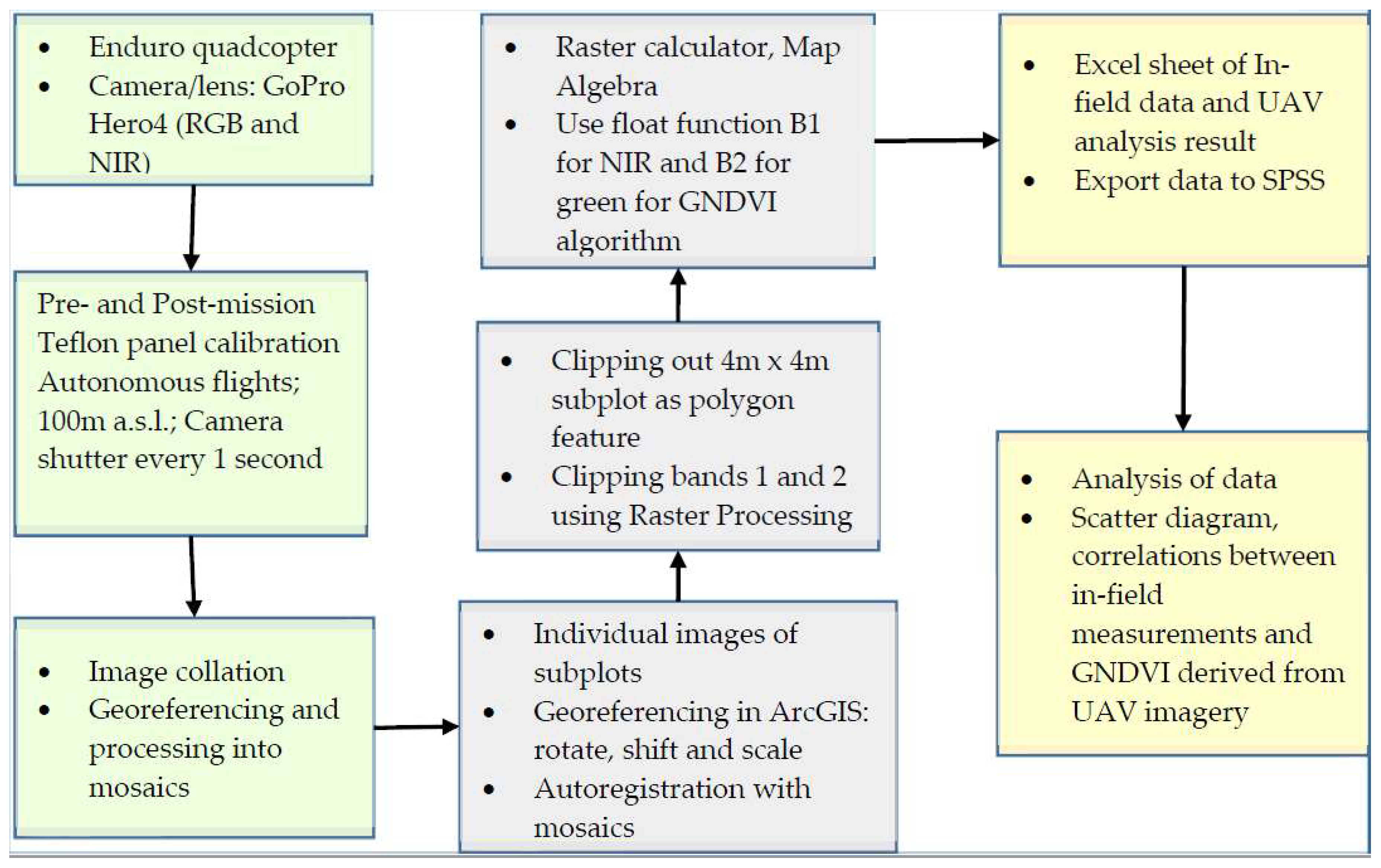
2.4.2. Image Pre-processing and Analysis

In addition to georeferencing and mosaicking of the imageries using Agribotix’s proprietary software, other pre-processing activities needed to be carried out. This included georeferencing of individual images-georeference (GR) of the 4 m × 4 m subplot against the source mosaics (SM) in order to ensure that there is accurate and proportionate representation of space. To achieve this, we adopted two approaches: the automated and manual approaches, using ArcGIS 10.3 (ESRI, Redlands, CA, USA). The automated method worked in majority of the cases but where they did not yield expected results, the manual method was used. For both approaches, the georeferencing tool in ArcGIS is used. Using the fit-to-display, rotate, scale, shift, and auto registration tools to resize, shape, and position, the GR image of each subplot was then brought into the same space as the SM. With regards to the root mean square (RMS) error, an upper limit of 5 was acceptable for those that used the automated method. Most georeferencing using the automated method however had RMS error much lower than 5. Where results of the automated approach do not meet expectations, the manual method was used to link the GR and the SM. Figure 1 below shows a schematic representation of the workflow from field missions through pre-processing, extraction of the GNDVI from UAV imageries to subsequent analysis.

2.4.3. GNDVI from UAV Imagery

Normalized difference vegetation index, the most commonly used vegetation index, first postulated by Rouse [44], quantitatively measures vegetation conditions. It is, essentially, a ratio of the difference and sum of the reflectance in NIR and red bands. However, rather than use the NIR and red bands which are the traditional band combination for NDVI extraction, we use the NIR and green to calculate green normalized difference vegetation index (GNDVI). At lower altitudes, there is no significant scattering of shorter wavelength light and so green performs equally well [41,42]. Thus,

GNDVI = (NIR − G)/(NIR + G),

(1)

where NIR represents reflectance values in the near-infrared band and G represents reflectance values from the green band. The variances in the reflectance properties of the NIR and green bands enable us to assess density and intensity of vegetation using the reflectivity of solar radiation. The utility of a VI such as the NDVI rests on its high correlation with biophysical parameters of plants and low sensitivity to others such that signals from vegetation is enhanced while minimizing solar irradiance and soil background effects [45]. Normalization is achieved by denominating the difference of the NIR and G bands by their sum and by so doing becomes comparable over time and across seasons [46]. Bausch et al. [47] argue that reflectance at green wavelengths is more responsive to variations in leaf chlorophyll and plant health. In concurrence, Burke and Lobell [23] point out that using the green band is more likely to capture differences in nutrient deficiency that are correlated to yields.

Thus, plant vigor is captured by the amount of fluorescence of NIR light in a relatively cheaper sensor with a band order of NIR, green and blue. Thus Equation (1) then transform into

GNDVI = (Band 1 − Band 2)/(Band 1 + Band 2),

(2)

to execute this in ArcMap, the clip function under the data management tool is used to create shapefiles of clipped individual bands of each subplot using the 4 m × 4 m subplot as the output feature. With the raster calculator and using the float functionality in the spatial analyst toolbox, crop vigor is extracted for each subplot using the Algorithm (2). The histogram tab is used to extract relevant statistics: minimum, maximum, mean, and standard deviations for each subplot.

2.5. Data Analysis

In order to demonstrate the reliability of GNDVI derived from UAV imagery for estimating maize crop vigor and yields, linear correlation coefficients were calculated between UAV-derived GNDVI and in-field SPAD meter readings, and yields obtained from the subplots. Both sets of data were to be collected in three parallel rounds in the course of the growing season; about 4–5 weeks after planting (WAP), about 8 WAP, and about 12 WAP. However, due to a combination of logistical and practical as well as weather challenges, the two sets of data collection activities were not always synchronous. For instance, UAV flights routinely require clear and dry skies and so it was quite common to collect in-field data only to find weather conditions unconducive for UAV flights instantaneously. This is particularly true for the second and third rounds of UAV flights. Similarly, practical challenges such as crashes hampered the completion of three rounds of UAV flights for all plots as initially anticipated. In spite of these challenges, we believe enough data points have been generated in order to be able to test our hypothesis.

3. Results

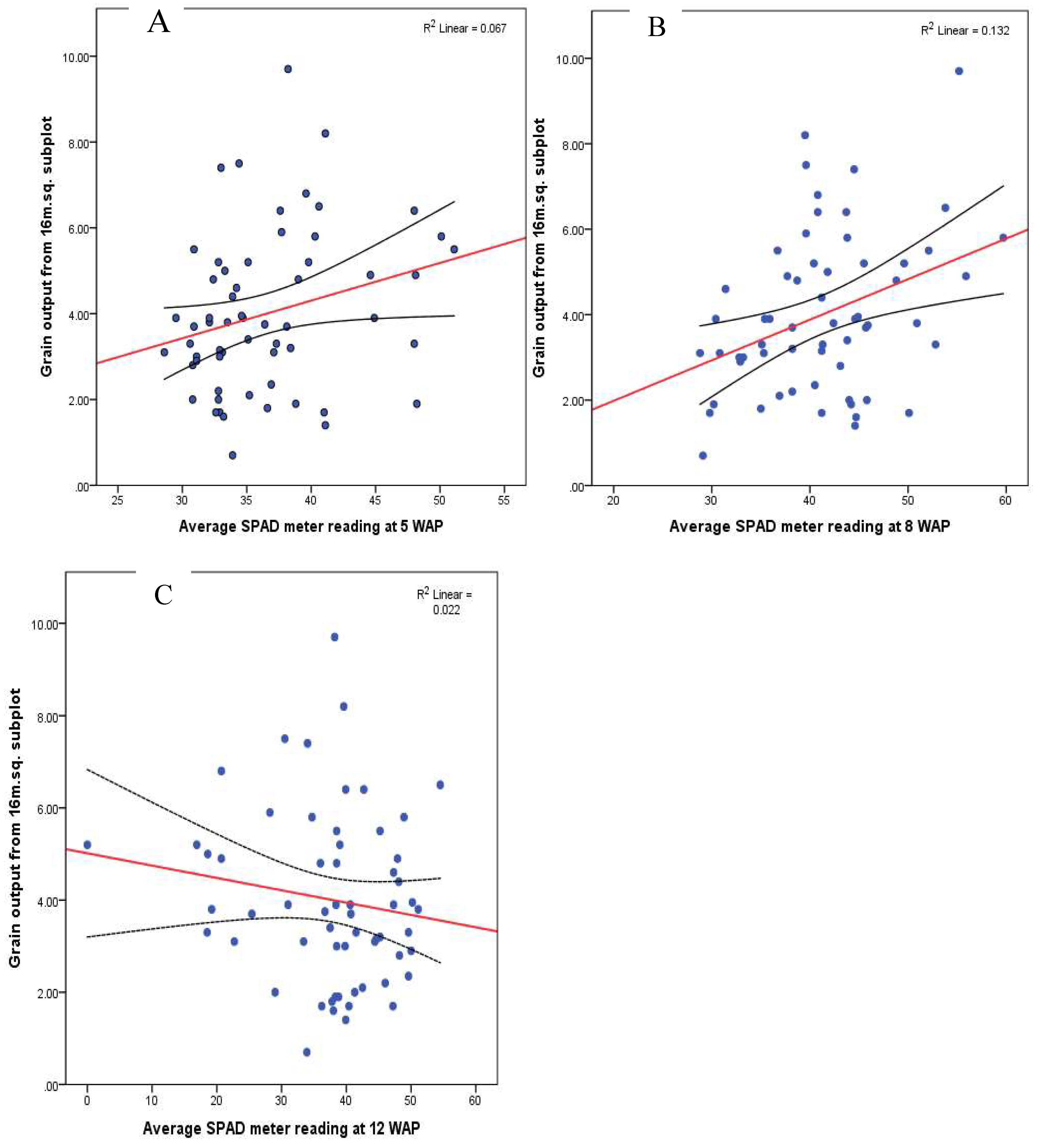
3.1. In-Field Measurements Results

Here, pairwise linear correlations analysis with grain output from the 16 m² subplot—yield—as the dependent variable and crop vigor scores and SPAD meter readings as independent variables are reported. The in-field measurements were carried out at approximately 5, 9, and 13 WAP. Significant positive correlations were obtained for SPAD meter measurements and yields during the vegetative stages of maize development; that is between emergence and about 10 WAP (

Table 1. Correlations between grain output from 16 m² subplot and in-field measurements at 5, 8, and 12 WAP.

SPAD Meter and Yields Correlations
Variables		1	2	3	4
Grain output from 16 m.sq. subplot	Pearson Correlation	1
	Sig. (one-tailed)
	N	60
Average SPAD meter reading at 5 WAP	Pearson Correlation	0.259 *	1
	Sig. (one-tailed)	0.023
	N	60	87
Average SPAD meter reading at 9 WAP	Pearson Correlation	0.363 **	0.205 *	1
	Sig. (one-tailed)	0.002	0.028
	N	60	87	87
Average SPAD meter reading at 13 WAP	Pearson Correlation	−0.150	−0.119	−0.120	1
	Sig. (one-tailed)	0.127	0.137	0.134
	N	60	87	87	87

* Correlation is significant at the 0.05 level (one-tailed); ** Correlation is significant at the 0.01 level (one-tailed).

).

As shown in the Table 1 above, there is a positive and significant; r = 0.259 at 0.05 level; one-tailed correlations between SPAD measurements at 5 WAP and yields; and positive and significant; r = 0.363 at <0.01; one-tailed correlations between SPAD measurements at 9 WAP and yields. These modest relations however fade by the 13th WAP when maize crops tasseled and silked and are in senescence. At these latter stages of the crop growth cycle, correlations between SPAD measurements and yields from the subplot become negative and non-significant. These relationships are shown in Figure 2A–C below:

It is also pertinent to note that as modest as these correlation results are, they are relatively better at estimating final yields compared to visually estimating maize crop vigor. As

Table 2. Correlations between grain output from 16 m² subplot and maize vigor score for 5, 9, and 13 WAP

Bivariate Correlation Analyses between In-Field Measures
Variables		1	2	3	4
Grain output from 16 m.sq. subplot	Pearson Correlation	1
	Sig. (one-tailed)
	N	60
Crop vigor score at 5 WAP	Pearson Correlation	−0.140	1
	Sig. (one-tailed)	0.142
	N	60	87
Crop vigor score at 9 WAP	Pearson Correlation	0.122	0.673 **	1
	Sig. (one-tailed)	0.177	0.000
	N	60	87	87
Crop vigor score at 13 WAP	Pearson Correlation	0.226 *	0.444 **	0.516 **	1
	Sig. (one-tailed)	0.041	0.000	0.000
	N	60	87	87	87

* p < 0.05; ** p < 0.01.

below shows, the correlations are only significant r = 0.226 at p = 0.05; one-tailed at around 13 WAP. Indeed, there are no significant relationship between visual scores of maize vigor and final output at 5 WAP and 8 WAP.

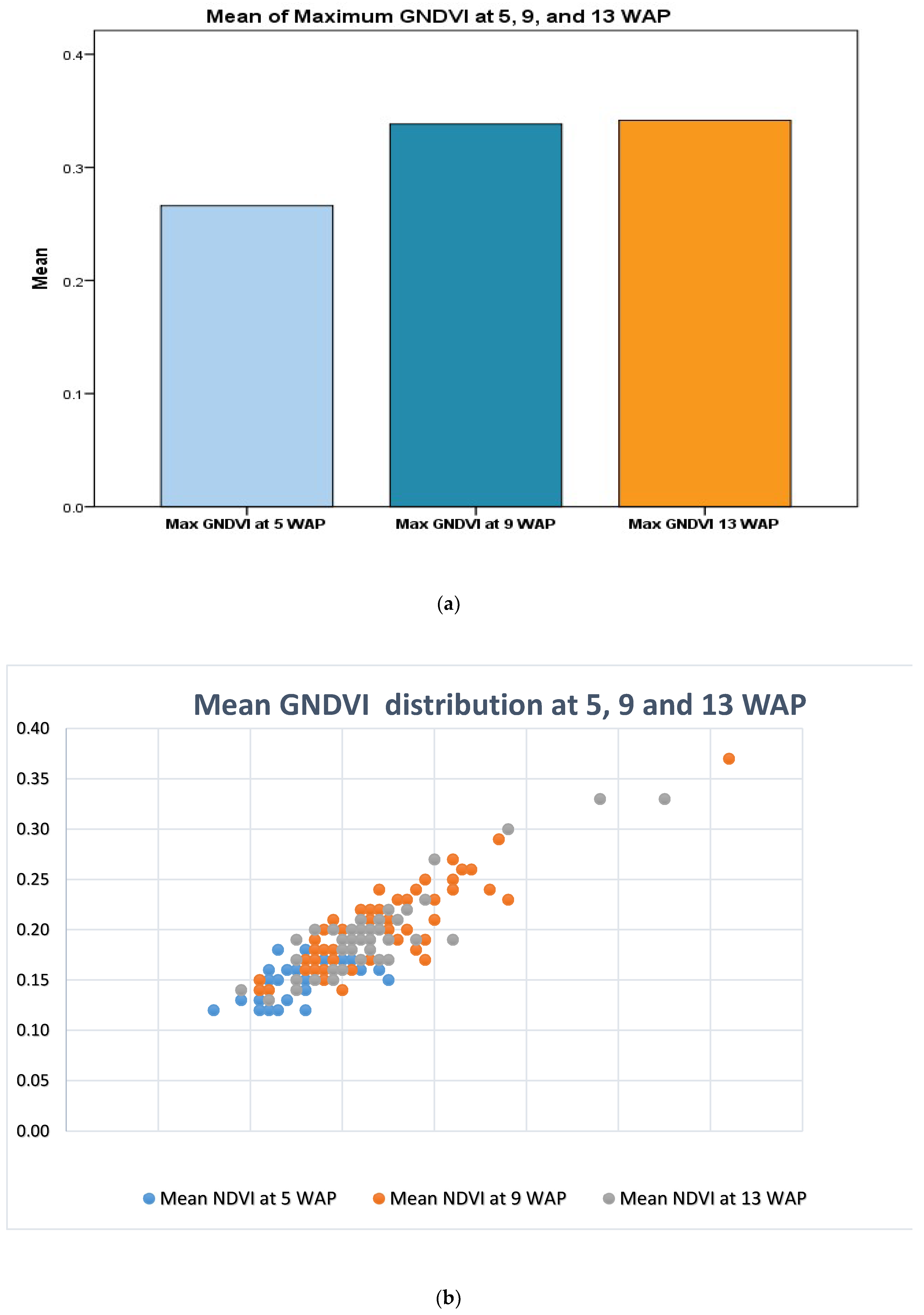
3.2. UAV GNDVI Results

For starters, summary descriptive statistics for the maximum and mean GNDVI are extracted from the UAV images captured at about 5, 9, and 13 WAP and presented here. As

Table 3. Descriptive statistics of maximum and mean GNDVI at 5, 8, and 12 WAP

Descriptive Statistics
	N	Range	Minimum	Maximum	Mean	Std. Deviation
Max GNDVI at 5 WAP	58	0.19	0.16	0.35	0.2609	0.03845
Max GNDVI at 9 WAP	74	0.51	0.21	0.72	0.3354	0.07406
Max GNDVI 13 WAP	44	0.46	0.19	0.65	0.3302	0.08236
Mean GNDVI at 5 WAP	58	0.09	0.12	0.21	0.1541	0.02009
Mean GNDVI at 9 WAP	74	0.24	0.13	0.37	0.2014	0.03801
Mean GNDVI 13 WAP	44	0.20	0.13	0.33	0.1950	0.04332
Valid N (listwise)	18

below shows, the maximum GNDVI for 5 WAP is 0.35 which then increases to a zenith of 0.72 at around 9 WAP before slightly decreasing to 0.65 by the 13 WAP.

The mean GNDVI also exhibits similar trends which implies that maize crop NDVI peaks around 9 WAP-0.37 and 0.20 for maximum and mean, respectively (Table 3). This is graphically displayed where the average of the maximum GNDVI increases from 0.26 at 5 WAP to 0.33 at 9 WAP (Figure 3A). However, not much differences are discernible between the distribution of maximum GNDVI at 9 and 13 WAP (Figure 3B).

More to the point, pairwise linear correlation analysis showed a strong association between higher maximum and mean GNDVI extracted from subplots and the grain yields from those subplots. For example, at 5 WAP, correlations between maximum GNDVI and yields is positive and significant; r = 0.393, at p < 0.01 level while that between mean GNDVI and yields was similarly positive and significant; r = 0.372, at p < 0.01 (

Table 4. Bivariate analysis between output from subplot and UAV-derived GNDVI at 5, 9, and 13 WAP

Bivariate Correlation Analysis between Yields and UAV-Derived GNDVI Measures
Variables		1	2	3	4	5	6	7
Grain output from 16 m.sq. subplot	Pearson Correlation	1
	Sig. (one-tailed)
	N	60
Max GNDVI at 5 WAP	Pearson Correlation	0.393 **	1
	Sig. (one-tailed)	0.006
	N	41	58
Max GNDVI at 9 WAP	Pearson Correlation	0.131	0.342 **	1
	Sig. (one-tailed)	0.182	0.006
	N	50	53	74
Max GNDVI 13 WAP	Pearson Correlation	0.123	0.359 *	0.046	1
	Sig. (one-tailed)	0.267	0.046	0.390
	N	28	23	39	44
Mean GNDVI at 5 WAP	Pearson Correlation	0.372 **	0.645 **	0.584 **	0.369 *	1
	Sig. (one-tailed)	0.008	0.000	0.000	0.042
	N	41	58	53	23	58
Mean GNDVI at 9 WAP	Pearson Correlation	0.041	0.393 **	0.865 **	−0.033	0.545 **	1
	Sig. (one-tailed)	0.389	0.002	0.000	0.421	0.000
	N	50	53	74	39	53	74
Mean GNDVI 13 WAP	Pearson Correlation	0.156	0.411 *	0.076	0.893 **	0.401 *	0.010	1
	Sig. (one-tailed)	0.213	0.026	0.323	0.000	0.029	0.476
	N	28	23	39	44	23	39	44

Notes: ** p < 0.05; * p < 0.01.

). This implies that GNDVI derived from UAV imagery is relatively a better, albeit, weak predictor of maize yields compared to in-field measures such as SPAD meter readings which also returned positive and significant correlations; r = 0.259, p = 0.023 at around the same stages of the crop development.

These relationships between mean and maximum GNDVI at 5 WAP however wane by 9 WAP and 13 WAP (Table 4). At these latter stages, there are no associations between GNDVI measures and yields. Compared to in-field measures using the SPAD meter readings—r = 0.363, p < 0.01—at 9 WAP, and visual scoring of crop vigor—r = 0.226, p = 0.041—at 13 WAP, GNDVI measures fare poorly with regards to the latter stages of the crop development.

4. Discussion

This study was aimed at demonstrating the reliability of GNDVI derived from a UAV platform for estimating maize crop vigor and yields on complex smallholder farms. Our results demonstrate that GNDVI extracted from modified consumer-grade cameras mounted on UAVs can be used to accurately predict not just maize crop vigor but also yields. The strongest relationship between mean and maximum GNDVI at 5 WAP is consistent with the findings of Raun et al. [48] on wheat, Shanahan et al. [32] on maize and Swain et al. [31] on rice at similar stages. Most crucially, our results show that GNDVI exhibits the strongest relationship with yields—r = 0.372 and r = 0.393 for mean and maximum GNDVI respectively at 5 WAP. This is followed by SPAD meter readings with yields—r = 0.259 and r = 0.363 at 5 WAP and 9 WAP respectively. Finally, visual score also returned significant relations—r = 0.226 but only at 13 WAP. Our results showing UAV-based measures performing better relative to ground-based ones such as SPAD measurements was expected given that while the latter takes into consideration only a sample of the crops on the subplot, the former captures the entirety of the crops in the subplot. That is, UAV-based measures would be more comprehensive and a better measure of crop health compared to ground-based measures such as SPAD readings and visual scores.

The point of departure with other studies however is the results we obtained around the middle of the growing season. As Table 4 shows, the relationship between yields and GNDVI at 5 WAP disappear by 9 WAP. This is contrary to the results obtained by Teal et al. [49] who found the strengthening of the relationship at similar stages before disappearing in maize senescence. Our finding of the non-significance of the relationship could be attributed to a number of confounding factors. One such factor is moisture stress, particularly for rainfed maize crops. Severe water stress at critical growth stages would not only lead to canopy closure and so obstruct the sensor’s field of view but, more crucially, affect the productivity of the crops. Another important potential confounding factor for the non-significance of the relationship between yields and GNDVI at 9 WAP is the likely varying farm management practices such as weed control and cropping systems. With regards to cropping systems for example, plots intercropped with cassava, beans, cocoyams, among others could have their mean and maximum GNDVI measures artificially increased compared to monocropped plots. Similarly, plots with poorly controlled weeds may anecdotally have artificially high NDVI metrics and lower yields which would be counterintuitive to the hypothesis of this study which is that plots with higher mean and maximum GNDVI would have higher yields.

The results also demonstrate that the UAV system and the methods used to extract NDVI metrics could be used to produce yield maps for entire plots. Such yield maps would show spatial variations in yields and provide spatial information of not only crop vigor but yields, even in such complex farming systems like the settings of this study [23]. The major advantage that such a yield map would have over in-field methods for ascertaining crop status in the course of the growing season is that it offers a bird’s eye view of the plot and so could serve as a decision support system as is currently being trialed in parts of Mozambique [50]. Here, farm intelligence gleaned from a UAV system is being used by smallholder farmers, through extension workers, to make informed decisions on beans, rice, and maize cultivation. This has the potential to significantly improve crop yield levels and contribute to improving yield levels on SSA farms.

In terms of future research directions, similar experiments could be carried out but under more controlled conditions so that there would be controls for differing farm management activities such as mono- and inter-cropped plots as well as for differing weed management regimes. Such controls could demonstrate the actual potential of a UAV platform for applications in agriculture. What our study shows is the potential of this system in spite of the numerous obfuscations emanating from the rainfed and complex nature of smallholder farming systems in SSA. Already, Burke and Lobell [23] have demonstrated the potential of achieving accurate predictions of yields on small farms in Western Kenya using the one-meter spatial resolution Terra Bella satellite data. Another area for future research is the application of our methodology to rice (Oryza sativa, L.); a much more apt crop for two reasons. First, unlike maize, rice is usually mono-cropped and cultivated on relatively larger farm sizes. Thus, most of the limitations enumerated with regards to intercrops might not inhere. Second, rice fields are often flooded and become inaccessible. It is during periods when fields are physically difficult to traverse that the RS approach as used here could be most useful in ascertaining not just the vigor of the crops but also the intra-field variability.

An important limitation of the present study is the failure to normalize the individual VIS bands prior to calculating the vegetation index. While normalization is often recommended in the literature [20,51] such that γ = G /(R + G + B), where γ is the normalized green band, we did not find the need for this in the present study. Most studies which applied normalization as above such as Ballesteros et al. [52] and Saberioon et al. [51] relied on a normal RGB camera while we employed a modified lens in which the R channel had been replaced with the NIR channel. Indeed, in the case of Saberioon et al. [51] the stated aim of their study was to use all the VIS bands derived from images captured and thus normalization was unavoidable. This notwithstanding, a future study should explore the possibility of normalization of the bands, even for a modified camera, as this could further improve the results we obtained for the present study.

5. Conclusions

Overall, our results demonstrate that GNDVI derived from UAV is not only useful in ascertaining maize crop vigor and but also estimating yields and that it indeed performs comparatively better when compared to in-field methods of SPAD meter measurement and visual scoring of crop vigor. Thus, UAV-derived GNDVI is a better, most timeous, more efficient, and objective measure of crop vigor and predictor of maize yields compared to in-field methods. The GNDVI method as used here is also the most desired if the objective is to provide decision support for smallholder farmers given that it gives these results at the earliest—5 WAP; compared to SPAD measurements—9 WAP; and visual scoring—13 WAP. It thus could afford farmers the opportunity to take remedial actions to improve final yields by targeting critical farm management activities such as fertilizer application and irrigation rather than treat whole plots as homogeneous units.

The relatively poor performance at 5 WAP and even 9 WAP of the visual scoring approach to assessing crop health and thus expectations with regards to yields by close of the farming season implies that it is not an approach that can be relied on by farmers to take farm decisions. Its relatively improved performance close to the season’s end eliminates its utility as not much could be done to remedy a poor season. The relatively better performance of the UAV-derived GNDVI as early as 5 WAP is the highlight of this study and bodes well for improving yields even on complex smallholder farms in SSA.

References

1. FAOSTAT. Food and Agriculture Organization’s Statistical Database. FAO, 2017. Available online: http://www.Fao.Org/faostat/en/#home (accessed on 21 February 2017).
2. Dzanku, F.M.; Jirström, M.; Marstorp, H. Yield gap-based poverty gaps in rural Sub-Saharan Africa. World Dev. 2015, 67, 336–362. [Google Scholar] [CrossRef]
3. Swain, K.C.; Zaman, Q.U. Rice crop monitoring with unmanned helicopter remote sensing images. In Remote Sensing of Biomass—Principles and Applications; Fatoyinbo, L., Ed.; INTECH Open Access Publisher: Rijeka, Croatia, 2012; pp. 253–272. [Google Scholar]
4. Srbinovska, M.; Gavrovski, C.; Dimcev, V.; Krkoleva, A.; Borozan, V. Environmental parameters monitoring in precision agriculture using wireless sensor netweorks. J. Clean. Prod. 2015, 88, 297–307. [Google Scholar] [CrossRef]
5. Jones, H.G.; Vaughan, R.A. Remote Sensing of Vegetation: Principles, Techniques, and Applications, 1st ed.; Oxford University Press: Oxford, UK, 2010. [Google Scholar]
6. Benincasa, P.; Antognelli, S.; Brunetti, L.; Fabbri, C.A.; Natale, A.; Sartoretti, V.; Modeo, G.; Guiducci, M.; Tei, F.; Vizzari, M. Reliability of NDVI derived by high resolution satellite and UAV compared to in-field methods for the evaluation of early crop n status and grain yield in wheat. Exp. Agric. 2017, 54, 604–622. [Google Scholar] [CrossRef]
7. Fageria, N.K. Nitrogen harvest index and its association with crop yields. J. Plant Nutr. 2014, 37, 795–810. [Google Scholar] [CrossRef]
8. Chapman, S.C.; Merz, T.; Chan, A.; Jackway, P.; Hrabar, S.; Dreccer, M.F.; Holland, E.; Zheng, B.; Ling, T.J.; Jimenez-Berni, J. Pheno-copter: A low-altitude, autonomous remote sensing robotic helicopter for high-throughput field-based phenotyping. Agron. J. 2014, 4, 279–301. [Google Scholar] [CrossRef]
9. Lobell, D.B. The use of satellite data for crop yield gap analysis. Field Crops Res. 2013, 143, 56–64. [Google Scholar] [CrossRef]
10. Bisht, P.; Kumar, P.; Yadav, M.; Rawat, J.S.; Sharma, M.P.; Hooda, R.S. Spatial dynamics for relative contribution of cropping pattern analysis on environment by integrating remote sensing and GIS. Int. J. Plant Prod. 2014, 8, 1735–8043. [Google Scholar]
11. Jovanović, D.; Govedarica, M.; Rašić, D. Remote sensing as a trend in agriculture. Res. J. Agric. Sci. 2014, 46, 32–37. [Google Scholar]
12. Roumenina, E.; Atzberger, C.; Vassilev, V.; Dimitrov, P.; Kamenova, I.; Banov, M.; Filchev, L.; Jelev, G. Single- and multi-data crop identification using PROBA-V 100 and 300 m S1 products on Zlatia test site, Bulgaria. Remote Sens. 2015, 7, 13843–13862. [Google Scholar] [CrossRef]
13. Pinter, P.J.J.; Hatfield, J.L.; Schepers, J.S.; Barnes, E.M.; Moran, M.S.; Daughtry, C.S.T.; Upchurch, D.R. Remote sensing for crop management. Photogramm. Eng. Remote Sens. 2003, 69, 647–664. [Google Scholar] [CrossRef]
14. Yao, X.; Huang, Y.; Shang, G.; Zhou, C.; Cheng, T.; Tian, Y.; Cao, W.; Zhu, Y. Evaluation of six algorithms to monitor wheat leaf nitrogen concentration. Remote Sens. 2015, 7, 14939–14966. [Google Scholar] [CrossRef]
15. Frazier, A.E.; Wang, L.; Chen, J. Two new hyperspectral indices for comparing vegetation chlorophyll content. Geo-Spat. Inf. Sci. 2014, 17, 17–25. [Google Scholar] [CrossRef] [Green Version]
16. Liang, L.; Qin, Z.; Zhao, S.; Di, L.; Zhang, C.; Deng, M.; Lin, H.; Zhang, L.; Wang, L.; Liu, Z. Estimating crop chlorophyll content with hyperspectral vegetation indices and the hybrid inversion method. Int. J. Remote Sens. 2016, 37, 2923–2949. [Google Scholar] [CrossRef]
17. Imran, M.; Stein, A.; Zurita-Milla, R. Using geographically weighted regression kriging for crop yield mapping in West Africa. Int. J. Geogr. Inf. Sci. 2015, 29, 234–257. [Google Scholar] [CrossRef]
18. Jaafar, H.H.; Ahmad, F.A. Crop yield prediction from remotely sensed vegetation indices and primary productivity in arid and semi-arid lands. Int. J. Remote Sens. 2015, 36, 4570–4589. [Google Scholar] [CrossRef]
19. Cheng, T.; Yang, Z.; Inoue, Y.; Zhu, Y.; Cao, W. Recent advances in remote sensing for crop growth monitoring. Remote Sens. 2016, 8, 116. [Google Scholar] [CrossRef]
20. Torres-Sánchez, J.; Peña, J.M.; de Castro, A.I.; López-Granados, F. Multi-temporal mapping of the vegetation fraction in early-season wheat fields using images from UAV. Comput. Electron. Agric. 2014, 103, 104–113. [Google Scholar] [CrossRef] [Green Version]
21. Wójtowicz, M.; Wójtowicz, A.; Piekarczyk, J. Application of remote sensing methods in agriculture. Commun. Biometry Crop Sci. 2016, 11, 31–50. [Google Scholar]
22. Berni, J.A.; Zarco-Tejada, P.J.; Suárez, L.; Fereres, E. Thermal and narrowband multispectral remote sensing for vegetation monitoring from an unmanned aerial vehicle. IEEE Trans. Geosci. Remote Sens. 2009, 47, 722–738. [Google Scholar] [CrossRef] [Green Version]
23. Burke, M.; Lobell, D.B. Satellite-based assessment of yield variation and its determinants in smallholder African systems. Proc. Natl. Acad. Sci. USA 2017, 114, 2189–2194. [Google Scholar] [CrossRef] [PubMed] [Green Version]
24. Yang, C.; Hoffmann, W.C. Low-cost single-camera imaging system for aerial applicators. J. Appl. Remote Sens. 2015, 9, 096064. [Google Scholar] [CrossRef] [Green Version]
25. Matese, A.; Toscano, P.; Gennaro, S.F.; Genesio, L.; Vaccari, F.P.; Primicerio, J.; Belli, C.; Zaldei, A.; Bianconi, R.; Gioli, B. Intercomparison of UAV, aircraft and satellite remote sensing platforms for precision viticulture. Remote Sens. 2015, 7, 2971–2990. [Google Scholar] [CrossRef]
26. Colwell, R.N. Determining the prevalence of certain cereal crop diseases by means of aerial photography. Hilgardia 1956, 26, 223–286. [Google Scholar] [CrossRef] [Green Version]
27. Laliberte, A.S.; Goforth, M.A.; Steele, C.M.; Rango, A. Multispectral remote sensing from unmanned aircraft: Image processing workflows and applications for rangeland environments. Remote Sens. 2011, 3, 2529–2551. [Google Scholar] [CrossRef]
28. Sakamoto, T.; Gitelson, A.A.; Nguy-Robertson, A.L.; Arkebauer, T.J.; Wardlow, B.D.; Suyker, A.E.; Verma, S.B.; Shibayama, M. An alternative method using digital cameras for continuous monitoring of crop status. Agric. For. Meteorol. 2013, 154–155, 113–126. [Google Scholar] [CrossRef]
29. Piekarczyk, J.; Sulewska, H.; Szymańska, G. Winter oilseed-rape yield estimates from hyperspectral radiometer measurements. Quaest. Geogr. 2011, 30, 77–84. [Google Scholar] [CrossRef]
30. Zhang, J.; Yang, C.; Song, H.; Hoffmann, W.S.; Zhang, D.; Zhang, G. Evaluation of an airborne remote sensing platform consisting of two consumer-grade cameras for crop identification. Remote Sens. 2016, 8, 257. [Google Scholar] [CrossRef]
31. Swain, K.C.; Thomson, S.J.; Jayasuriya, H.P.W. Adoption of an unmanned helicopter for low-altitude remote sensing to estimate yield and total biomass of a rice crop. Am. Soc. Agric. Biol. Eng. 2010, 53, 21–27. [Google Scholar]
32. Shanahan, J.F.; Schepers, J.S.; Francis, D.D.; Varvel, G.E.; Wilhelm, W.W.; Tringe, J.M.; Schlemmer, M.R.; Major, D.J. Use of remote sensing imagery to estimate corn grain yield. Agron. J. 2001, 93, 583–589. [Google Scholar] [CrossRef]
33. GSS. 2010 Population and Housing Census: District Analytical Report. Upper Manya Krobo District; Ghana Statistical Service, Ed.; Ghana Statistical Service: Accra, Ghana, 2014. [Google Scholar]
34. GSS. 2010 Population and Housing Census: District Analytical Report. Lower Manya Krobo Municipality; Ghana Statistical Service, Ed.; Ghana Statistical Service: Accra, Ghana, 2014. [Google Scholar]
35. Djurfeldt, G.; Aryeetey, E.; Isinika, A.C.E. African Smallholders: Food Crops, Markets and Policy; Djurfeldt, G., Aryeetey, E., Isinika, A.C., Eds.; CAB International: Oxfordshire, UK, 2011; 397p. [Google Scholar]
36. Wood, C.W.; Reeves, D.W.; Himelrick, D.G. (Eds.) Relationships between Chlorophyll Meter Readings and Leaf Chlorophyll Concentration, N Status, and Crop Yield: A Review; Agronomy Society of New Zealand: Palmerston North, New Zealand, 1993; Volume 23. [Google Scholar]
37. FAO. Guidelines for Soil Description; Food and Agriculture Organization of the United Nations: Rome, Italy, 2006. [Google Scholar]
38. Carletto, C.; Jolliffe, D.; Banerjee, R. From trajedy to renaissance: Improving agricultural data for better policies. J. Dev. Stud. 2015, 51, 133–148. [Google Scholar] [CrossRef]
39. Sud, U.C.; Ahmad, T.; Gupta, V.K.; Chandra, H.; Sahoo, P.M.; Aditya, K.; Singh, M.; Biswas, A. Methodology for Estimation of Crop Area and Crop Yield under Mixed and Continuous Cropping; ICAR-Indian Agricultural Statistics Research Institute: New Delhi, India, 2017. [Google Scholar]
40. Underhill, J. Personal communication through email to first author on 31 May 2018, 2018.
41. Agribotix. Colorado: Agribotix. 2018. Available online: https://agribotix.com/blog/2017/04/30/comparing-rgb-based-vegetation-indices-with-ndvi-for-agricultural-drone-imagery/ (accessed on 4 June 2018).
42. Agribotix. How do You do NDVI? Agribotix: Boulder, CA, USA, 2013. Available online: https://agribotix.com/farm-lens-faq/ (accessed on 3 June 2018).
43. Mesas-Carrascosa, F.-J.; Torres-Sánchez, J.; Clavero-Rumbao, I.; García-Ferrer, A.; Peña, J.-M.; Borra-Serrano, I.; López-Granados, F. Assessing optimal flight parameters for generating accurate multispectral Orthomosaicks by UAV to support site-specific crop management. Remote Sens. 2015, 7, 12793–12814. [Google Scholar] [CrossRef]
44. Rouse, J.W.; Haas, R.H.; Schell, J.A.; Deering, D.W. (Eds.) Monitoring Vegetation Systems in the Great Plains with ERTS; Third ERTS Symposium, December 1973; The National Aeronautics and Space Administration Goddard Space Flight Centre: Greenbelt, MD, USA, 1973. [Google Scholar]
45. Jackson, R.D.; Huete, A.R. Interpreting vegetation indices. Prev. Vet. Med. 1991, 11, 185–200. [Google Scholar] [CrossRef]
46. Tucker, C.J. Red and photographic infrared linear combinations for monitoring vegetation. Remote Sens. Environ. 1978, 8, 127–150. [Google Scholar] [CrossRef]
47. Bausch, W.C.; Halvorson, A.D.; Cipra, J. Quickbird satellite and ground-based multispectral data correlations with agronomic parameters of irrigated maize grown in small plots. Biosyst. Eng. 2008, 101, 306–315. [Google Scholar] [CrossRef]
48. Raun, W.R.; Johnson, G.V.; Stone, M.L.; Sollie, J.B.; Lukina, E.V.; Thomason, W.E.; Schepers, J.S. In-season prediction of potential grain yield in winter wheat using canopy reflectance. Agron. J. 2001, 93, 131–138. [Google Scholar] [CrossRef]
49. Teal, R.K.; Tubana, B.; Girma, K.; Freeman, K.W.; Arnall, D.B.; Walsh, O.; Raun, W.R. In-season prediction of corn grain yield potential using normalized difference vegetation index. Agron. J. 2006, 98, 1488–1494. [Google Scholar] [CrossRef]
50. AU. Drones on the Horizon: Transforming Africa’s Agriculture; The African Union-The New Partnership for Africa’s Development: Gauteng, South Africa, 2018. [Google Scholar]
51. Saberioon, M.M.; Amin, M.S.M.; Anuar, A.R.; Gholizadeh, A.; Wayayok, A.; Khairunniza-Bejo, S. Assessment of rice leaf chlorophyll content using visible bands at different growth stages at both the leaf and canopy scale. Int. J. Appl. Earth Obs. Geoinf. 2014, 32, 35–45. [Google Scholar] [CrossRef]
52. Ballesteros, R.; Ortega, J.F.; Hernandez, D.; del Campo, A.; Moreno, M.A. Combined use of agro-climatic and very high-resolution remote sensing information for crop monitoring. Int. J. Appl. Earth Obs. Geoinf. 2018, 72, 66–75. [Google Scholar] [CrossRef]
Figure 1. UAV image analysis workflow showing field data collection (left), GNDVI extraction (center), and data analysis (right).
Drones 02 00028 g001
Figure 2. Scatterplot of the correlations between grain output from subplot and SPAD meter measurements of crop vigor at 5 (A), 9 (B), and 13 (C) WAP.
Drones 02 00028 g002
Figure 3. (a) Simple bar chart of average maximum GNDVI at 5, 9, and 13 WAP; (b) Scatter distribution of mean GNDVI at 5, 9, and 13 WAP.
Drones 02 00028 g003